Calibration Method for Line-Structured Light Three-Dimensional Measurement Based on a Simple Target

Abstract

Line-structured light three-dimensional (3D) measurement is apt for measuring the 3D profile of objects in complex industrial environments. The light-plane calibration, which is a crucial link, greatly affects the accuracy of measurement results. This paper proposes a novel calibration method for line-structured light 3D measurement based on a simple target, i.e., a single cylindrical target (SCT). First, the line-structured light intersects with the target to generate a light stripe. Meanwhile, the camera captures the calibration images, extracts the refined subpixel center points of the light stripe (RSCP) and detects the elliptic profiles of the two ends of the cylindrical target (EPCT). Second, two elliptical cones defined by the EPCT and the camera optical center are determined. Combining the two defined elliptical cones and the known radius of the SCT, we can uniquely solve the axis equation of the SCT. Finally, because the coordinates of RSCP in the camera coordinate system fulfill both the camera model and the cylindrical equation, these coordinates can be solved and used to obtain the optimal solution of the light-plane equation. The results of simulations and experiments verify that our proposed method has higher accuracy and effectiveness.

1. Introduction

Three-dimensional (3D) measurements are widely performed in industrial automation quality verification, industrial reverse design, surface-deformation tracking, and 3D reconstruction for object recognition [1,2,3]. Commonly, 3D measurement methods can be divided into two categories, namely contact measurements and noncontact measurements. With the rapid development of industrial production, noncontact measurement is more important, especially vision measurement. Among the many vision-measurement methods, the light-structured vision-measurement method plays an important role in some industrial environments, such as online pipeline product inspection, noncontact reverse engineering, and computer animation, because of its advantages of being noncontact, nondestructive, rapid, full-field, and high-precision [4,5,6]. According to the type of projected light, there are three categories of light-structured vision-measurement method: the point-structured light method, line-structured light method, and coded-structured light method. The point-structured light method can obtain one-dimensional data, i.e., a single measurement can obtain the distance of a point, which is commonly suitable for range measurement. If 3D measurement based on the point-structured light method is required, a precision mechanical motion is essential (e.g., Leica 3D DISTO). The coded-structured light method [7,8,9] adopts a projector to cast the coding patterns, and meanwhile, a camera captures the patterns distorted by the surface of the object. Because of the limited power of the projector, the coded-structured light method is not suitable for complex industrial environments, especially metallic surfaces. In recent years, with the rise of intelligent driving and industry, laser-scanning-measurement technology (e.g., laser-scanning measurement with galvanometer scanners) [10,11] has developed greatly, which is to measure the one- or two-dimensional information by the precise movement of a laser beam. The technology is suitable for large scene measurement, as well as for desktop precise measurement. However, this technology usually requires precision mechanical structures, which brings harsh manufacturing difficulty and tedious training procedures. The line-structured light method involves the use of a large-power line laser and a camera to construct a 3D optical sensor. The line-structured light method aided by laser triangulation can measure the 3D profile of the object in complex industrial environments, such as weld-quality inspection, chip-pin detection, and printed circuit-board (PCB)-quality inspection. Moreover, the line-structured light method also has the advantages of simplicity, high precision, and high measurement speed [12].

In the line-structured light method, the essence is how to convert the two-dimensional (2D) light-stripe information into 3D-coordinate information. This means that the system calibration, which is a crucial link, greatly affects the accuracy of the measurement results. The system calibration consists of the camera calibration and the light-plane calibration. Among them, the camera calibration is mainly to obtain the intrinsic parameters of the camera, and many related studies have been published in the past [13,14,15,16,17]. In our research, we assume that the camera has been calibrated, i.e., the intrinsic parameters of rhe camera are known. Thus, the focus of this paper is the calibration of light-plane parameters. Depending on the form of the calibration target, the one-dimensional (1D)-, 2D-, and 3D-target light-plane methods are widely reported [18,19,20,21,22,23,24,25,26,27]. For the 1D-target method, Wei, et al. [18] proposed a calibration method based on a 1D target. The series of intersecting points between the light plane and the 1D target were determined using the known distance between the characteristic points of the 1D target. Liu et al. [19] reported a calibration method using a free-moving 1D target. The intersections between the free-moving 1D target and the light plane were solved according to the cross-ratio invariance, and the light plane was fitted using the obtained intersections. For the 2D-target method, Zhou et al. [20] proposed an on-site calibration method based on a planar target, and the calibration points were obtained through repeated target movements. Zhang et al. [21] also reported a higher-precision calibration method using a planar target, where the line of light stripes was described utilizing the Plück matrix. The existing 1D and 2D targets are easy to manufacture and simple to maintain, but the methods based on the 1D and 2D target cannot be calibrated to depend only on one image. For the 3D-target method, the 3D-constraint relationship of calibration can utilize the 3D target itself. Some researchers [22,23,24] introduced a 3D target to determine the light-plane calibration points based on the cross-ratio invariability, but these kinds of methods were complex and low-precision. Liu et al. [25] developed a calibration method using a single-ball target. The method is based on the fact that the profile of the ball target is unaffected by its position and posture of the ball target. Liu et al. [26] also proposed a calibration method based on a parallel cylindrical target. The line-structured light intersects the parallel cylindrical target to solve a minor axis of the auxiliary cone, thereby obtaining the light-plane Equation. Liu’s two methods have the simple calibration process and the 3D-constraint stability in a complex environment. However, neither the standard ball target nor the parallel cylindrical target are easy to manufacture. Zhu et al. [27] proposed a calibration method based on an SCT. The calibration target used in the method is a cylinder, which is very simple. However, the method took advantage of the symmetry of the cylinder, that is, the position and posture of the target have special requirements.

In this paper, we present a novel calibration method for line-structured light 3D measurement through utilizing a simple target, i.e., a single cylindrical target (SCT). The main reasons for selecting a cylinder as the calibration object are its ease of manufacture and low cost. Compared with the method using a SCT reported in literature [27], the position and posture of the calibration target in our study is free. Firstly, the line-structured light 3D-measurement model is established. Secondly, the principle of the light-plane calibration with a SCT is presented, and the main contents include the following: (1) the refined subpixel centerpoints (RSCP) are extracted by the introduced Steger’s method and the elliptic profiles of the two ends of the cylindrical target (EPCT) are detected with the introduced “revisited arc-support line segment (RALS) method”. (2) The two elliptical cones defined by the two end circles of the SCT and the camera optical center are determined. Combining the two defined elliptical cones and the known radius of the SCT, we can uniquely solve the axis equation of the SCT. (3) The coordinates of the RSCP in the camera coordinate system should satisfy two conditions: the camera model and the cylindrical equation. Then, the light-plane equation is calculated by utilizing nonlinear optimization. Finally, the accuracy and effectiveness of our proposed method are verified through simulations and experiments.

The paper is organized as follows: Section 2 presents the line-structured light 3D-measurement model. Section 3 outlines the principle of the light-plane calibration based on the SCT. Section 4 and Section 5 describe simulations and experiments. Section 6 concludes the study. Finally, in the Appendix A, we derive two geometry conclusions used in this paper.

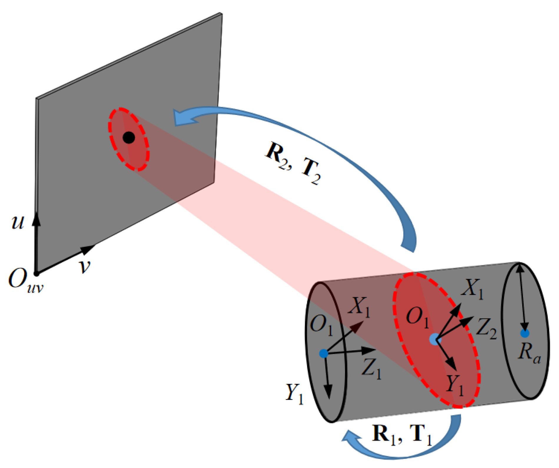
2. Line-Structured Light 3D-Measurement Model

Figure 1 shows the schematic diagram of the model for the line-structured light 3D-measurement with an SCT. A line laser is cast onto the SCT by the laser projector, after which the camera captures the light-stripe images distorted by the cylinder surface. Finally, the 3D coordinates of the points on the light stripe are determined. In Figure 1, O_c(O_w) is the optical center. (O_w; X_w, Y_w, Z_w) and (O_c; X_c, Y_c, Z_c) represent the world coordinate system (WCS) and the camera coordinate system (CCS), respectively. Here, for the simplicity of analysis, WCS and CCS are set to identical. In the CCS, there is an arbitrary point, p_c, on the intersection of the light plane and the surface of the measured object. p_c is projected onto the normalized image plane to generate p_n. The lens distortion of the camera will affect p_n, especially in the radial direction, which causes the shift from p_n to p_d. Therefore, the camera model can be expressed as

$$\left(\begin{array}{c}u\\ v\\ 1\end{array}\right)=\mathit{A}·\left(\begin{array}{c}{x}_d\\ y_d\\ 1\end{array}\right)=\mathit{A}·f_d\left[\left(\begin{array}{c}{x}_c/z_c\\ y_c/z_c\\ 1\end{array}\right),k_1,k_2\right],$$

(1)

where (u, v) represent the coordinates of the undistorted image point p_uv; (x_d, y_d) denote the coordinates of the distorted physical image point p_d in the normalized image coordinate system; f_d[.] presents the distortion model; (x_c, y_c, z_c) express the coordinates of p_c in the CCS; (k₁, k₂) are the radial distortion parameters; and A denotes the camera intrinsic matrix:

$$\mathit{A}=\left[\begin{array}{ccc}{f}_u& 0& u_0\\ 0& f_v& v_0\\ 0& 0& 1\end{array}\right],$$

(2)

where f_u and f_v are the horizontal and vertical focal lengths, respectively; and u₀ and v₀ are the coordinates of the principal point of the camera.

From the geometric viewpoint, Equation (1) represents a ray passing through p_c and p_uv, which is one constraint that determines p_c. The light plane serves as the other constraint: p_c is on the light plane, i.e., p_c should satisfy the following equation:

$$\alpha x_c+\beta y_c+\gamma z_c+\delta =0,$$

(3)

where (α, β, γ, δ) represent the four parameters of the light-plane equation.

3. Calibration Principle

As the premise of this study, the camera intrinsic matrix and the radius of the SCT are known. The camera captures several calibration images. During the calibration-image processing, the RSCP are extracted and the EPCT are detected (see Section 3.1). Then, the axis of the SCT is determined by combining the two defined elliptical cones and the known radius of the SCT. Next, based on the constraint of two conditions—the camera model and the cylindrical equation—the coordinates of the RSCP in the CCS are solved (see Section 3.2) and finally nonlinearly optimized to generate the light-plane equation (see Section 3.3). The calibration flowchart is shown in Figure 2.

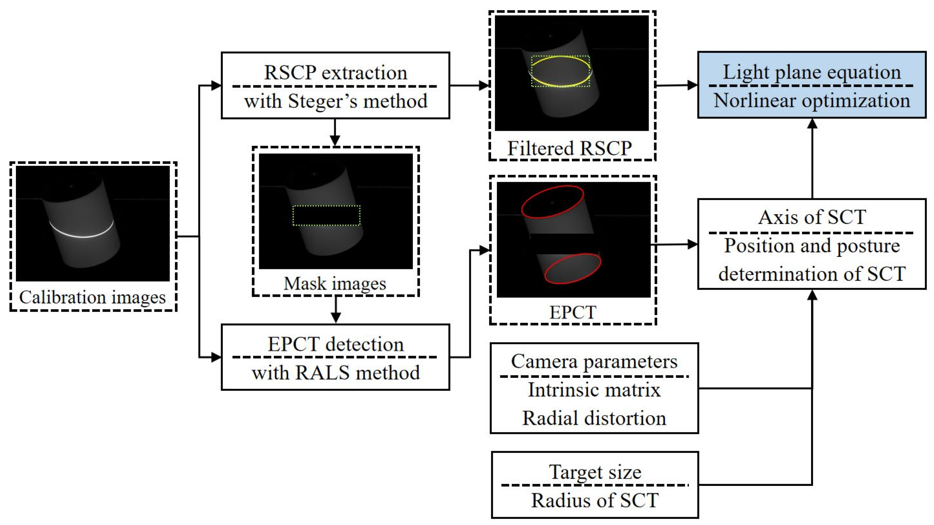
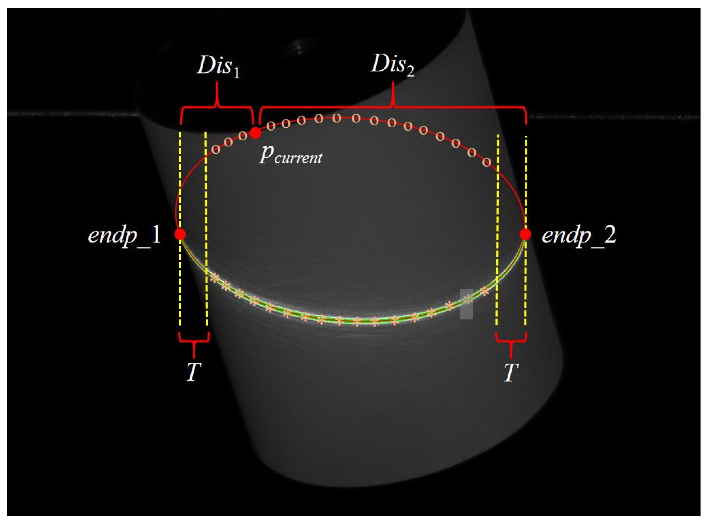
3.1. Calibration-Image Processing

Figure 3 shows a captured image of the SCT during calibration. In the calibration-image processing, there are two contents: (1) the RSCP must be extracted, (2) the EPCT need to be detected. Because of high brightness and contrast of the light stripe, the first content is to process the light stripe with Steger’s method [28], and there are three main steps.

Step 1. Image preprocessing and solving the normal vector:

In order to approximate the ideal model of the light-stripe section, a Gaussian filter is applied to preprocess the image. In addition, the normal vector of the center line of the light stripe is solved through the Hessian matrix.

Step 2. Determining the subpixel points:

The gray distribution function is obtained by Taylor polynomial expansion along the normal vector, and then the subpixel centerpoints of the light stripe are determined.

Step 3. Refining the subpixel points:

According to the theoretical derivation (see Appendix A), the subpixel points should be on an ellipse. Thus, the subpixel points can be fitted to an ellipse, and then the ellipse is resampled to obtain refined subpixel points, as shown in Figure 3a.

After the RSCP extraction, a minimum enveloping rectangular of the light stripe masks the current image to prevent the light stripe from affecting subsequent image processing. The second content is to detect the EPCT, and its purpose is ellipse detection. There are several conventional methods for ellipse detection, e.g., Hough transform [29] and edge-following [30] methods. Unfortunately, they have shortcomings of being less robust or more time-consuming. Therefore, a novel ellipse-detection method, which is called the RALS method [31], is introduced. The RALS method consists of two main steps:

Step 1. Initial ellipse-set generation:

According to the direction and polarity of the arc geometric cues, arc-support LS prunes the straight LS. Meanwhile, several arc-support LS that share the similar geometric properties are iteratively linked to form a group by satisfying the continuity and convexity conditions. The linked arc-support LS are called an “arc-support group”. Then, from the local and global perspectives, the initial ellipse set is generated from the arc-support groups. A detailed description can be found in ref. [32].

Step 2. Ellipse clustering and candidate determination:

Owing to the presence of duplicates in the initial ellipse, a hierarchical ellipse-clustering method [33] is proposed. Moreover, ellipse-candidate determination, which incorporates the stringent regulations for goodness measurements and elliptic geometric properties for refinement, is conducted. Finally, the EPCT are obtained, as shown in Figure 3b.

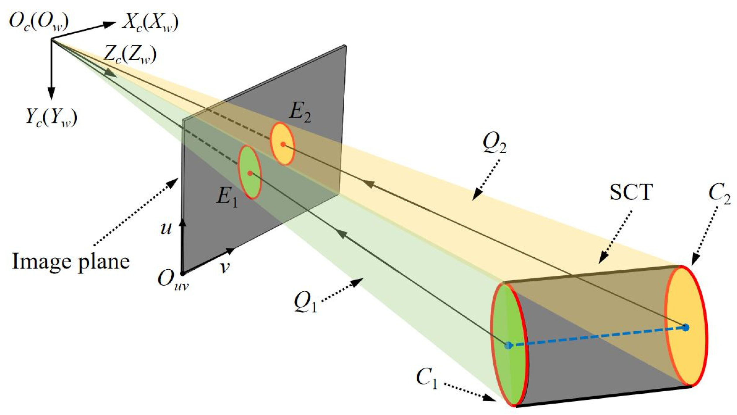
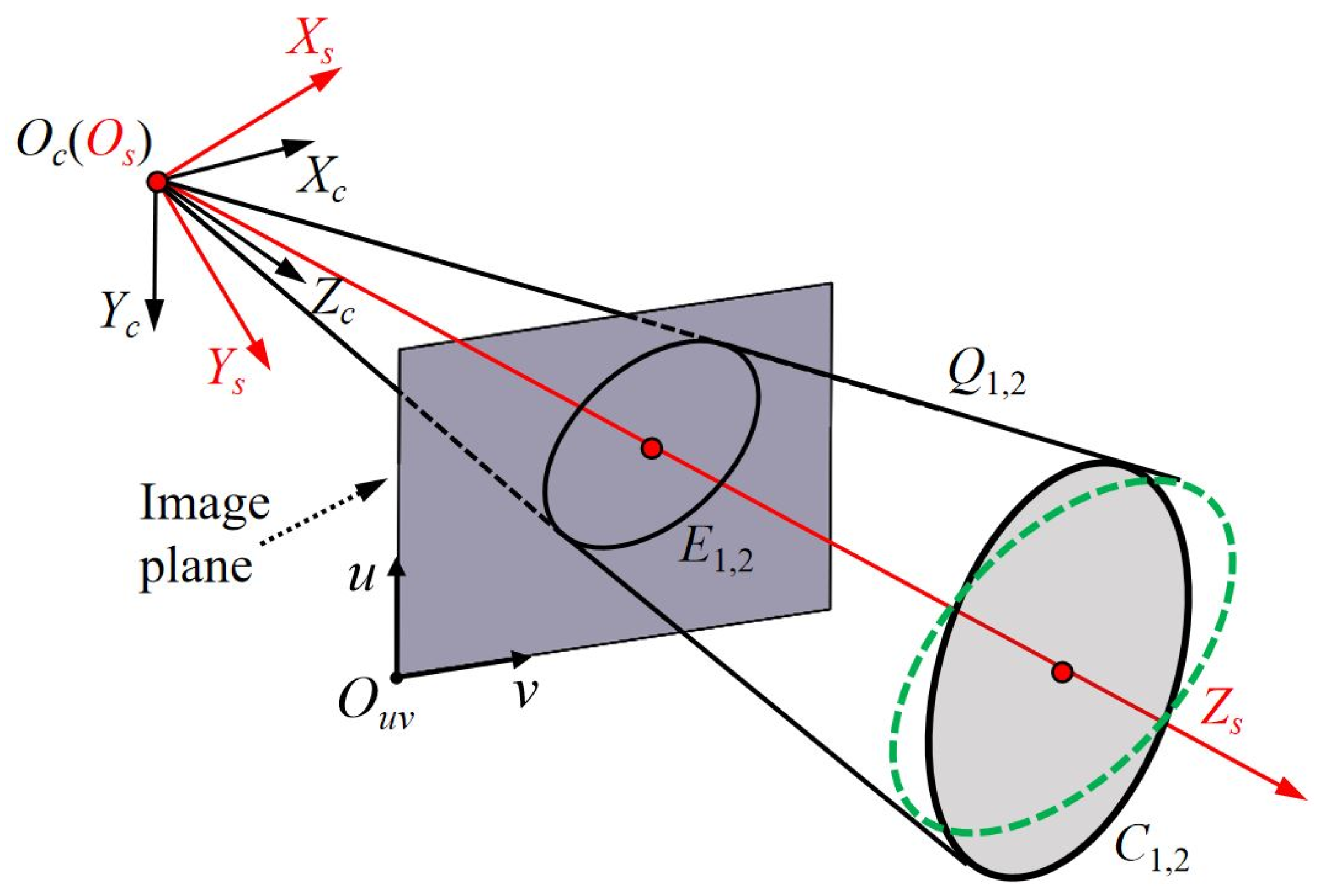
3.2. Position and Posture Determination of the SCT

According to space analytic geometry, if the radius of a cylinder is known, the axis equation of the cylinder can uniquely determine the cylinder. Therefore, the following focuses on the solution of the axis equation of the SCT. As shown in Figure 4, O_c is the optical center of the camera; (O_c; X_c, Y_c, Z_c) represents the CCS matching the WCS; (O_uv; u, v) is the camera pixel coordinate system (CPCS). The SCT is projected into the CPCS. The two end circles C_1,2 of the SCT in the CCS should correspond to the EPCT E_1,2 in the CPCS, and the equations of E_1,2 can be expressed as

$$a_{1,2}{u}_{1,2}^2+b_{1,2}{v}_{1,2}^2+c_{1,2}{u}_{1,2}{v}_{1,2}+d_{1,2}{u}_{1,2}+e_{1,2}{v}_{1,2}+f_{1,2}=0,$$

(4)

where (a_1,2, b_1,2, c_1,2, d_1,2, e_1,2, f_1,2) are the equation parameters of E_1,2, and (u_1,2, v_1,2) denote the pixel coordinates of E_1,2 in the CPCS. Equation (4) can also be rewritten as

$$\left(\begin{array}{ccc}{u}_{1,2}& v_{1,2}& 1\end{array}\right){\mathit{E}}_{1,2}\left(\begin{array}{c}{u}_{1,2}\\ v_{1,2}\\ 1\end{array}\right)=0.$$

(5)

E_1,2 denote a 3 × 3 symmetric matrix:

$${\mathit{E}}_{1,2}=\left[\begin{array}{ccc}{a}_{1,2}& c_{1,2}/2& d_{1,2}/2\\ c_{1,2}/2& b_{1,2}& e_{1,2}/2\\ d_{1,2}/2& e_{1,2}/2& f_{1,2}\end{array}\right].$$

(6)

Subsequently, E_1,2 and O_c can determine two elliptic cones, Q_1,2, whose equations can be solved by using the back-perspective projection model of the camera and are described as

$${\mathit{A}}_{1,2}{x}_{1,2}^2+B_{1,2}{y}_{1,2}^2+C_{1,2}{x}_{1,2}{y}_{1,2}+D_{1,2}{x}_{1,2}{z}_{1,2}+E_{1,2}{y}_{1,2}{z}_{1,2}+F_{1,2}{z}_{1,2}^2=0,$$

(7)

where (A_1,2, B_1,2, C_1,2, D_1,2, E_1,2, F_1,2) are the equation parameters of Q_1,2, and (x_1,2, y_1,2, z_1,2) denote the 3D coordinates of spatial points on Q_1,2 in the CCS. The above Equation (7) can also be rewritten as

$$\left(\begin{array}{ccc}{x}_{1,2}& y_{1,2}& z_{1,2}\end{array}\right){\mathit{W}}_{1,2}\left(\begin{array}{c}{x}_{1,2}\\ y_{1,2}\\ z_{1,2}\end{array}\right)=0.$$

(8)

W_1,2 denote a 3 × 3 symmetric matrix:

$${\mathit{W}}_{1,2}=\left[\begin{array}{ccc}{\mathit{A}}_{1,2}& C_{1,2}/2& D_{1,2}/2\\ C_{1,2}/2& B_{1,2}& E_{1,2}/2\\ D_{1,2}/2& E_{1,2}/2& F_{1,2}\end{array}\right].$$

(9)

According to the back-perspective projection, the following relation can be established:

$${\mathit{A}}_{\mathbf{I}}^T{\mathit{E}}_{1,2}{\mathit{A}}_{\mathit{I}}=\left[\begin{array}{cc}{\mathit{W}}_{1,2}& 0\\ 0& 0\end{array}\right],$$

(10)

where A_I = A[I 0] represents the auxiliary camera matrix, and A is the camera intrinsic matrix.

In order to simplify calculation, the CCS needs to be transformed to the standard coordinate system (SCS). As shown in Figure 5, (O_s; X_s, Y_s, Z_s) represents the SCS. The SCS and CCS have the same origin of the coordinate system. The Z_s axis points to the center of the end circle of the SCT. The X_s and Y_s axis conform to the right-handed coordinate system. Namely, the transformation between the SCS and CCS only involves rotation, and the relation can be expressed as

$$\left(\begin{array}{c}{x}_{1,2}\\ y_{1,2}\\ z_{1,2}\end{array}\right)={\mathit{R}}_{1,2}·\left(\begin{array}{c}{x}_{1,2}^{\prime }\\ y_{1,2}^{\prime }\\ z_{1,2}^{\prime }\end{array}\right),$$

(11)

where R_1,2 are the rotation matrixes of coordinate transformation, and ($x_{1,2}^{\prime },y_{1,2}^{\prime },z_{1,2}^{\prime }$) denote the 3D coordinates of spatial points on Q_1,2 in the SCS. Substituting Equation (11) into Equation (8), we can obtain

$$\left(\begin{array}{ccc}{x}_{1,2}^{\prime }& y_{1,2}^{\prime }& z_{1,2}^{\prime }\end{array}\right)·{\mathit{R}}_{1,2}^{-1}{\mathit{W}}_{1,2}{\mathit{R}}_{1,2}·\left(\begin{array}{c}{x}_{1,2}^{\prime }\\ y_{1,2}^{\prime }\\ z_{1,2}^{\prime }\end{array}\right)=0.$$

(12)

It is important to note that in order to transform Q_1,2 to the SCS, the following relationships should be satisfied:

$${\mathit{R}}_{1,2}^{-1}{\mathit{W}}_{1,2}{\mathit{R}}_{1,2}=\left[\begin{array}{ccc}{\lambda }_{a,1,2}& 0& 0\\ 0& {\lambda }_{b,1,2}& 0\\ 0& 0& {\lambda }_{c,1,2}\end{array}\right].$$

(13)

Hence, through solving the eigenvalue decomposition of W_1,2, we can obtain R_1,2 and the corresponding eigenvalues (λ_a,1,2, λ_b,1,2, λ_c,1,2). The equations of the elliptic cone Q_1,2 in the SCS can be written as

$${\lambda }_{a,1,2}{x}_{1,2}^{\prime 2}+{\lambda }_{b,1,2}{y}_{1,2}^{\prime 2}+{\lambda }_{c,1,2}{z}_{1,2}^{\prime 2}=0,$$

(14)

where the order of (λ_a,1,2, λ_b,1,2, λ_c,1,2) needs to be adjusted based on the following rules: (λ_a,1,2 < λ_b,1,2 < 0, λ_c,1,2 > 0) or (λ_a,1,2 > λ_b,1,2 > 0, λ_c,1,2 < 0).

As shown in Figure 5, it should be noted that there are two planes that intersect the elliptic cones Q_1,2 to form the circles C_1,2 (i.e., green dotted and black solid circles) with the radius R of the SCT. In ref. [34], the expressions of the center and normal vector of C_1,2, which are related to (λ_a,1,2, λ_b,1,2, λ_c,1,2) and R, are reported.

$$\{\begin{array}{l}\left(x_{axis,1,2}^{\prime },y_{axis,1,2}^{\prime },z_{axis,1,2}^{\prime }\right)=\left(\pm R\sqrt{\frac{\left|{\lambda }_{c,1,2}\right|\left(\left|{\lambda }_{a,1,2}\right|-\left|{\lambda }_{b,1,2}\right|\right)}{\left|{\lambda }_{a,1,2}\right|\left(\left|{\lambda }_{a,1,2}\right|+\left|{\lambda }_{c,1,2}\right|\right)}},0,R\sqrt{\frac{\left|{\lambda }_{a,1,2}\right|\left(\left|{\lambda }_{b,1,2}\right|+\left|{\lambda }_{c,1,2}\right|\right)}{\left|{\lambda }_{c,1,2}\right|\left(\left|{\lambda }_{a,1,2}\right|+\left|{\lambda }_{c,1,2}\right|\right)}}\right)\hfill \\ \left(n_{axis,x,1,2}^{\prime },n_{axis,y,1,2}^{\prime },n_{axis,z,1,2}^{\prime }\right)=\left(\pm \sqrt{\frac{\left|{\lambda }_{a,1,2}\right|-\left|{\lambda }_{b,1,2}\right|}{\left|{\lambda }_{a,1,2}\right|+\left|{\lambda }_{c,1,2}\right|}},0,-\sqrt{\frac{\left|{\lambda }_{b,1,2}\right|+\left|{\lambda }_{c,1,2}\right|}{\left|{\lambda }_{a,1,2}\right|+\left|{\lambda }_{c,1,2}\right|}}\right)\hfill \end{array},$$

(15)

where ($x_{axis,1,2}^{\prime },y_{axis,1,2}^{\prime },z_{axis,1,2}^{\prime }$) and ($n_{axis,x,1,2}^{\prime },n_{axis,y,1,2}^{\prime },n_{axis,z,1,2}^{\prime }$) express the center coordinates and normal vector of C_1,2, respectively. Obviously, Equation (15) is ambiguous, and cannot calculate the axis equation of the SCT. Fortunately, the SCT has two end circles, whose normal vectors are the same. Therefore, the center coordinates and normal vectors of C_1,2 can be uniquely determined. Next, in order to unify the coordinate system, ($x_{axis}^{\prime },y_{axis}^{\prime },z_{axis}^{\prime }$) and ($n_{axis,x}^{\prime },n_{axis,y}^{\prime },n_{axis,z}^{\prime }$) need to be converted back into the CCS according to the following relationships:

$$\{\begin{array}{l}\left(\begin{array}{c}{x}_{axis,1,2}\\ y_{axis,1,2}\\ z_{axis,1,2}\end{array}\right)={\mathit{R}}_{1,2}\left(\begin{array}{c}{x}_{axis,1,2}^{\prime }\\ y_{axis,1,2}^{\prime }\\ z_{axis,1,2}^{\prime }\end{array}\right)\hfill \\ \left(\begin{array}{c}{n}_{axis,x,1,2}\\ n_{axis,y,1,2}\\ n_{axis,z,1,2}\end{array}\right)={\mathit{R}}_{1,2}\left(\begin{array}{c}{n}_{axis,x,1,2}^{\prime }\\ n_{axis,y,1,2}^{\prime }\\ n_{axis,z,1,2}^{\prime }\end{array}\right)\hfill \end{array}.$$

(16)

For more precision, the axis vector of the SCT is taken as the average of the vector formed by the centers of C_1,2 and the normal vectors of C_1,2. The midpoint of the center coordinates of C_1,2 serves as a special point on the axis of the SCT. The expression is written as:

$$\{\begin{array}{l}\left(\begin{array}{ccc}{x}_{axis}& y_{axis}& z_{axis}\end{array}\right)=\mathrm{mean}\left[\left(\begin{array}{ccc}{x}_{axis,1}& y_{axis,1}& z_{axis,1}\end{array}\right),\left(\begin{array}{ccc}{x}_{axis,2}& y_{axis,2}& z_{axis,2}\end{array}\right)\right]\hfill \\ \left(\begin{array}{ccc}{n}_{axis,x}& n_{axis,y}& n_{axis,z}\end{array}\right)=\mathrm{mean}\left[\begin{array}{l}\left(\begin{array}{ccc}{x}_{axis,1}-x_{axis,2}& y_{axis,1}-y_{axis,2}& z_{axis,1}-z_{axis,2}\end{array}\right),\\ \left(\begin{array}{ccc}{n}_{axis,x,1}& n_{axis,y,1}& n_{axis,z,1}\end{array}\right),\\ \left(\begin{array}{ccc}{n}_{axis,x,2}& n_{axis,y,2}& n_{axis,z,3}\end{array}\right)\end{array}\right]\hfill \end{array},$$

(17)

where mean [.] represents average operator, and (x_axis, y_axis, z_axis) and (n_axis,x, n_axis,y, n_axis,z) are a special point on the axis and the axis vector of the SCT, respectively. Finally, the axis equation of the cylindrical target can be expressed as

$$\frac{x_c-x_{axis}}{n_{axis,x}}=\frac{y_c-y_{axis}}{n_{axis,y}}=\frac{z_c-z_{axis}}{n_{axis,z}}.$$

(18)

3.3. Nonlinear Optimization of the Light-Plane Equation

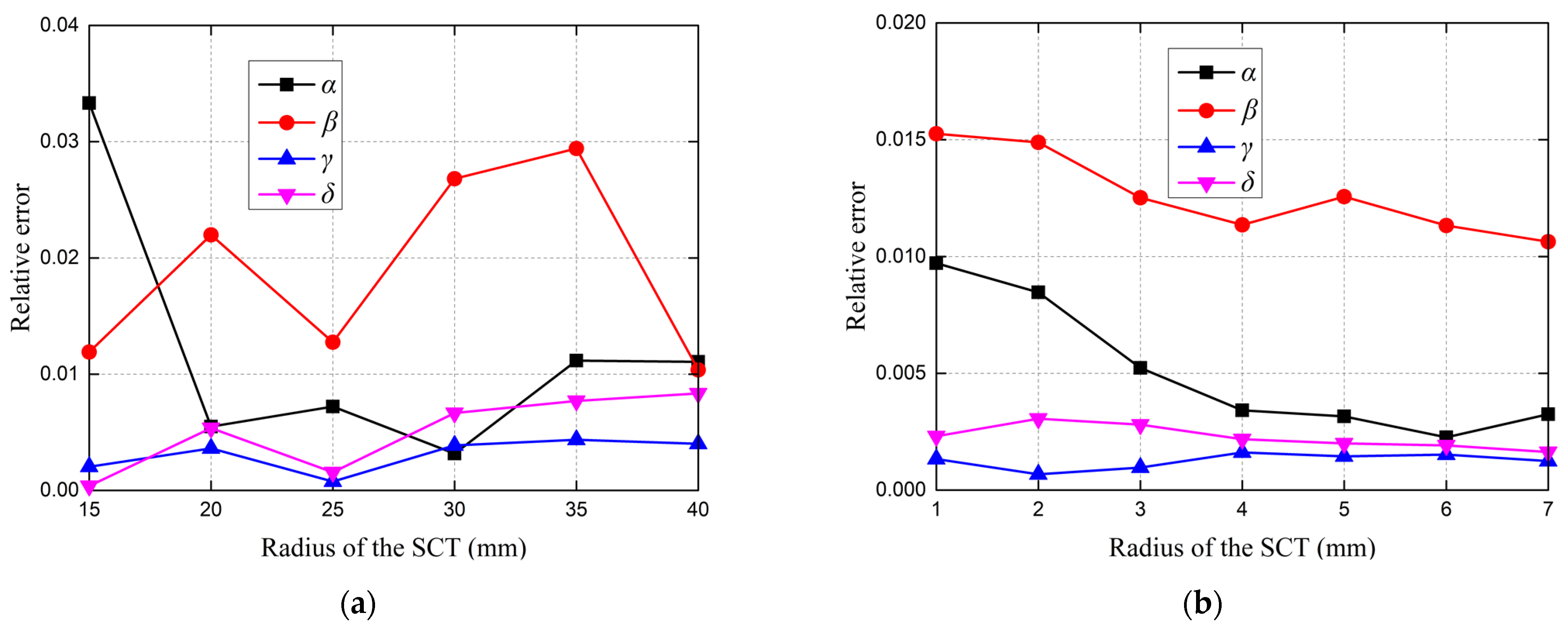
According to Section 3.1, the RSCP of the light stripe is extracted. The coordinates of the RSCP should satisfy the following camera model:

$${\mathit{A}}^{-1}·\left(\begin{array}{c}{u}_{RSCP}\\ v_{RSCP}\\ 1\end{array}\right)=\left(\begin{array}{c}{x}_{c,RSCP}\\ y_{c,RSCP}\\ z_{c,RSCP}\end{array}\right),$$

(19)

where (u_RSCP, v_RSCP) represents the coordinates of the RSCP in the CPCS, and (x_c,RSCP, y_c,RSCP, z_c,RSCP) denotes the coordinates of the corresponding points of the RSCP on the intersection of the light plane and the SCT in the CCS.

The distance from the points (x_c,RSCP, y_c,RSCP, z_c,RSCP) to the axis of the cylindrical target should be the radius R of the SCT, i.e., there is the following relation:

$${\left[\left(\begin{array}{c}{x}_{c,RSCP}-x_{axis}\\ y_{c,RSCP}-y_{axis}\\ z_{c,RSCP}-z_{axis}\end{array}\right)\times \left(\begin{array}{c}{n}_{axis,x}\\ n_{axis,y}\\ n_{axis,y}\end{array}\right)\right]}^2=R^2.$$

(20)

Essentially, Equation (20) expresses a cylinder equation. By combining Equations (19) and (20), the coordinates (x_c,RSCP, y_c,RSCP, z_c,RSCP) can be solved. However, there is a phenomenon that needs to be highlighted and specifically addressed: From the geometric viewpoint, Equation (19) is a ray equation. If a ray intersects a cylinder, there should be two points of intersection (e.g., p₁ and p₂ in Figure 6). Obviously, one of both (e.g., p₂ in Figure 6) is not in the light plane. In other words, if our proposed method is used directly, two solutions for p₁ and p₂ can be obtained, which will cause ambiguity.

Here, we devise a strategy to eliminate the ambiguity. Figure 7 is taken as an example to illustrate. Firstly, two endpoints (endp_1 and endp_2) of the light stripe are extracted. Then, the label of the current point p_current on the RSCP is determined based on the following policy:

$$\begin{array}{l}if\left(p_{current}\mathrm{is}\mathrm{on}\mathrm{the}\mathrm{light}\mathrm{stripe}\right)\&\left(Di{s}_{1,2}>T\right)\\ \mathrm{flag}=0;\\ elseif\left(p_{current}\mathrm{is}\mathrm{not}\mathrm{on}\mathrm{the}\mathrm{light}\mathrm{stripe}\right)\&\left(Di{s}_{1,2}>T\right)\\ \mathrm{flag}=1;\end{array}$$

where Dis_1,2 represent the distances from p_current to endp_1 and endp_2, and T is a threshold used to enhance robustness. “flag” represents the label of p_current. Next, there is iteration over all points in the RSCP and labels are marked. The points of flag = 0 correspond to the points on the intersection of the light plane and the cylindrical target, and these points are expressed as asterisks. Similarly, the points of flag = 1 and their corresponding points are expressed as circles. From the measurement-system layout, the corresponding points of flag = 0 on the intersection are closer to the camera. Therefore, when flag = 0, the coordinates of the current point should be the ones with the smaller z-coordinate value; and when flag = 1, vice versa.

After the coordinates on the intersection of the light plane and the SCT calculation, the following optimal objective function, which minimizes the distance from the points to the light plane, is established:

$$\mathrm{plane}(\alpha ,\beta ,\gamma ,\delta )=\min \left({\displaystyle \sum _i^n{\displaystyle \sum _j^m\frac{\alpha x_{c,RSCP,i,j}+\beta y_{c,RSCP,i,j}+\gamma z_{c,RSCP,i,j}+\delta }{\sqrt{{\alpha }^2+{\beta }^2+{\gamma }^2}}}}\right)$$

(21)

where (x_c,RSCP,i,j, y_c,RSCP,i,j, z_c,RSCP,i,j) denote the coordinates of the jth point on the intersection of the light plane and the cylindrical target when the cylindrical target is placed at the ith position in the CCS. The optimal solution of Equation (21) is derived through a nonlinear procedure (e.g., Levenberg–Marquardt).

4. Simulations

This section simulates the influences of the number of target placements and cylindrical-target radiuses on the calibration accuracy. In the simulation, the lens focus is set to 8 mm, the camera resolution is 1280 pixels × 960 pixels, and the pixel size of the image sensor is 3.75 um × 3.75 um. The simulated light-plane equation is −0.2500x + 0.2588y − 0.9330z + 320.9310 = 0. The calibration accuracy is evaluated with the relative errors of the coefficients of the light-plane equation.

Simulation 1. 

Influence of cylindrical-target radiuses.

Gaussian noise (σ = 0.2 pixels) is incorporated into the simulated calibration images. The cylindrical target is placed twice, and its radius varies from 15 to 40 mm at an interval 5 mm. The relative errors of the coefficients and the average relative error at different target radiuses are presented in Figure 8a. The curves (especially the average relative error) show that the error decreases with increasing target radiuses from 15 to 25 mm, and is almost constant at a target radius above 25 mm. Therefore, considering economy, a SCT with a radius of 25 mm is manufactured and used in the physical experiment.

Simulation 2. 

Inference of the number of target placements.

The number of target placements is varied from 1 to 7. The radius of the target is set to 25 mm, and the noise level is σ = 0.2 pixels. Figure 8b depicts the relative error curves of the coefficients at different placement numbers, and clearly shows that calibration accuracy increases with the increasing number of target placements. In addition, the relative error tends to stabilize when the number of target placements reaches four. Thus, considering efficiency, the number of target placements can be set to four in the physical experiment.

5. Experiments

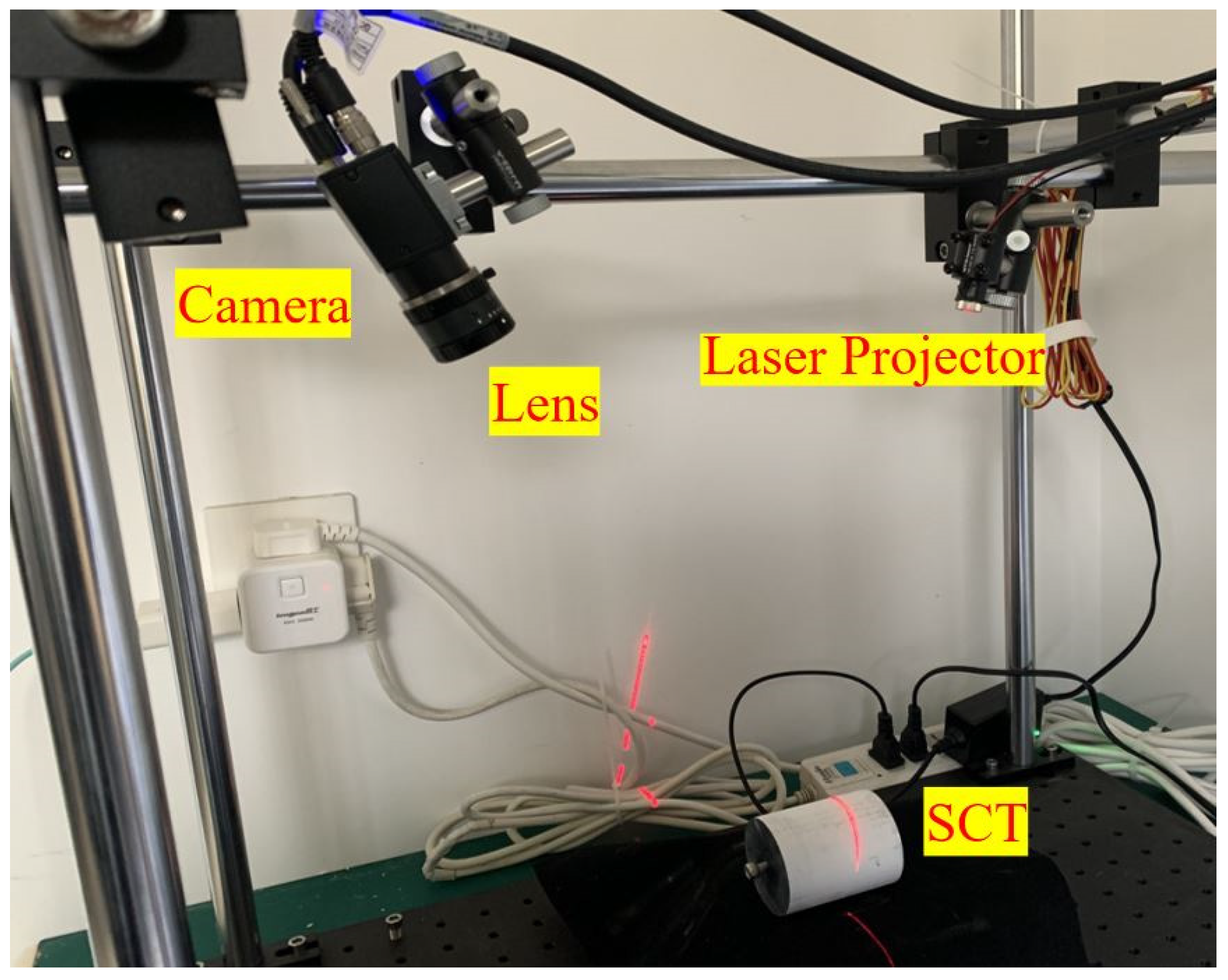
5.1. Experimental-System Setup

The experimental system is composed of a digital charge-coupled device (CCD) camera (MV-CE013-50GM) and a laser projector. The CCD camera (resolution 1280 pixels × 960 pixels) attaches to an 8 mm focal-length megapixel lens (Computer MP0814-MP2). The laser projector casts a single-line laser (minimum linewidth 0.2 mm). The radius of the cylindrical target is 25 mm, and its accuracy of manufacture is 0.01 mm. The measurement distance of the system is approximately 350 mm. Figure 9 displays the experimental-system setup.

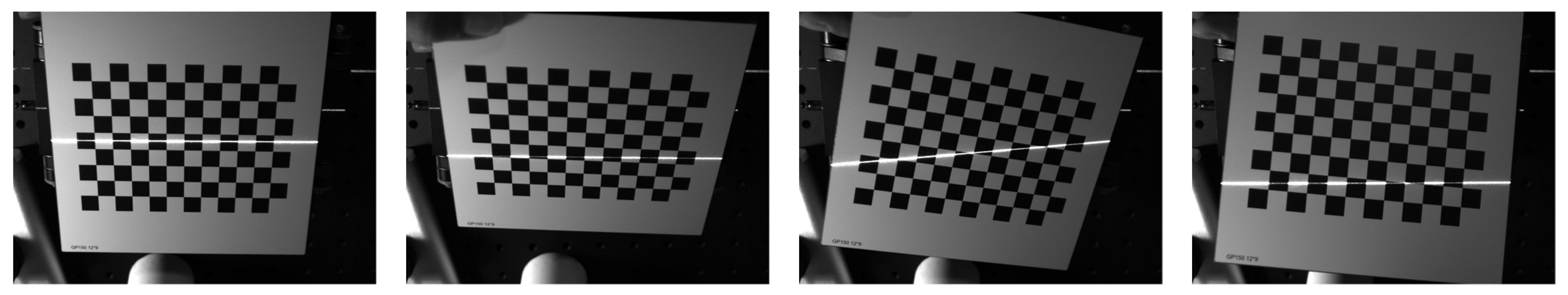
5.2. Experimental Procedure

Step 1: The camera intrinsic matrix and the radial distortion parameters are obtained through utilizing the MATLAB toolbox provided by Bouguet [35]: k₁ = −0.1006, k₂ = 0.1506 and

$$\mathit{A}=\left[\begin{array}{ccc}2223.4912& 0& 6493.2807\\ 0& 2223.9354& 526.1537\\ 0& 0& 1\end{array}\right].$$

Step 2: The camera captures a calibration image when the cylindrical target is placed at an appropriate position. Meanwhile, the captured image is undistorted. Then, according to the calibration-image processing in Section 3.1, the RSCP is extracted, and the EPCT are detected.

Step 3: As described in Section 3.2, combining the obtained EPCT, the calibrated camera parameters, and the known radius of the SCT, the axis equation of the SCT at the current position is solved.

Step 4: The coordinates of the corresponding points in the RSCP on the intersection of the light plane and the SCT in the CCS are calculated through utilizing the camera model [see Equation (19)] and the cylindrical equation [see Equation (20)].

Step 5: Step 2 to 4 are repeated. The camera captures several calibration images when the SCT is placed at other positions. Several groups of the coordinates of the corresponding points in the RSCP are obtained after Step 4. Then, by using these points, the light-plane equation is nonlinearly optimized.

5.3. Comparison Evaluation

In order to verify the effectiveness of our proposed method, a comparative evaluation experiment was performed between the method proposed in ref. [20] and our proposed method. First, the experimental system was calibrated with the method proposed in ref. [20]. A chessboard as a two-dimensional calibration target was placed at the appropriate position four times. The size of the grid is 10 mm × 10 mm and its accuracy of manufacture is 0.01 mm. The four calibration images are shown in Figure 10. The calibration result is

$$0.0029x-0.7712y-0.6366z+220.7429=0.$$

(22)

Then, the experimental system was calibrated with our proposed method. The cylindrical target was placed at the appropriate position four times. The calibration images are shown in Figure 11. We calculated the light-plane equations when the cylindrical target was at one time (one of four times selected) and four times, and their calibration results, respectively, are

$$0.0035x-0.7731y-0.6358z+220.6950=0,$$

(23)

$$0.0033x-0.7727y-0.6360z+220.5770=0.$$

(24)

Finally, we selected four images, which contained light stripes, to verify the effectiveness. Four measurement points need be specified on the light stripe of each image. The coordinates of these measurement points were calculated with the line-structured light 3D-measurement model. It is noted that the light-plane equations of the model were respectively calculated with Zhou’s method and our proposed methods (one time and four times), i.e., Equations (22)–(24). The calculated results are listed in

Table 1. 3D coordinates of four measurement points on four images computed with Zhou’s method and our proposed methods (one time and four times), respectively (Unit: mm).

Img. No.	Pt. No.	3D Coordinates with Zhou’s Method			3D Coordinates with Our Proposed Method (One Time)			3D Coordinates with Our Proposed Method (Four Times)
1	1	−64.8947	−6.1514	353.9093	−64.9559	−6.1572	354.2431	−64.9035	−6.1522	353.9570
	2	−30.0231	−6.3441	354.3015	−30.0544	−6.3507	354.6705	−30.0291	−6.3453	354.3725
	3	5.8525	−6.3470	354.4686	5.8592	−6.3543	354.8726	5.8541	−6.3487	354.5629
	4	49.2086	−6.3507	354.6705	49.2706	−6.3587	355.1169	49.2256	−6.3529	354.7929
2	1	−62.6991	−9.7994	358.3387	−62.7616	−9.8092	358.6959	−62.7101	−9.8012	358.4016
	2	−19.1331	−1.8554	348.9135	−19.1524	−1.8573	349.2668	−19.1364	−1.8557	348.9745
	3	15.3191	4.2758	341.6428	15.3349	4.2802	341.9938	15.3218	4.2766	341.7029
	4	51.4641	10.4954	334.2729	51.5179	10.5063	334.6223	51.4733	10.4973	334.3328
3	1	−66.7849	6.8915	338.1001	−66.8362	6.8968	338.3598	−66.7844	6.8915	338.0978
	2	−45.9074	12.9892	330.8081	−45.9417	12.9989	331.0549	−45.9058	12.9888	330.7964
	3	−23.9047	4.4499	341.2532	−23.9267	4.4540	341.5663	−23.9071	4.4504	341.2868
	4	−30.6853	9.4680	335.1432	−30.7109	9.4759	335.4226	−30.6863	9.4683	335.1536
4	1	−79.4441	−53.2654	410.9187	−79.7660	−53.4812	412.5834	−79.4944	−53.2991	411.1786
	2	−40.6191	1.4219	344.8453	−40.7086	1.4251	345.6052	−40.6232	1.4221	344.8802
	3	−27.2117	7.2410	337.8570	−27.2590	7.2535	338.4440	−27.2134	7.2414	337.8778
	4	−3.4644	7.0703	338.1719	−3.4680	7.0778	338.5268	−3.4647	7.0711	338.2080

. The first and second columns express the image and point number, respectively. The 3D coordinates of the four measurement points on four images, calculated with Zhou’s method and our proposed methods (one time and four times), respectively, are shown from the third to fifth columns in Table 1. Furthermore, the result of Table 1 shows that (1) the light plane can be calibrated with our proposed method when the calibration target is at one time; (2) the effectiveness of light-plane calibration with our proposed method and the comparison method is approximate and unanimous when the calibration target is at four times.

5.4. Accuracy Evaluation

In order to verify the accuracy of our proposed method, an accuracy-evaluation experiment was performed between our proposed method and the methods proposed in refs. [20,27]. The chessboard was placed inside the measured volume, and its external parameter could be obtained. O_T is the origin of the chessboard. The coordinates of O_T in the target coordinate system (TCS) are (0, 0, 0), and in the CCS can be solved according to the external parameter of chessboard. Here, the principle of cross-ratio invariance (CRI) is introduced to calculate the coordinates of the point D in the target coordinate system (TCS). The distance d_t (from D to O_T in the TCS) is considered as the ideal evaluation distance. Meanwhile, the coordinates of the testing point D in the CCS were also calculated with the light-structured light 3D-measurement model, where the light-plane equations were respectively solved with Zhou’s method [20], Zhu’s method [27], and our proposed methods (one time and four times). Similarly, the distance d_m (from D to O_T in the CCS) are measured distances. The coordinates of the ideal points and the testing points are listed in

Table 2. 3D coordinates of the ideal points and testing points (Unit: mm).

Img. No.	3D Coordinates of CRI in the TCS			3D Coordinates of Testing Points with Zhou’s Method			3D Coordinates of Testing Points with Zhu’s Method			3D Coordinates of Testing Points with Our Proposed Method (One Time)			3D Coordinates of Testing Points with Our Proposed Method (Four Time)
1	35.3298	50	0	7.5092	3.3665	342.7088	7.4988	3.3567	343.3210	7.5168	3.3700	343.0576	7.5104	3.3671	342.7673
	35.4605	70	0	26.7451	6.9766	338.4231	26.7235	6.9654	338.5439	26.7725	6.9837	338.7694	26.7496	6.9778	338.4804
2	45.5751	30	0	−8.8570	7.2698	337.9057	−8.8498	7.2659	338.1598	−8.8651	7.2765	338.2172	−8.8579	7.2705	337.9400
	44.7668	60	0	21.2191	7.5686	337.6807	21.2145	7.5839	338.1210	21.2403	7.5762	338.0185	21.2224	7.5698	337.7325
3	35.5497	30	0	−18.8642	−6.5621	354.7166	−18.8598	−6.5705	355.0120	−18.8684	−6.5636	354.6956	−18.8844	−6.5692	354.9977
	36.0057	70	0	21.1461	−6.5656	354.8030	21.1821	−6.5801	355.1356	21.1712	−6.5734	355.2233	21.1524	−6.5675	354.9081

, i.e., the second column shows the 3D coordinates of CRI in the TCS, which is regarded as 3D data of the ideal points; and the 3D coordinates of testing points with Zhou’s method, Zhu’s method, and our proposed methods (one time and four times), respectively, are shown from the third to sixth columns. The distance data and the corresponding accuracy-analysis results are shown in

Table 3. Statical results of the Table 2. (Unit: mm).

Img. No.	dt	dm1	dm2	dm3	dm4	Δ(dt, dm1)	Δ(dt, dm2)	Δ(dt, dm2)	Δ(dt, dm3)
1	61.2225	61.2170	61.2626	61.2583	61.2238	0.0055	0.0401	−0.0358	−0.0013
	78.4694	78.4230	78.4011	78.4566	78.4285	0.0464	−0.0683	0.0128	0.0409
2	54.5627	54.6404	54.6696	54.6774	54.6443	−0.0777	0.1069	−0.1147	−0.0816
	74.8603	74.8623	74.9039	74.9106	74.8697	−0.0020	0.0436	−0.0503	−0.0094
3	46.5165	46.4330	46.5333	46.4220	46.5131	0.0835	0.0168	0.0945	0.0034
	78.7173	78.6527	78.7481	78.7595	78.6793	0.0646	0.0308	−0.0422	0.0380
RMS error						0.0568	0.0589	0.0681	0.0406

, where the d_t column represents the ideal evaluation distance and the d_m1…4 columns show the measured distances with Zhou’s method, Zhu’s method, and our proposed methods (one time and four times), respectively. The last four columns are absolute errors (between d_m1…4 and d_t), and their corresponding root-mean-square (RMS) errors. In Table 3, using Zhou’s method, Zhu’s method, and our proposed methods (one time and four times), the root-mean-square (RMS) errors are 0.0568 mm, 0.0589 mm, 0.0681 mm, and 0.0406 mm, respectively. The calibration accuracy with our proposed method is comparable to that with the method of the chessboard target (i.e., Zhou’s method) and the SCT under non-free posture (i.e., Zhu’s method).

6. Conclusions

In this study, a novel calibration method for a line-structured light 3D-measurement method based on an SCT is proposed. The SCT can be easily manufactured and move freely in calibration processing. In calibration-image processing, the RSCP are extracted with Steger’s method and the EPCT are detected with the RALS method. Combining two defined elliptical cones, which are defined by the two end circles of the SCT and the camera optical center, and the known radius of the SCT, the axis equation of the SCT is solved. Based on the camera model and the cylindrical equation, the coordinates of RSCP in the CCS can calculated to nonlinearly optimize the light-plane equation. The effectiveness of the proposed method is verified by simulations and experiments, and its calibration accuracy (RMS value) is about 0.04 mm.

References

1. Tang, Y.; Li, L.; Wang, C.; Chen, M.; Feng, W.; Zou, X.; Huang, K. Real-time detection of surface deformation and strain in recycled aggregate concrete-filled steel tubular columns via four-ocular vision. Robot. Comput.-Integr. Manuf. 2019, 59, 36–46. [Google Scholar] [CrossRef]
2. Tang, Y.; Chen, M.; Wang, C.; Luo, L.; Li, J.; Lian, G.; Zou, X. Recognition and Localization Methods for Vision-Based Fruit Picking Robots: A Review. Front. Plant Sci. 2020, 11, 510. [Google Scholar] [CrossRef] [PubMed]
3. Manzo, M.; Pellino, S. FastGCN + ARSRGemb: A novel framework for object recognition. J. Electron. Imaging 2021, 30, 033011. [Google Scholar] [CrossRef]
4. Liu, Z.; Li, F.; Huang, B.; Zhang, G. Real-time and accurate rail wear measurement method and experimental analysis. J. Opt. Soc. Am. A 2014, 31, 1721–1729. [Google Scholar] [CrossRef]
5. Jiang, J.; Miao, Z.; Zhang, G.J. Dynamic altitude angle measurement system based on dot-structure light. Infrared Laser Eng. 2010, 39, 532–536. [Google Scholar]
6. Zhang, G.; Liu, Z.; Sun, J.; Wei, Z. Novel calibration method for a multi-sensor visual measurement system based on structured light. Opt. Eng. 2010, 49, 043602. [Google Scholar] [CrossRef]
7. Li, X.; Zhang, W. Binary defocusing technique based on complementary decoding with unconstrained dual projectors. J. Eur. Opt. Soc-Rapid. 2021, 17, 14. [Google Scholar] [CrossRef]
8. Zuo, C.; Feng, S.; Huang, L.; Tao, T.; Yin, W.; Chen, Q. Phase shifting algorithms for fringe projection profilometry: A review. Opt. Laser Eng. 2018, 109, 23–59. [Google Scholar] [CrossRef]
9. Sam, V.; Dirckx, J. Real-time structured light profilometry: A review. Opt. Laser Eng. 2016, 87, 18–31. [Google Scholar]
10. Li, Y. Single-mirror beam steering system: Analysis and synthesis of high-order conic-section scan patterns. Appl. Opt. 2008, 87, 386–398. [Google Scholar] [CrossRef]
11. Duma, V.F. Laser scanners with oscillatory elements: Design and optimization of 1D and 2D scanning functions. Appl. Math. Model. 2019, 67, 456–476. [Google Scholar] [CrossRef]
12. Xu, X.B.; Fei, Z.W.; Yang, J.; Tan, Z.; Luo, M. Line structured light calibration method and centerline extraction: A review. Results Phys. 2020, 19, 103637. [Google Scholar] [CrossRef]
13. Zhang, Z.Y. A Flexible New Technique for Camera Calibration. IEEE Trans. Pattern Anal. Mach. Intell. 2000, 22, 1330–1334. [Google Scholar] [CrossRef] [Green Version]
14. Huang, L.; Da, F.; Gai, S. Research on multi-camera calibration and point cloud correction method based on three-dimensional calibration object. Opt. Lasers Eng. 2019, 115, 32–41. [Google Scholar] [CrossRef]
15. Liu, X.S.; Li, A.H. An integrated calibration technique for variable-boresight three-dimensional imaging system. Opt. Lasers Eng. 2022, 153, 107005. [Google Scholar] [CrossRef]
16. Wang, Y.; Yuan, F.; Jiang, H.; Hu, Y. Novel camera calibration based on cooperative target in attitude measurement. Opt.-Int. J. Light Electron. Opt. 2016, 127, 10457–10466. [Google Scholar] [CrossRef]
17. Wong, K.Y.; Zhang, G.; Chen, Z. A stratified approach for camera calibration using spheres. IEEE Trans. Image Process. 2011, 20, 305–316. [Google Scholar] [CrossRef] [Green Version]
18. Wei, Z.; Cao, L.; Zhang, G. A novel 1D target-based calibration method with unknown orientation for structured light vision sensor. Opt. Laser Technol. 2010, 42, 570–574. [Google Scholar] [CrossRef]
19. Liu, C.; Sun, J.H.; Liu, Z.; Zhang, G. A field calibration method for line structured light vision sensor with large FOV. Opto-Electron. Eng. 2013, 40, 106–112. [Google Scholar]
20. Zhou, F.; Zhang, G. Complete calibration of a structured light stripe vision sensor through planar target of unknown orientations. Image Vis. Comput. 2005, 23, 59–67. [Google Scholar] [CrossRef]
21. Wang, P.; Wang, J.; Xu, J.; Zhang, G.; Chen, K. Calibration method for a large-scale structured light measurement system. Appl. Opt. 2017, 56, 3995–4002. [Google Scholar] [CrossRef] [PubMed]
22. Huynh, D.Q.; Owens, R.A.; Hartmann, P.E. Calibration a Structured Light Stripe System: A Novel Approach. Int. J. Comput. Vis. 1999, 33, 73–86. [Google Scholar] [CrossRef]
23. Xu, G.Y.; Li, L.F.; Zeng, J.C. A new method of calibration in 3D vision system based on structure-light. Chin. J. Comput. 1995, 18, 450–456. [Google Scholar]
24. Dewar, R. Self-generated targets for spatial calibration of structured light optical sectioning sensors with respect to an external coordinate system. Robot. Vis. Conf. Proc. 1988, 1, 5–13. [Google Scholar]
25. Liu, Z.; Li, X.; Li, F.; Zhang, G. Calibration method for line-structured light vision sensor based on a single ball target. Opt. Lasers Eng. 2015, 69, 20–28. [Google Scholar] [CrossRef]
26. Liu, Z.; Li, X.; Yin, Y. On-site calibration of line-structured light vision sensor in complex light environments. Opt. Express 2015, 23, 29896–29911. [Google Scholar] [CrossRef]
27. Zhu, Z.M.; Wang, X.Y.; Zhou, F.Q.; Cen, Y.G. Calibration Method for Line-Structured Light Vision Sensor based on a Single Cylindrical Target. Appl. Opt. 2019, 59, 1376–1382. [Google Scholar] [CrossRef]
28. Steger, C. An unbiased detector of curvilinear structures. IEEE Trans. Pattern Anal. 1998, 20, 113–125. [Google Scholar] [CrossRef] [Green Version]
29. Tsuji, S.; Matsumoto, F. Detection of ellipses by a modified Hough transformation. IEEE Trans. Comput. 2006, 27, 777–781. [Google Scholar] [CrossRef]
30. Chia, A.Y.S.; Rahardja, S.; Rajan, D.; Leung, M.K. A split and merge based ellipse detector with self-correcting capability. IEEE Trans. Image Process. 2011, 20, 1991–2006. [Google Scholar] [CrossRef]
31. Lu, C.; Xia, S.; Shao, M.; Fu, Y. Arc-Support Line Segments Revisited: An Efficient High-Quality Ellipse Detection. IEEE Trans. Image Process. 2020, 29, 768–781. [Google Scholar] [CrossRef] [PubMed]
32. Paul, L.R. A note on the least squares fitting of ellipses. Pattern Recognit. Lett. 1993, 14, 799–808. [Google Scholar]
33. Kulpa, K. On the properties of discrete circles, rings, and disks. Comput. Graph. Image Process. 1979, 10, 348–365. [Google Scholar] [CrossRef]
34. Zhang, L.J.; Huang, X.X.; Feng, W.C.; Liang, S.; Hu, T. Solution of duality in circular feature with three line configuration. Acta Opt. Sin. 2016, 36, 51. [Google Scholar]
35. Bouguet, J.Y. Camera Calibration Toolbox Got MATLAB. 2015. Available online: http://www.vision.caltech.edu/bouguetj/calib_doc/ (accessed on 20 February 2022).
36. Bronshtein, I.N. Handbook of Mathematics; Springer: Berlin/Heidelberg, Germany, 2015. [Google Scholar]
Figure 1. Schematic diagram of the model for the line-structured light 3D measurement based on a SCT.
Photonics 09 00218 g001
Figure 2. Flowchart of our proposed calibration method.
Photonics 09 00218 g002
Figure 3. A calibration image of SCT. (a) RSCP are extracted by Steger’s method (i.e., the red elliptic curve); (b) EPCT are detected by RALS method (i.e., the two red elliptic curves).
Photonics 09 00218 g003
Figure 4. Schematic diagram of the position and posture determination of the SCT.
Photonics 09 00218 g004
Figure 5. Schematic diagram of diagonalization.
Photonics 09 00218 g005
Figure 6. Schematic diagram of the light beam passing through SCT.
Photonics 09 00218 g006
Figure 7. Schematic diagram of the strategy to eliminate ambiguity.
Photonics 09 00218 g007
Figure 8. Influence on the calibration accuracy. (a) Radius of the SCT; (b) placement times of the SCT.
Photonics 09 00218 g008
Figure 9. Experimental-system setup.
Photonics 09 00218 g009
Figure 10. Four calibration images of the chessboard used for Zhou’s method [16].
Photonics 09 00218 g010
Figure 11. Four calibration images of the SCT used for our proposed method.
Photonics 09 00218 g011