ADMM-SVNet: An ADMM-Based Sparse-View CT Reconstruction Network

Abstract

In clinical medical applications, sparse-view computed tomography (CT) imaging is an effective method for reducing radiation doses. The iterative reconstruction method is usually adopted for sparse-view CT. In the process of optimizing the iterative model, the approach of directly solving the quadratic penalty function of the objective function can be expected to perform poorly. Compared with the direct solution method, the alternating direction method of multipliers (ADMM) algorithm can avoid the ill-posed problem associated with the quadratic penalty function. However, the regularization items, sparsity transform, and parameters in the traditional ADMM iterative model need to be manually adjusted. In this paper, we propose a data-driven ADMM reconstruction method that can automatically optimize the above terms that are difficult to choose within an iterative framework. The main contribution of this paper is that a modified U-net represents the sparse transformation, and the prior information and related parameters are automatically trained by the network. Based on a comparison with other state-of-the-art reconstruction algorithms, the qualitative and quantitative results show the effectiveness of our method for sparse-view CT image reconstruction. The experimental results show that the proposed method performs well in streak artifact elimination and detail structure preservation. The proposed network can deal with a wide range of noise levels and has exceptional performance in low-dose reconstruction tasks.

1. Introduction

Computed tomography (CT) is a nondestructive testing method that is widely used in medical, industrial, and material applications as well as other fields. With its variety of applications in clinical medicine, the problem of X-ray radiation has aroused broad public concern [1,2]. Following the as low as reasonably achievable (ALARA) guidelines, researchers have aimed to use all kinds of techniques to reduce radiation doses while maintaining image quality [3]. There are two strategies for radiation dose reduction. One strategy is to minimize the X-ray flux by reducing the tube current and exposure time of the X-ray tube [4]. The other approach is to reduce the number of projection views [5]. In clinical medical applications, sparse-view CT is an effective method for realizing low-dose scanning. In this work, we focus on methods for obtaining high-quality images from sparse-view CT.

Sparse-view CT imaging methods can be divided into model-driven and data-driven strategies [6]. Model-driven methods include the analytical reconstruction method and the model-based iterative reconstruction method (MBIR). Analytical reconstruction methods, such as the traditional filter back-projection (FBP) algorithm, have been widely used in industrial and medical fields because of their fast speed [7]. However, the analytical method requires a high degree of completeness of the projection information. Due to the incomplete projection data on sparse-view CT, the method will produce severe streak artifacts, which will reduce the image quality. Compared with the traditional analytic algorithm, the MBIR algorithm integrates prior information, suppressing the artifacts when the projection data are incomplete. Therefore, the MBIR method is generally used when the projection data are incomplete. Classical MBIR algorithms include the algebraic reconstruction technique (ART) method [8], the simultaneous algebraic reconstruction technique (SART) method [9], and the expectation maximization (EM) method [10]. However, when the projection data are highly undersampled, the traditional MBIR algorithms have difficulty obtaining satisfactory results.

Although the MBIR reconstruction method has the advantage of eliminating artifacts, the regularization terms and parameters still need to be selected manually, which can be cumbersome. In recent years, with the continuous development of deep learning, data-driven methods have received a large amount of attention and made progress in many fields [11,12]. Boublil et al. [13] utilized a convolutional neural network (CNN) to integrate multiple reconstructed results. Wolterink et al. [14] proposed to train a noise-reducing generator CNN together with an adversarial discriminator CNN to reduce noise for low-dose CT. Jin et al. [15] proposed the FBPConvNet network, which combines the FBP algorithm with a deep CNN to solve ill-posed inverse problems. Chen et al. [16] used a residual code–decoder convolutional neural network (Red-CNN) for low-dose CT imaging. Zhang et al. [17] combined a gradient descent network with a deconvolution network to eliminate streak artifacts while maintaining a high degree of structural similarity. Kang et al. [18] proposed a deep CNN based on a directional wavelet. Yang et al. [19] used a generative adversarial network (GAN) to recover detailed information on images reconstructed by the FBP method. Zhang et al. [20] developed an initializer for the conjugate gradient algorithm. Although these deep learning methods have achieved good results, they are all a type of post-processing method. The relationship between the projection information and the reconstructed image information is not considered, which means that and the consistency of the data is ignored.

With the development of compressed sensing (CS) theory [21], reconstruction algorithms based on CS theory can now use image sparsity as prior information in the reconstruction. CS theory overcomes the limitations of the Nyquist sampling theorem and makes it possible to accurately reconstruct images from few projection data. The iterative algorithms based on CS mainly include methods based on total variation (TV) and dictionary learning. Using the sparsity of the l₁ norm of the image gradient (also known as the TV of the image), Sidky et al. [22] took the TV in the image as a regularization term and proposed the total variation–projection onto convex sets (TV-POCS) image reconstruction algorithm. Later, Sidky et al. [23] improved the algorithm and proposed the adaptive steepest descent projection onto convex sets (ASD-POCS) algorithm. To find a more suitable sparse transformation and sparse representation method for CT images, scholars proposed a method based on dictionary learning. By taking advantage of the fact that the image has a large amount of redundant information, the overcomplete dictionary [24] was used to obtain a sparse representation of the redundant information in the image. Chen et al. [25] combined dictionary learning with the TV method for magnetic resonance imaging (MRI) reconstruction and improved the image reconstruction quality. Xu et al. [26] incorporated the dictionary learning method into the objective function model to better retain the detailed information of the image. Although the reconstruction methods based on dictionary learning can obtain higher-quality images, they are difficult to generalize because of the large amount of computation.

To improve the reliability of the model, scholars have proposed the combination of model-driven and data-driven methods to promote the consistency of data for CT image reconstruction. The primary study on combining the data-driven model with the analytical model is that of Wurfl et al. [27], who mapped the FBP algorithm into a neural network, enabling joint learning of the compensation step projection and volume domain. Lee et al. [28] complemented the missing projection information based on a U-Net. Zhou et al. [29] proposed a cascading attention network of residual dense spatial channels capable of generating high-quality reconstruction results.

The combination of data-driven and MBIR models is a popular research topic among scholars. For example, Gupta et al. [30] used the projection gradient descent method to solve the least squares problem of the objective function and used a CNN to replace the projection operator in the projection gradient descent algorithm. The LEARN method proposed by Chen et al. [31] expands the iterative model into a deep learning network. Specifically, they combined a generalized regularization term as a priori knowledge with the least squares problem of the objective function and optimized it by applying a simple gradient descent method. The CNN was used to represent the gradient expansion of the generalized regularization term. All parameters except the system matrix were obtained by training, and the method showed excellent performance in terms of reconstruction quality.

The above methods directly solve the quadratic penalty function of the objective function. For inverse problems, there are many structural optimization problems in the calculation due to the large-scale and ill-posed nature of the problems in practice, and the ADMM is a better way to solve these problems [32]. The performance of the ADMM algorithm is higher, especially in the case of non-smooth regularization (such as the l₁ norm penalty function) [33]. Based on the advantages of the ADMM algorithm’s performance, Yang et al. [34,35] took the lead in developing the ADMM algorithm into a deep learning framework for MRI image reconstruction. The proposed deep ADMM-Net framework can learn the corresponding transforms, functions, and parameters adaptively. Li et al. [36] proposed a robust composite regularization model based on the ADMM-Net framework to exploit more prior knowledge and image features. For CT imaging, He et al. [37] used the same framework [34] for low-dose CT image reconstruction. Zhang et al. [38] unrolled the ADMM algorithm into a network and a mixed loss function was used to prevent images from being oversmoothed. Wang et al. [39] used the ADMM algorithm to decompose a regularization model to reduce artifacts and avoid the manual selection of parameters and regularization terms. These methods confirm the advantages of the model of the ADMM framework. The ADMM iterative model was used as the backbone architecture, and the key components were replaced by networks to avoid having to manually adjust the regularization terms, the sparsity transform, and the parameters. In particular, searching for the best transform domain is an active research area because a sparser representation usually leads to a higher reconstruction accuracy.

However, none of the above methods train the sparsity transform directly. In [38], the authors did not train the sparsity transform but fixed the sparsity transform to a tight wavelet frame. In [34,35,36], the authors only trained the coefficients of the DCT combination. In [37,39], the authors used a deep network to replace parts of the formula, such as the regularization term gradient [37], and a specific ADMM unfolding step [39]. Differently from the algorithms mentioned above, the proposed ADMM-SVNet network directly trains the most suitable sparse transform through the network, which increases the accuracy and robustness of the methods. In the training process, the sparsity transform and parameters are learned adaptively, thereby making the reconstruction network more accurate, effective, and robust.

The rest of the paper is organized as follows. Section 2 introduces the proposed reconstruction method. The experimental steps and results are described in Section 3 and Section 4, respectively. A discussion and our conclusions are presented in Section 5.

2. Methods

In this work, we aimed to perform accurate, effective, and robust CT image reconstruction with an ADMM-based network. In the following, we first describe the Total Variation (TV) model and its optimization method, which formed the basis of our research. Then, we present details of the network architecture of the proposed ADMM-SVNet network and the adopted techniques.

2.1. Total Variation (TV) Method

CT projection can be mathematically formulated as a linear equation:

$$Ax=y$$

(1)

where A is the system matrix, x is the unknown image to be reconstructed, and y represents the projection data measured by detectors at various projection angles.

If a set of projections is complete without a significant amount of noise, Equation (1) can be analytically inverted with the FBP algorithm in a fan-beam geometry [40]. However, in undersampled problems, infinite solutions to Equation (1) exist. The ART algorithm and its variations can obtain the solution closest to the initial guess. To obtain a reasonable approximated solution, various regularization-based optimization models have been proposed. For simplicity, the regularization-based reconstruction model can be expressed as:

$$x=\underset{x}{\arg \min }E(x)=\underset{x}{\arg \min }\frac{1}{2}{\Vert Ax-y\Vert }_2^2+\lambda R(x)$$

(2)

where $\left|\right|\cdot {\left|\right|}_2^2$ denotes the l₂ norm. The first term is used for data fidelity, which addresses the consistency between the reconstructed x and projection data y. The second term is used for regularization, and λ is the regularization parameter that balances the fidelity term and the regularization term.

In most cases, the gradient of the image is zero in the flat region and nonzero at the edges, so the gradient is very sparse. The l₁ norm applied to the gradient image as the regularization term is known as the TV. Here, we use the definition of the anisotropy of the TV, and the regularization term of Equation (2) can be formulated by:

$$R(x)={\Vert x\Vert }_{TV}={\displaystyle \sum _j{\Vert D_{j}x\Vert }_1}$$

(3)

where D_j is the difference operator in the direction of j. In the two-dimensional case, D₁ and D₂ represent the horizontal and vertical difference operators, respectively. $\left|\right|\cdot {\left|\right|}_1$ denotes the l₁ norm.

2.2. ADMM Algorithm for an Optimized Model

In this work, we adopted the model given in Equation (4) as our general framework for sparse-view CT image reconstruction. Despite the intuitive appeal and simplicity of the quadratic method of the framework, the ADMM method is generally preferred. In general, the subproblems are not difficult to solve, and the introduction of multipliers avoids ill-conditioning of the subproblems. Therefore, the ADMM method is the proper method for solving the optimization problem in Equation (4).

$$x=\underset{x}{\arg \min }\frac{1}{2}{\Vert Ax-y\Vert }_2^2+\lambda {\Vert Dx\Vert }_1$$

(4)

where D is the sparse transformation of images. To simplify the problem, we introduce an auxiliary variable z for x. Then, Equation (4) is equivalent to:

$$x=\underset{x}{\arg \min }\frac{1}{2}{\Vert Ax-y\Vert }_2^2+\lambda {\Vert z\Vert }_1\begin{array}{cc}& s.t. z=\end{array}Dx.$$

(5)

The augmented Lagrangian function can be written as:

$${ℒ}_{\rho }(x,z,\alpha )=\frac{1}{2}{\Vert Ax-y\Vert }_2^2+\lambda {\Vert z\Vert }_1+<\alpha ,Dx-z>+\frac{\rho }{2}{\Vert Dx-z\Vert }_2^2$$

(6)

where α is the Lagrangian multiplier and ρ is a penalty parameter. The symbol <α, Dx-z> denotes the inner product operation. To solve the optimization problem in Equation (6), the ADMM algorithm is used to separate variables x, z, and α. Therefore, each variable corresponds to a subproblem and alternately minimizes {x, z, α}. Equation (6) can be decomposed into three subproblems as follows:

$$\{\begin{array}{l}\underset{x}{\min } \frac{1}{2}{\Vert Ax-y\Vert }_2^2+<\alpha ,Dx-z>+\frac{\rho }{2}{\Vert Dx-z\Vert }_2^2 \\ \underset{z}{\min }\lambda {\Vert z\Vert }_1+<\alpha ,Dx-z>+\frac{\rho }{2}{\Vert Dx-z\Vert }_2^2\\ \\ \underset{\alpha }{\min } <\alpha ,Dx-z>\end{array}$$

(7)

The subproblems are solved with the gradient descent algorithm. Using the scaled Lagrangian multiplier β = α/ρ, the corresponding ADMM optimization procedure can be expressed as follows:

$$\{\begin{array}{l}{x}^{(n)}=x^{(n-1)}-\eta \rho D^T(D{x}^{(n-1)}+{\beta }^{(n-1)}-z^{(n-1)})-\eta A^T(A{x}^{(n-1)}-y) \\ z^{(n)}=z^{(n-1)}+\phi \rho (D{x}^{(n)}+{\beta }^{(n-1)}-z^{(n-1)})-\phi \lambda \mathrm{sgn}(z^{(n-1)} ) \\ {\beta }^{(n)}={\beta }^{(n-1)}+\gamma (D{x}^{(n)}-z^{(n)})\end{array}$$

(8)

where η, φ, and γ are the step sizes of the gradient descent algorithm for the three subproblems that need to be manually selected. In CT imaging, the ADMM algorithm usually needs to run hundreds of iterations to obtain satisfactory reconstruction results. To overcome these difficulties, we propose an ADMM-based network.

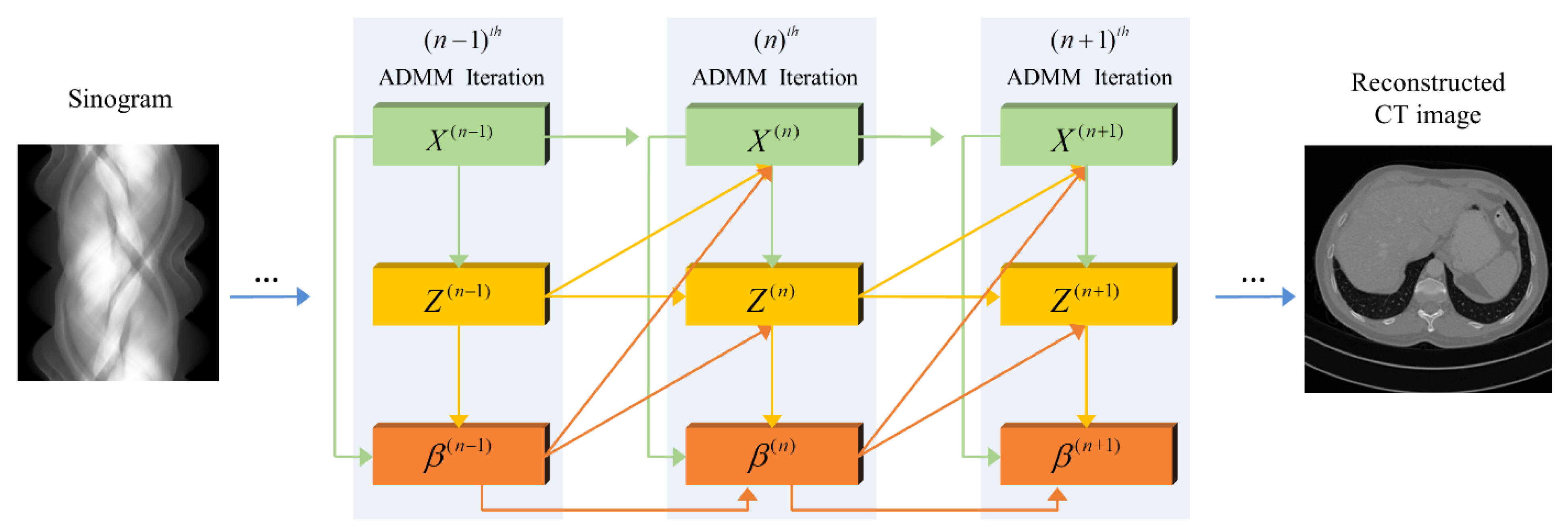
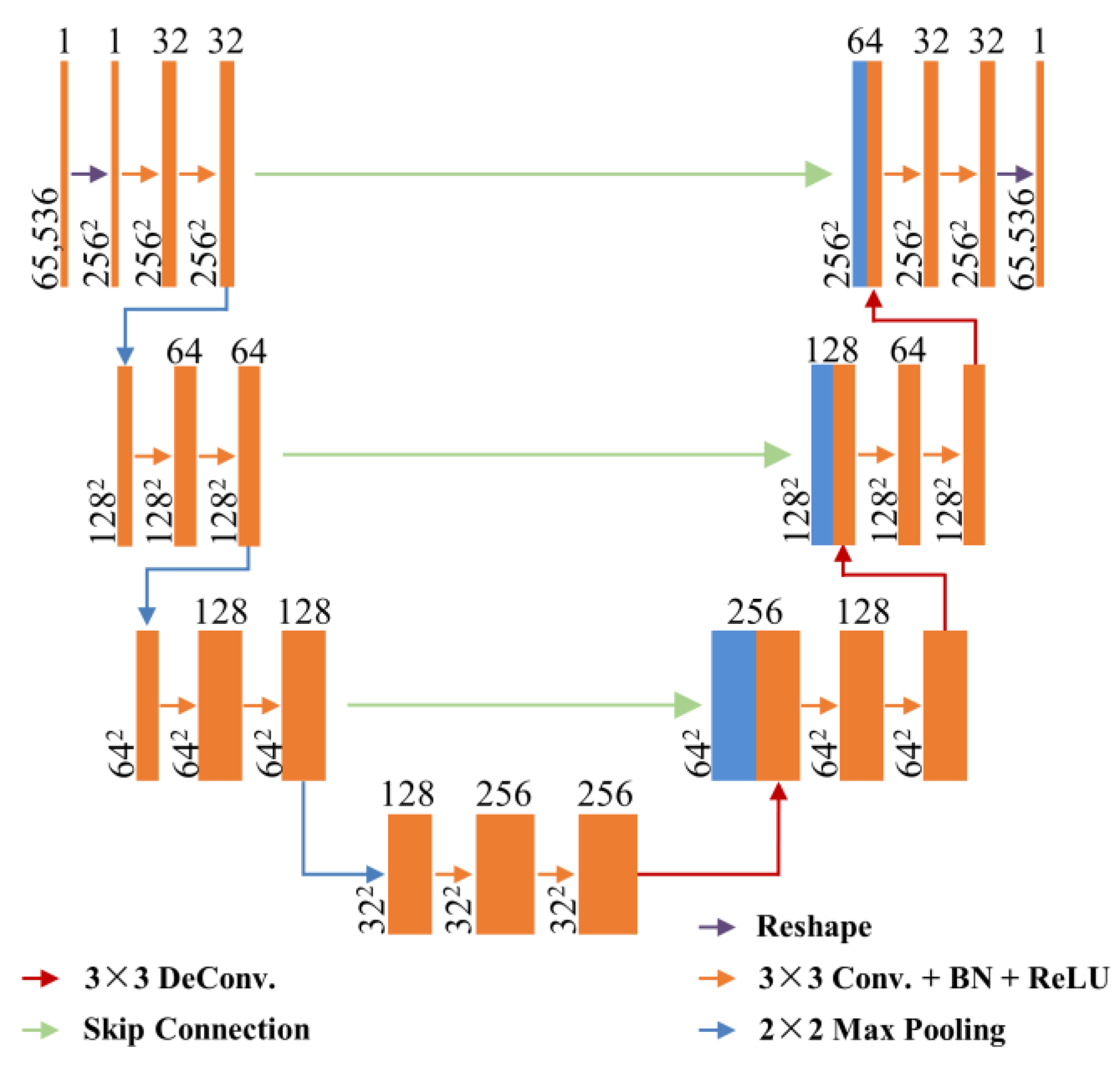
2.3. Proposed ADMM-Based Network

To solve the optimization problem with the ADMM algorithm as expressed in Equation (8), several parameters (i.e., {η, ρ, φ, γ}) need to be manually selected, and the sparse transformation of TV-based methods should be explicitly handcrafted and cannot be used for all kinds of images in different applications [31]. Therefore, in this paper, we propose an ADMM-based network to optimize the sparse transformation and the parameters in order to reconstruct high-quality CT images. The proposed network is shown in Figure 1.

We unified the parameters in Equation (8) in order to simplify the iteration process. The product of the two parameters was simplified to one parameter, which is convenient when training the network and improves the reconstruction efficiency. Specifically, θ = η ρ, ψ = φ ρ, and φ = φ λ. After these modifications, Equation (8) can be summarized as follows:

$$\{\begin{array}{l}{x}^{(n)}=x^{(n-1)}-\theta D^T(D{x}^{(n-1)}+{\beta }^{(n-1)}-z^{(n-1)})-\eta A^T(A{x}^{(n-1)}-y) \\ z^{(n)}=z^{(n-1)}+\psi (D{x}^{(n)}+{\beta }^{(n-1)}-z^{(n-1)})-\phi \mathrm{sgn}(z^{(n-1)} ) \\ {\beta }^{(n)}={\beta }^{(n-1)}+\gamma (D{x}^{(n)}-z^{(n)})\end{array}$$

(9)

The proposed method uses two modified U-net networks to replace D and D^T. Specifically, we used two sets of U-Net networks with the same structure but different random initial values to replace D and D^T. The gradient operator in the traditional TV-based reconstruction algorithm cannot express the edge and texture details well. In addition to the TV-based method, other methods can be used to represent the image sparse transformation, such as the dictionary [41] and wavelet-based [42] sparse representation methods. For images with different characteristics, different sparse transforms need to be manually selected. CNN-based networks give an outstanding performance in various imaging problems [43]. CNNs are capable of learning multiscale image features from large datasets with a cascade of simple modules. Among these CNN methods, because of the encoding and decoding structure with skip connections, the U-net [44] is capable of extracting more features from different layers.

To this end, a modified U-net network was used to represent the sparse transformation in this study. The architecture of the proposed modified U-net network is shown in Figure 2. The operators D and D^T in Equation (9) are regarded as two U-net architectures. Through training, the network learns the sparse transformation and all parameters adaptively.

As shown in Figure 2, the modified U-net consists of a reshaping operation, a convolution layer, a batch normalization layer, a rectified linear unit (ReLU), a max pooling layer, a deconvolution layer, and a skip connection layer. We made two changes to the U-net’s architecture. First, to control the scale of the network, we reduced the depth of the network and made the structure relatively compact, thus making the network more suitable for processing images that are 256 × 256 pixels in size. Second, to better connect the sparse transformation with other operations, we added reshaping operations to our network’s input and output. Since the other operations in Equation (9) are all for vectors, the convolution layer is an operation on images.

The proposed network needs to optimize the operators D and D^T (i.e., the parameters of the U-net architecture, denoted by Θ_D) and the parameter set {η, ψ, φ, γ} (denoted by Θ_P). All parameters Θ = {Θ_D} ∪ {Θ_P} are optimized by minimizing the loss function’s mean squared error (MSE):

$$E(\Theta )=\frac{1}{N}{\displaystyle \sum _{i=1}^N{\Vert x_i(\Theta )-x_i{}^{gt}\Vert }_2^2}$$

(10)

where x^gt is the corresponding ground truth image and N is the number of image pairs used to train the network.

3. Experimental Steps

3.1. Training Details

In our network, we optimized the loss function using the Adam algorithm [45]. During the training of the network, we initialized the parameters Θ_D = {filter size = 3 × 3, number of filters = 32}, and set the initial values of the parameter set Θ_P = {η = 2⁻⁵, ψ = 2⁻⁷, φ = 2⁻⁷, γ = −10⁻⁵}. Compared with Θ_D, the order of magnitude of Θ_P is quite small, so there is an imbalance in the process of training the network. Therefore, to fully train the network on Θ_D and Θ_P, we set different learning rates for these parameter sets. In the training process, if the validation loss remained unchanged for five epochs, the learning rate was reduced by a factor of 2. Specifically, the initial learning rate of Θ_D was set to 10⁻⁴ and slowly decreased to 3 × 10⁻⁶. The learning rate of Θ_P was set to 10⁻⁸ and slowly decreased to 3 × 10⁻¹⁰. The mini-batch size was set to 5. The number of ADMM iterations (stages) was set to 20. The initial input x⁽⁰⁾ was set to 0. Our network was trained using TensorFlow 2.2 and an Nvidia Titan RTX graphics card.

We selected three metrics to evaluate the reconstruction quality, namely the root mean square error (RMSE), the peak signal-to-noise ratio (PSNR), and the structural similarity index measure (SSIM) [46].

3.2. Dataset

To evaluate the network’s performance, we used open-access datasets authorized by the Mayo Clinic from “the 2016 NIH–AAPM–Mayo Clinic Low-Dose CT Grand Challenge” [47]. These datasets contain 5936 CT images from 10 patients with a resolution of 512 × 512, and the pixel size is 1 mm². The original projection data could not be directly used for the fan-beam CT image reconstruction because they were collected using a helix trajectory. As shown in

Table 1. Data acquisition parameters.

	Parameters	Value
1	Distance from the X-ray source to the detector arrays	1320.5 mm
2	Distance from the X-ray source to the center of rotation	1050.5 mm
3	Number of detectors	512
4	Detector pixel size	0.127 mm
5	Reconstruction size	256 × 256
6	Pixel size	1 mm2

, the sparse-view projections in our experiments were simulated from NDCT images that were downsampled to a size of 256 × 256 pixels. We performed forward projections of fan-beam scanning from the NDCT images for 32-, 64-, and 128-degree views. The distance from the X-ray source to the detector arrays was 1320.5 mm, the distance from the X-ray source to the center of rotation was 1050.5 mm, and we used 512 linear detectors with a bin size of 0.127 mm.

The reference images were the 100 KV NDCT scans reconstructed with a thickness of 1 mm and downsampled to a size of 256 × 256. The images of eight patients were used for training, and the images of the other two patients were used for verification and testing. In total, 3360 data pairs were used, in which 2240 data pairs were selected for training, and the remaining 1120 data pairs were used for verification and testing.

3.3. Comparison Methods

We compared our network against six reconstruction algorithms, including FBP [48], ART [8], ART-TV [22], TVAL3 [49], FBPConvNet [15], and LEARN [31]. The FBP algorithm is the most widely used analytic reconstruction algorithm, while ART is the most-used classic iterative algorithm for sparse-view reconstruction. ART-TV is an improvement on the ART algorithm that introduces image sparsity as prior information. The TVAL3 algorithm uses the ADMM algorithm to solve the constrained TV minimization CT model and was shown to have a better convergence speed and reconstruction effect than the other methods. The parameter μ was set to 2¹⁰, and the parameter β was set to 2⁷. In addition, we also chose two state-of-the-art deep-learning-based methods. FBPConvNet is a sparse-view CT postprocessing method based on a CNN. LEARN is a reconstruction algorithm based on a CNN, and its reconstruction effect is the best of all the methods. To make a fair comparison, the deep-learning-based methods were all trained the same dataset. The parameters were selected through experimentation to produce the best performance. Specifically, for the LEARN method, the number of filters was set to 48, the kernel size was set to 5, the number of iterations was set to 50, and the initial input to the network was set to 0. The initial learning rate was set to 10⁻⁴ and slowly decreased to 10⁻⁶. For the FBPConvNet method, the kernel size was set to 3, the initial learning rate was set to 10⁻⁴ and slowly decreased to 10⁻⁶, and the initial input to the network was set to the FBP result.

3.4. Robustness Validation

To verify the robustness of the proposed network to noise, we added different levels of Poisson noise to the test set for the 32-degree data. The noise was added according to the following formula [50]:

$$b_i=Poisson\left\{I_0{e}^{-y_i}\right\}$$

(11)

where b_i is the detector measurement along the ith ray, I₀ is the blank scan factor, and y_i is the line integral of the attenuation coefficients along the ith ray. In our experiment, the blank scan factor I₀ was set from 1 × 10⁷ to 1 × 10⁵.

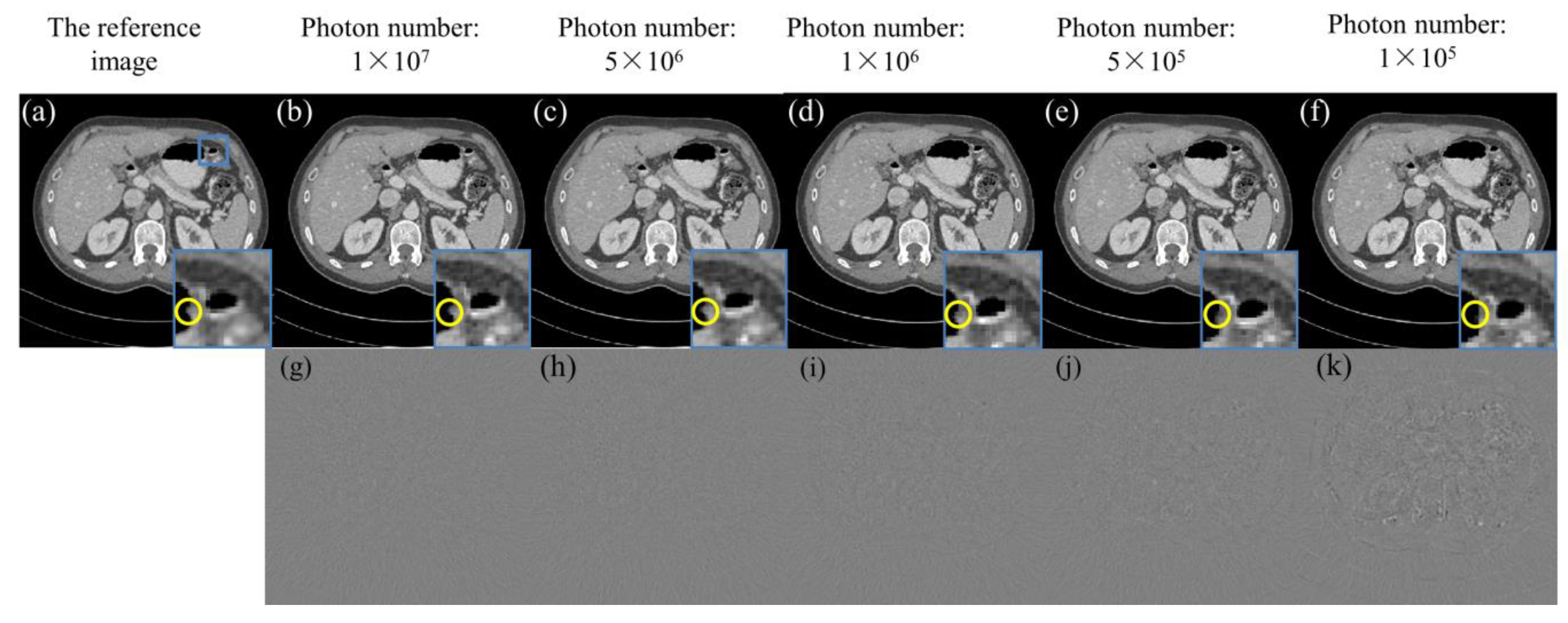
3.5. Low-Dose Reconstruction

To further verify the universality of the algorithm, we extended the sparse-view CT reconstruction task to a low-dose reconstruction task. We simulated low-dose projection data from their normal-dose counterparts as performed in 3pADMM [37]. Noise was added to the normal-dose sinogram as follows (I₀ = 5 × 10⁴, σ_e² = 10, approximately corresponding to the noise level acquired with a 20 mAs tube current):

$$nois{e}_i=Poisson\left\{I_0{e}^{-y_i}\right\}+Normal(0,{\sigma }_e{}^2)$$

(12)

where σ_e² is the variance in the electronic background noise. To evaluate the performance of our network under a low-dose CT projection, we chose 3pADMM for comparison. For a fair comparison, we trained our network on the same training dataset as that used by 3pADMM. The total number of training samples was 2378 data pairs, which is consistent with [37].

4. Results

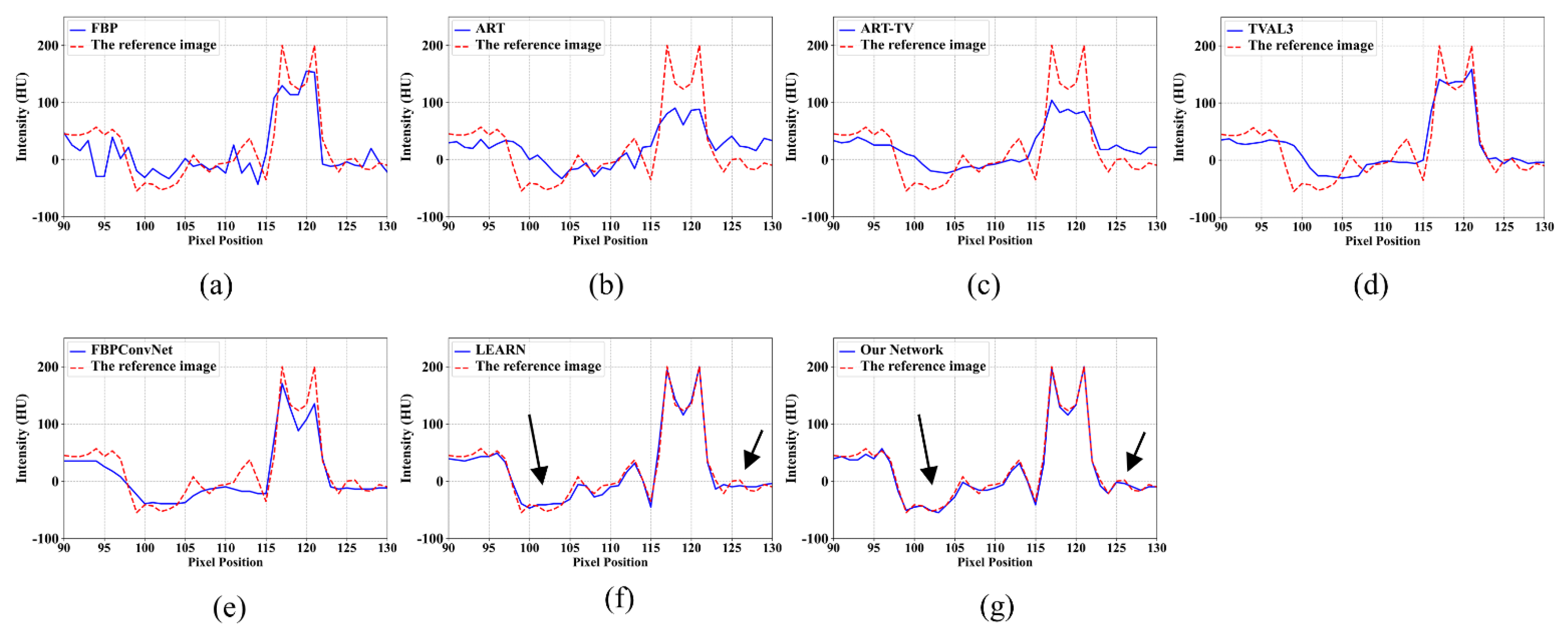
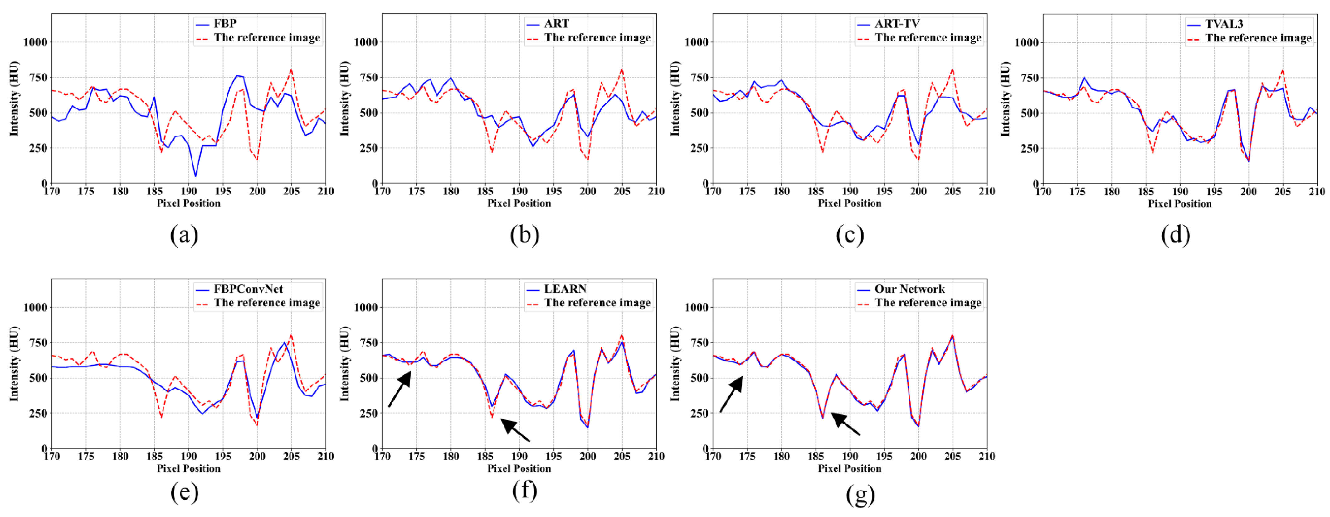
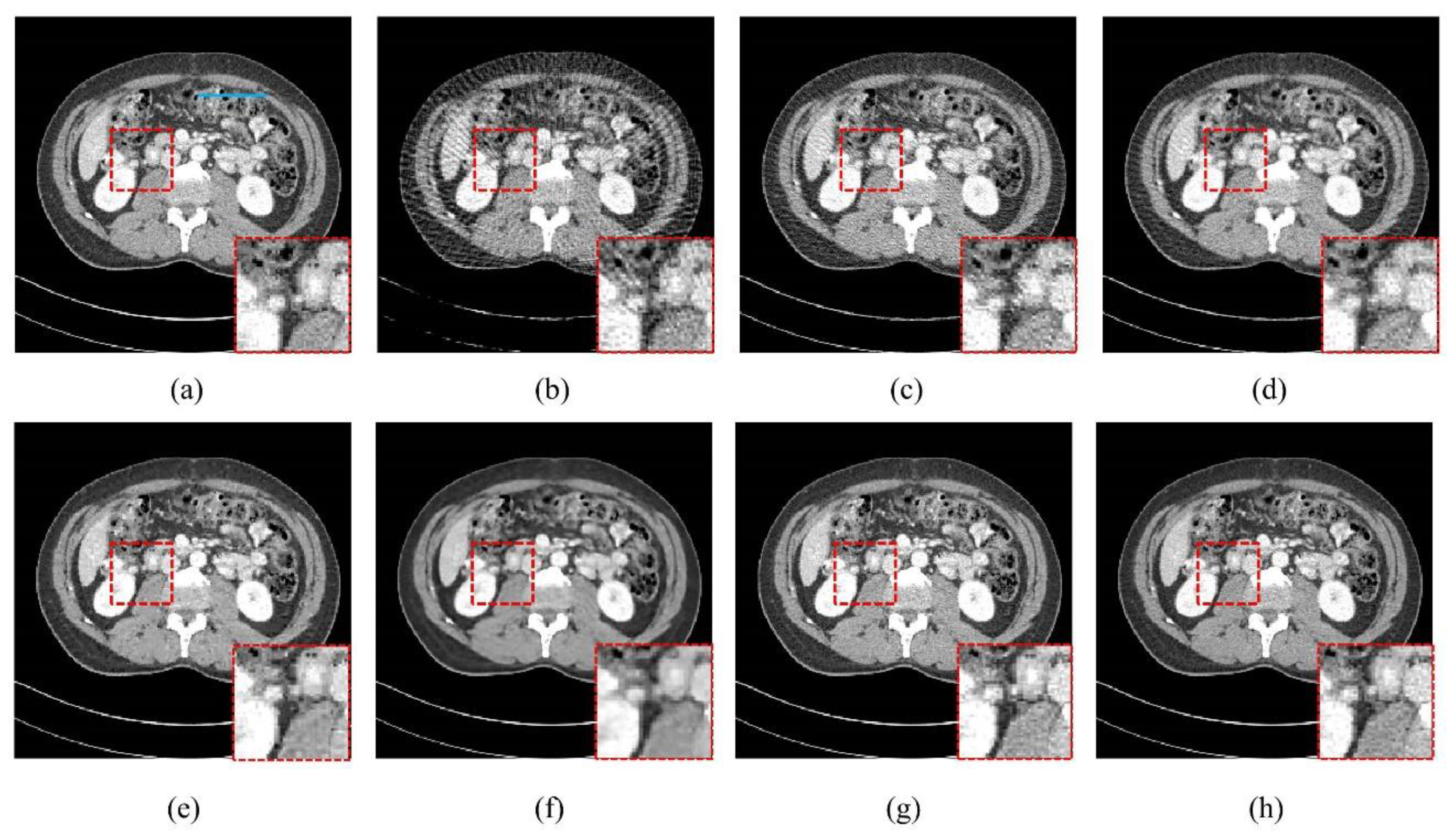
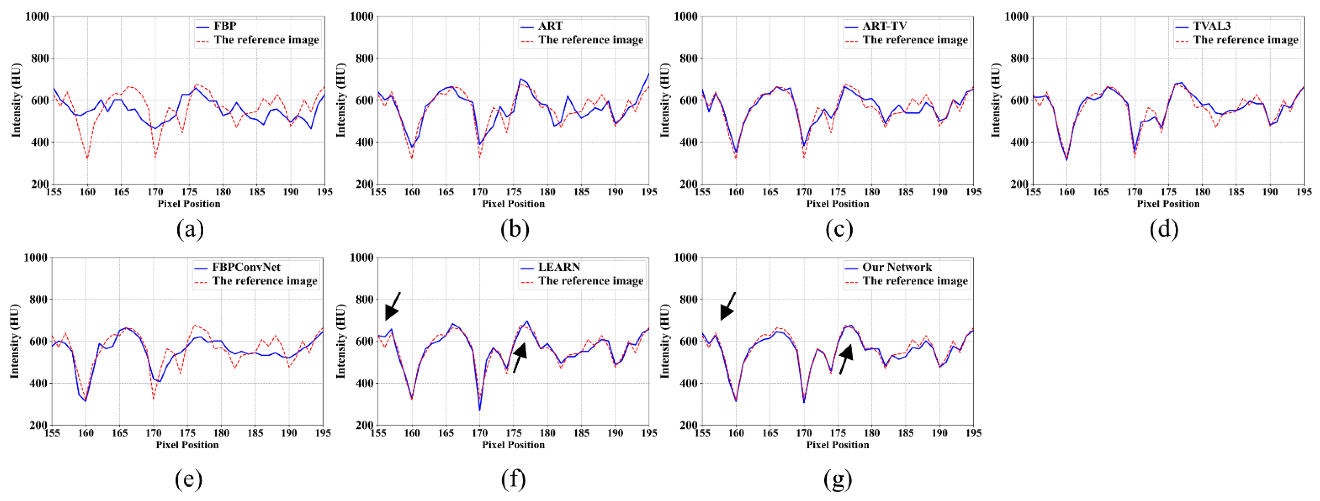
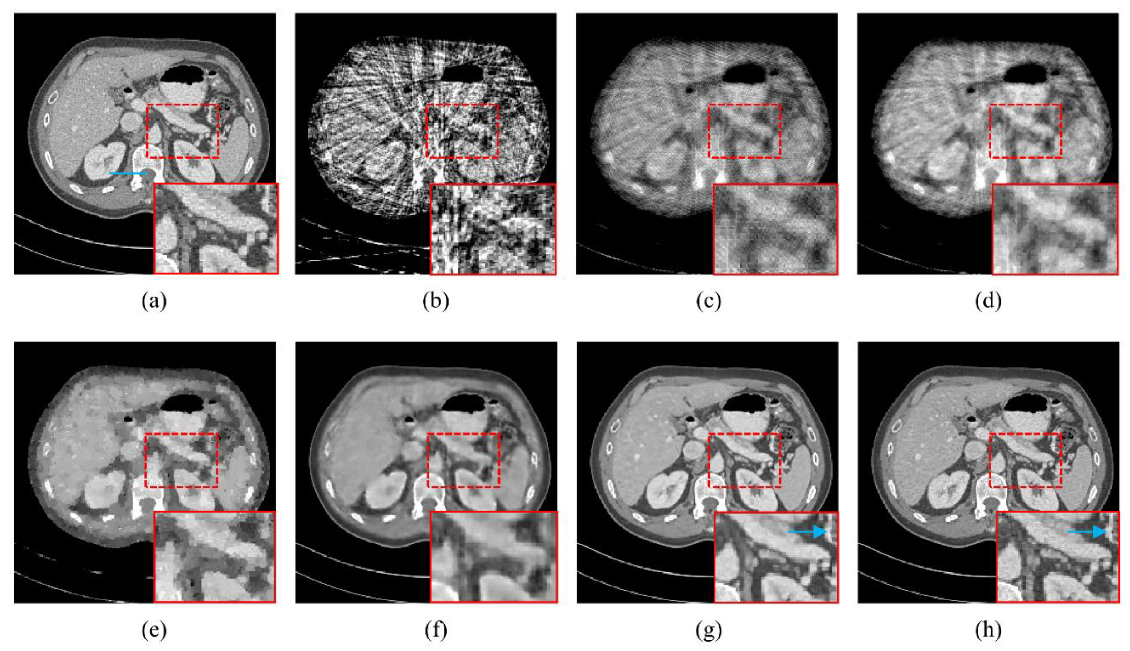
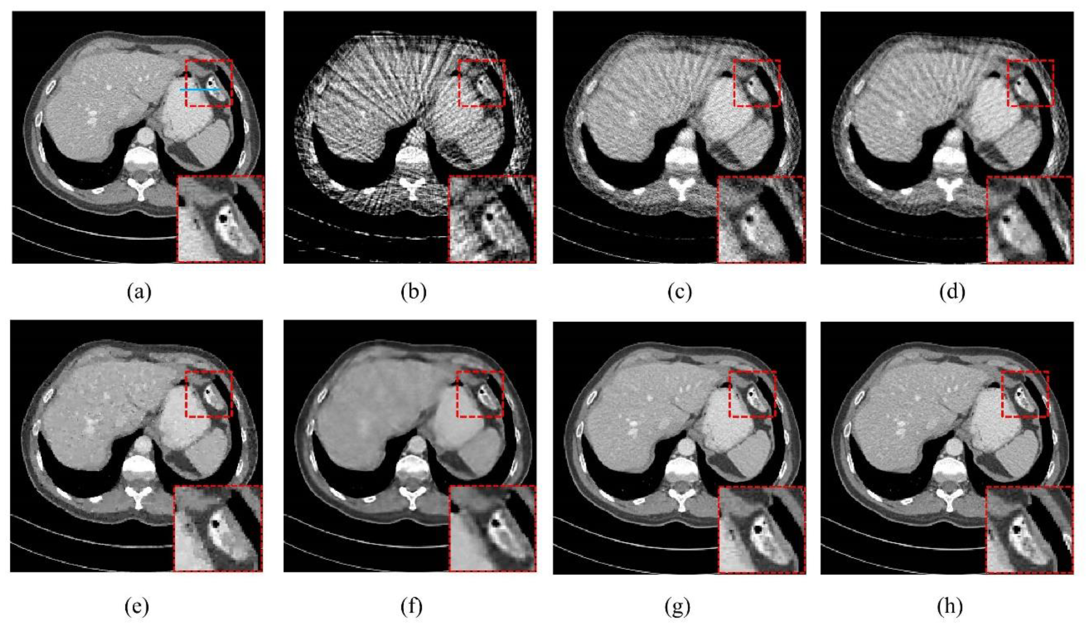
4.1. Visualization-Based Evaluation

To verify the performance of our network, we evaluated the network on the test dataset. Figure 3 shows the images that were reconstructed from 32 views using different methods. Since the projection is extremely sparse, the traditional reconstruction algorithms have difficulty obtaining detailed information as shown in Figure 3b–e. The result of the FBP algorithm has very serious streak artifacts. The results of the ART and ART-TV algorithms also have streak artifacts, and the reconstructed images are very blurry. The TVAL3 method suppresses the artifacts but the result is too vague to show details. The deep learning methods all achieve better results as shown in Figure 3f–h. The FBPConvNet method suppresses the streak artifacts, and the edges of most organs can be seen but they are blurry. However, many important details are smoothed out. In Figure 3g, the structure in the reconstruction results of the LEARN algorithm is complete and clear, and most of the details have been preserved. Although the LEARN algorithm reconstructed the structure, the details remain very blurry. The boundary of the image reconstructed by our method is clearer than that reconstructed by the LEARN algorithm. In addition, the black dots marked by the blue arrows were only reconstructed by our method. Figure 3h shows that our network obtained the best results as it presents the most details and the least difference from the reference image. To further demonstrate the ability of our method to preserve the structure, the horizontal profiles are shown in Figure 4. It is clear that our method is the most consistent with the reference image. The differences between our network and the LEARN method are marked by black arrows.

Figure 5 and Figure 6 show the reconstruction results and the horizontal profiles from 64 views, respectively. The reconstruction results significantly improve as the viewing angle increases. The reconstruction results obtained by the FBP, ART, and ART-TV algorithms still have noticeable streak artifacts. The result of the FBP algorithm has severe streak artifacts, while the results of the ART and ART-TV algorithms have relatively few streak artifacts. The TVAL3 algorithm eliminates most of the artifacts and provides more detailed information. The FBPConvNet algorithm still fails to reconstruct the small details with a lower contrast. The images obtained by the LEARN network and our algorithm have been well reconstructed, most of the details can be seen, and the regions with low contrast have been reconstructed very well. To better compare the differences between the two algorithms, the gray curve shown in Figure 6 shows that the image reconstructed by our network is closer to the ground truth image and more comprehensively displays the details.

For the reconstruction results from 128 views, the results of each algorithm have been significantly improved as shown in Figure 7. Only the result of the FBP method contains some obvious artifacts. The results of the ART and ART-TV algorithms still contain a small number of streak artifacts. The TVAL3 method eliminates most of the artifacts, and only some of the details have been smoothed out. The FBPConvNet algorithm overly smoothened the region in the middle of the image, and subtle details cannot be reliably obtained. The differences between the LEARN network and our network are barely discernible to the naked eye, and both networks have well reproduced the details in the image. The gray curve in Figure 8 shows that our algorithm is the most consistent with the gray curve of the reference image and that the reconstruction results are better than those of the other algorithms, demonstrating the capacity of our network to preserve the structure.

4.2. Quantitative and Qualitative Evaluation

Table 2. Quantitative results obtained for different methods.

Views	Index	FBP	ART	ART-TV	TVAL3	FBPConvNet	LEARN	Our Network
32	RMSE	0.11 5	0.04 9	0.046	0.033	0.03 4	0.01 8	0.009
	PSNR	19.013	26.267	26.685	29.547	29.479	39.209	40.839
	SSIM	0.57 8	0.789	0.817	0.90 8	0.90 3	0.91 2	0.96 7
64	RMSE	0.07 5	0.034	0.03 2	0.01 6	0.020	0.0 10	0.00 8
	PSNR	22.553	29.323	30.032	36.141	33.891	42.170	44.521
	SSIM	0.630	0.87 5	0.89 8	0.959	0.935	0.9 70	0.98 8
128	RMSE	0.049	0.01 7	0.01 4	0.008	0.010	0.00 7	0.006
	PSNR	26.141	35.675	37.098	41.670	39.824	45.131	46.085
	SSIM	0.826	0.955	0.96 9	0.970	0.951	0.977	0.99 5

presents the average quantitative results from 32, 64, and 128 views. In general, a smaller RMSE value represents a better reconstruction result, and the larger the PSNR and SSIM values, the more similar the reconstruction result is to the reference image. Compared with the LEARN algorithm, at 32, 64, and 128 views, our network achieves improvements in the RMSE of 0.009, 0.002, and 0.001, respectively. In addition, the PSNR index increases by 1.630, 2.351, and 0.954 and the SSIM increases by 0.055, 0.018, and 0.018, respectively. It can be seen that the values of the three metrics used to evaluate our network are better than those of the other algorithms. This result is consistent with the results of the visual assessment.

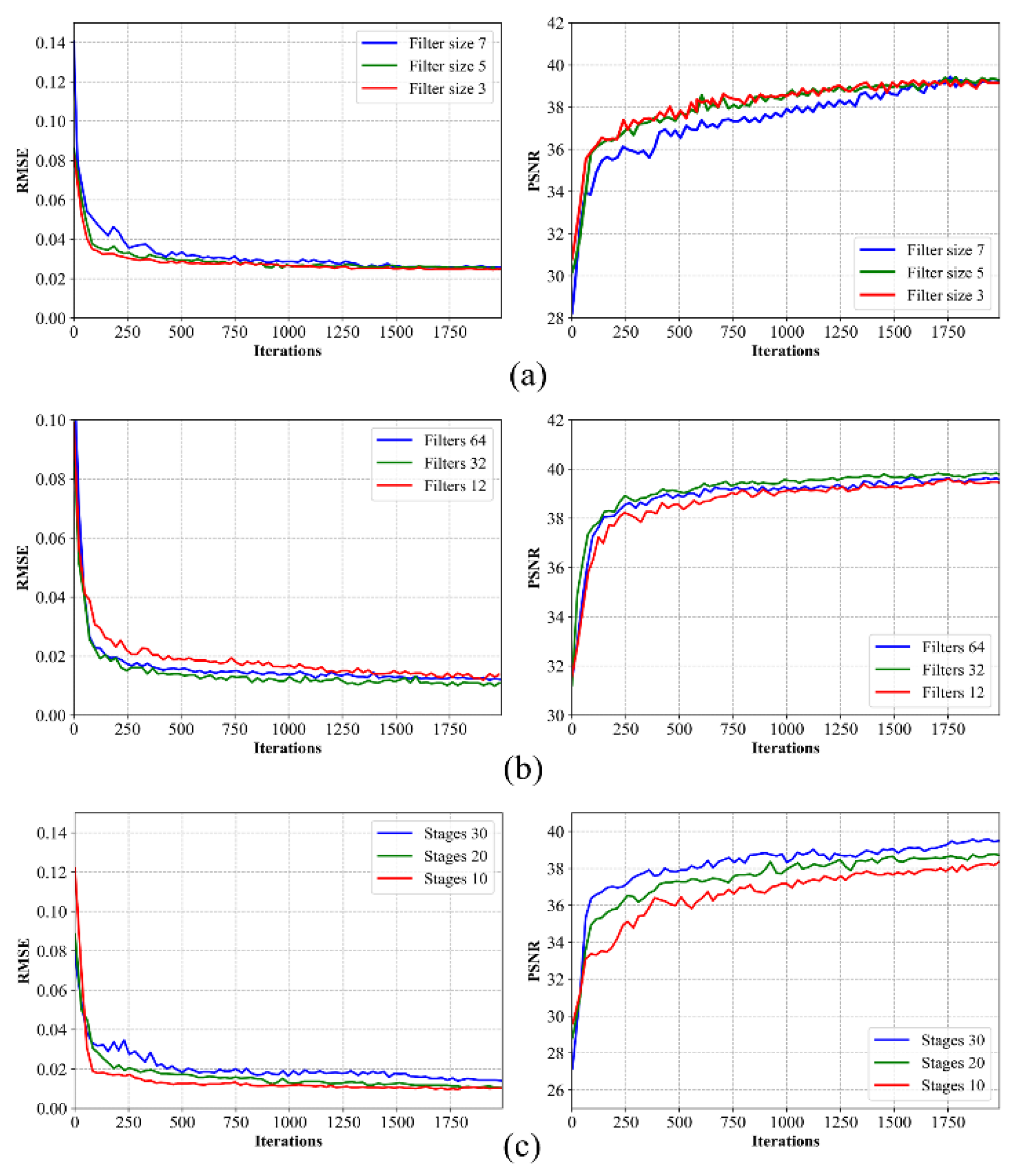
4.3. Model Structure Selection

Furthermore, we evaluated the impacts of several parameters of the network, including the number of filters, the filter size, and the number of ADMM iterations (stages), on the RMSE and PSNR. In this study, in all of the experiments, after optimizing the model on the corresponding 32-view training dataset, the performance was evaluated on the 32-view test set. The corresponding results are shown in Figure 9.

(1)

Impact of the Filter Size

We set the filter sizes to 3 × 3, 5 × 5, and 7 × 7, respectively, for testing. It can be seen that the performance did not obviously improve as the filter size increased, but when the filter size increased to 7, the values of the metrics began to decline, especially for PSNR. Based on these results, we set the filter size of the network to 3 × 3.

(2)

Number of Filters

We tested the cases where the number of filters was 64, 32, and 12, respectively. It can be seen that the performance improved as the number of filters increased, but the performance declined when the number of filters increased to 64. Based on these results, to balance the reconstruction performance and the computing cost, the number of filters was finally set to 32 in our network.

(3)

Number of Stages

Finally, we evaluated the impact of the number of ADMM iterations (stages) on the performance of the network. We set the number of stages to 10, 20, and 30. It can be seen that the PSNR improved and the RMSE decreased as the number of stages increased. The RMSE became worse mainly because the larger number of iterations increased the computational burden on the network training, resulting in a slower decline in the RMSE. In addition, the number of stages is proportional to the reconstruction time. Based on these results, to balance the reconstruction performance and the time cost, the number of ADMM iterations was finally set to 20 in our network.

4.4. Robustness Results

Figure 10 presents the results of our network for different noise levels and the absolute residuals between the reconstructed image and the reference image at different noise levels.

Table 3. Robustness analysis results for different noise levels.

Photon Number	1 × 105	5 × 105	1 × 106	5 × 106	1 × 107
RMSE	0.0111	0.0089	0.0085	0.0083	0.0081
PSNR	39.0873	41.0521	41.4174	41.6286	41.7647
SSIM	0.9787	0.9850	0.9860	0.9867	0.9869

shows the test results on the RMSE, PSNR, and SSIM at different noise levels. As shown in Figure 10, the performance of our network is quite stable and it can effectively suppress noise. When I₀ is greater than 5 × 10⁵, our network can effectively eliminate noise. When the noise level was higher than 1 × 10⁵, the performance of our network began to gradually deteriorate. These experimental results show that our network can deal with a wide range of noise levels.

4.5. Low-Dose Reconstruction Results

Table 4. Low-dose reconstruction results for different algorithms.

Methods	NMSE	PSNR	FSIM
3pADMM(40)	0.018	39.242	0.948
Our Network	0.017	40.139	0.949

shows the low-dose reconstruction results of the normalized mean-square error (NMSE), PSNR, and feature similarity (FSIM) [51]. Compared with the results in [37], our results show more advantages in the NMSE, PSNR, and FSIM. It can be seen that our network performs well in low-dose reconstruction tasks and has better performance than the 3pADMM algorithm.

5. Discussion and Conclusions

In this paper, we studied the sparse-view CT reconstruction of medical images. Focusing on the difficulties with the use of traditional model-driven imaging methods, we carried out research on data-driven CT reconstruction methods. In this study, in order to overcome the difficulty with choosing prior information and parameters in the model-driven reconstruction method, an efficient reconstruction network based on the ADMM for sparse-view CT images is proposed. The ADMM algorithm was expanded into a deep learning framework, and the sparse transform of the image was represented by a modified U-net. The model parameters and the sparse transformation were simultaneously optimized in the iterative framework. Compared with recent state-of-the-art reconstruction algorithms, our proposed network showed superior performance in a visualization-based evaluation and in terms of various evaluation metrics. Experiments were carried out under the condition of increasing Poisson noise, and the robustness to noise was verified. Both the qualitative and quantitative results indicate the effectiveness of our method for sparse-view CT image reconstruction. Furthermore, we extended the sparse-view CT image reconstruction task to a low-dose reconstruction task in order to verify the universality of our algorithm.

There are three main reasons for the promising performance of our reconstruction method. First, we used the superior performance of the ADMM algorithm to optimize the model. In cases of extremely sparse views (such as 32 views), our algorithm has more obvious advantages than the other algorithms, and the intricate details are almost completely retained. Second, by decomposing the formula, we trained a modified U-net to obtain the sparse transformation and took full advantage of the capability of the U-net for feature extraction. Finally, during the training process, the parameters of both the ADMM algorithm and the modified U-net were simultaneously optimized, making these methods more adaptive to the data.

However, there are some limitations to our approach. Due to the computing costs, our network can only reconstruct images with a size of 256 × 256 pixels. In future work, we will continue to optimize the model so that it can be applied to higher-resolution images. We will consider the use of parallel acceleration on multi-GPU platforms to address data and memory issues. In addition, the research presented in this paper was aimed at the two-dimensional situation, so future research could generalize the algorithm to the three-dimensional situation. Future research could also extend our network to other optimization problems of multiple separable objective functions, such as image decomposition and image denoising.

References

1. Hounsfield, G.N. Computerized transverse axial scanning (tomography): Part 1. Description of system. Br. J. Radiol. 1973, 46, 1016–1022. [Google Scholar] [CrossRef] [PubMed]
2. Wang, G.; Yu, H.; De Man, B. An outlook on x-ray CT research and development. Med. Phys. 2008, 35, 1051–1064. [Google Scholar] [CrossRef] [PubMed] [Green Version]
3. Slovis, T.L. The ALARA concept in pediatric CT: Myth or reality? Radiology 2002, 223, 5–6. [Google Scholar] [CrossRef]
4. Chen, Y.; Shi, L.; Feng, Q.; Yang, J.; Shu, H.; Luo, L.; Coatrieux, J.; Chen, W. Artifact Suppressed Dictionary Learning for Low-Dose CT Image Processing. IEEE Trans. Med. Imaging 2014, 33, 2271–2292. [Google Scholar] [CrossRef] [PubMed]
5. Chen, G.-H.; Tang, J.; Leng, S. Prior image constrained compressed sensing (PICCS): A method to accurately reconstruct dynamic CT images from highly undersampled projection data sets. Med. Phys. 2008, 35, 660–663. [Google Scholar] [CrossRef] [PubMed] [Green Version]
6. Li, H.; Li, J.; Lin, X.; Qian, X. A Model-Driven Stack-Based Fully Convolutional Network for Pancreas Segmentation. In Proceedings of the 2020 5th International Conference on Communication, Image and Signal Processing, CCISP 2020, Chengdu, China, 13–15 November 2020. [Google Scholar]
7. Chetih, N.; Messali, Z. Tomographic image reconstruction using filtered back projection (FBP) and algebraic reconstruction technique (ART). In Proceedings of the 3rd International Conference on Control, Engineering and Information Technology, CEIT 2015, Tlemcen, Algeria, 25–27 May 2015. [Google Scholar]
8. Gordon, R.; Bender, R.; Herman, G.T. Algebraic Reconstruction Techniques (ART) for three-dimensional electron microscopy and X-ray photography. J. Theor. Biol. 1970, 29, 471–481. [Google Scholar] [CrossRef]
9. Andersen, A.H.; Kak, A.C. Simultaneous Algebraic Reconstruction Technique (SART): A superior implementation of the ART algorithm. Ultrason. Imaging 1984, 6, 81–94. [Google Scholar] [CrossRef] [PubMed]
10. Moon, T.K. The expectation-maximization algorithm. IEEE Signal Process. Mag. 1996, 13, 47–60. [Google Scholar] [CrossRef]
11. Chakradar, M.; Aggarwal, A.; Cheng, X.; Rani, A.; Kumar, M.; Shankar, A. A Non-invasive Approach to Identify Insulin Resistance with Triglycerides and HDL-c Ratio Using Machine learning. Neural Process. Lett. 2021, 2, 1–21. [Google Scholar] [CrossRef]
12. Goyal, V.; Singh, G.; Tiwari, O.M.; Punia, S.K.; Kumar, M. Intelligent skin cancer detection mobile application using convolution neural network. J. Adv. Res. Dyn. Control Syst. 2019, 11, 253–259. [Google Scholar]
13. Boublil, D.; Elad, M.; Shtok, J.; Zibulevsky, M. Spatially-Adaptive Reconstruction in Computed Tomography Using Neural Networks. IEEE Trans. Med. Imaging 2015, 34, 1474–1485. [Google Scholar] [CrossRef] [PubMed] [Green Version]
14. Wolterink, J.M.; Leiner, T.; Viergever, M.A.; Išgum, I. Generative adversarial networks for noise reduction in low-dose CT. IEEE Trans. Med. Imaging 2017, 36, 2536–2545. [Google Scholar] [CrossRef] [PubMed]
15. Jin, K.H.; McCann, M.T.; Froustey, E.; Unser, M. Deep Convolutional Neural Network for Inverse Problems in Imaging. IEEE Trans. Image Process. 2017, 26, 4509–4522. [Google Scholar] [CrossRef] [PubMed] [Green Version]
16. Chen, H.; Zhang, Y.; Kalra, M.K.; Lin, F.; Chen, Y.; Liao, P.; Zhou, J.; Wang, G. Low-Dose CT With a Residual Encoder-Decoder Convolutional Neural Network. IEEE Trans. Med. Imaging 2017, 36, 2524–2535. [Google Scholar] [CrossRef]
17. Zhang, Z.; Liang, X.; Dong, X.; Xie, Y.; Cao, G. A Sparse-View CT Reconstruction Method Based on Combination of DenseNet and Deconvolution. IEEE Trans. Med. Imaging 2018, 37, 1407–1417. [Google Scholar] [CrossRef]
18. Kang, E.; Min, J.; Ye, J.C. A deep convolutional neural network using directional wavelets for low-dose X-ray CT reconstruction. Med. Phys. 2017, 44, 330–375. [Google Scholar] [CrossRef] [Green Version]
19. Yang, Q.; Yan, P.; Zhang, Y.; Yu, H.; Shi, Y.; Mou, X.; Kalra, M.K.; Zhang, Y.; Sun, L.; Wang, G. Low-Dose CT Image Denoising Using a Generative Adversarial Network With Wasserstein Distance and Perceptual Loss. IEEE Trans. Med. Imaging 2018, 37, 1348–1357. [Google Scholar] [CrossRef]
20. Zhang, H.; Liu, B.; Yu, H.; Dong, B. MetaInv-Net: Meta Inversion Network for Sparse View CT Image Reconstruction. IEEE Trans. Med. Imaging 2021, 40, 621–634. [Google Scholar] [CrossRef]
21. Donoho, D.L. Compressed sensing. IEEE Trans. Inf. Theory 2006, 52, 1289–1306. [Google Scholar] [CrossRef]
22. LaRoque, S.J.; Sidky, E.Y.; Pan, X. Accurate image reconstruction from few-view and limited-angle data in diffraction tomography. J. Opt. Soc. Am. A. Opt. Image Sci. Vis. 2008, 25, 1772–1782. [Google Scholar] [CrossRef] [Green Version]
23. Sidky, E.Y.; Pan, X. Image reconstruction in circular cone-beam computed tomography by constrained, total-variation minimization. Phys. Med. Biol. 2008, 53, 4777–4807. [Google Scholar] [CrossRef] [PubMed] [Green Version]
24. Rauhut, H.; Schnass, K.; Vandergheynst, P. Compressed Sensing and Redundant Dictionaries. IEEE Trans. Inf. Theory 2008, 54, 2210–2219. [Google Scholar] [CrossRef] [Green Version]
25. Chen, Y.; Ye, X.; Huang, F. A novel method and fast algorithm for MR image reconstruction with significantly under-sampled data. Inverse Probl. Imaging 2010, 4, 223–240. [Google Scholar] [CrossRef]
26. Xu, Q.; Yu, H.; Mou, X.; Zhang, L.; Hsieh, J.; Wang, G. Low-Dose X-ray CT Reconstruction via Dictionary Learning. IEEE Trans. Med. Imaging 2012, 31, 1682–1697. [Google Scholar] [CrossRef] [PubMed] [Green Version]
27. Würfl, T.; Hoffmann, M.; Christlein, V.; Breininger, K.; Huang, Y.; Unberath, M.; Maier, A.K. Deep Learning Computed Tomography: Learning Projection-Domain Weights From Image Domain in Limited Angle Problems. IEEE Trans. Med. Imaging 2018, 37, 1454–1463. [Google Scholar] [CrossRef] [PubMed]
28. Lee, H.; Lee, J.; Kim, H.; Cho, B.; Cho, S. Deep-Neural-Network-Based Sinogram Synthesis for Sparse-View CT Image Reconstruction. IEEE Trans. Radiat. Plasma Med. Sci. 2019, 3, 109–119. [Google Scholar] [CrossRef] [Green Version]
29. Zhou, B.; Zhou, S.K.; Duncan, J.S.; Liu, C. Limited View Tomographic Reconstruction using a Cascaded Residual Dense Spatial-Channel Attention Network with Projection Data Fidelity Layer. IEEE Trans. Med. Imaging 2021, 40, 1792–1804. [Google Scholar] [CrossRef] [PubMed]
30. Gupta, H.; Jin, K.H.; Nguyen, H.Q.; McCann, M.T.; Unser, M. CNN-Based Projected Gradient Descent for Consistent CT Image Reconstruction. IEEE Trans. Med. Imaging 2018, 37, 1440–1453. [Google Scholar] [CrossRef] [Green Version]
31. Chen, H.; Zhang, Y.; Chen, Y.; Zhang, J.; Zhang, W.; Sun, H.; Lv, Y.; Liao, P.; Zhou, J.; Wang, G. LEARN: Learned Experts’ Assessment-Based Reconstruction Network for Sparse-Data CT. IEEE Trans. Med. Imaging 2018, 37, 1333–1347. [Google Scholar] [CrossRef] [PubMed]
32. Boyd, S.; Parikh, N.; Chu, E.; Peleato, B.; Eckstein, J. Distributed Optimization and Statistical Learning via the Alternating Direction Method of Multipliers. Found. Trends® Mach. Learn. 2011, 3, 1–122. [Google Scholar] [CrossRef]
33. Xiao, Y.; Zhu, H.; Wu, S.-Y. Primal and dual alternating direction algorithms for ℓ1-ℓ1-norm minimization problems in compressive sensing. Comput. Optim. Appl. 2013, 54, 441–459. [Google Scholar] [CrossRef]
34. Yang, Y.; Sun, J.; Li, H.; Xu, Z. Deep ADMM-Net for compressive sensing MRI. Adv. Neural Inf. Process. Syst. 2016, 29, 10–18. [Google Scholar]
35. Yang, Y.; Sun, J.; Li, H.; Xu, Z. ADMM-CSNet: A Deep Learning Approach for Image Compressive Sensing. IEEE Trans. Pattern Anal. Mach. Intell. 2020, 42, 521–538. [Google Scholar] [CrossRef] [PubMed]
36. Li, Y.; Cheng, X.; Gui, G. Co-Robust-ADMM-Net: Joint ADMM Framework and DNN for Robust Sparse Composite Regularization. IEEE Access 2018, 6, 47943–47952. [Google Scholar] [CrossRef]
37. He, J.; Yang, Y.; Wang, Y.; Zeng, D.; Bian, Z.; Zhang, H.; Sun, J.; Xu, Z.; Ma, J. Optimizing a Parameterized Plug-and-Play ADMM for Iterative Low-Dose CT Reconstruction. IEEE Trans. Med. Imaging 2019, 38, 371–382. [Google Scholar] [CrossRef]
38. Zhang, H.; Dong, B.; Liu, B. JSR-Net: A Deep Network for Joint Spatial-radon Domain CT Reconstruction from Incomplete Data. In Proceedings of the ICASSP 2019—2019 IEEE International Conference on Acoustics, Speech and Signal Processing (ICASSP), Brighton, UK, 12–17 May 2019; pp. 3657–3661. [Google Scholar]
39. Wang, J.; Zeng, L.; Wang, C.; Guo, Y. ADMM-based deep reconstruction for limited-angle CT. Phys. Med. Biol. 2019, 64, 115011. [Google Scholar] [CrossRef]
40. Wang, G.; Ye, Y.; Yu, H. Approximate and Exact Cone-Beam Reconstruction with Standard and Non-Standard Spiral Scanning. Phys. Med. Biol. 2007, 52, 1–13. [Google Scholar] [CrossRef]
41. Li, S.; Cao, Q.; Chen, Y.; Hu, Y.; Luo, L.; Toumoulin, C. Dictionary learning based sinogram inpainting for CT sparse reconstruction. Optik 2014, 125, 2862–2867. [Google Scholar] [CrossRef] [Green Version]
42. Lee, M.; Kim, H.; Kim, H.J. Sparse-view CT reconstruction based on multi-level wavelet convolution neural network. Phys. Medica 2020, 80, 352–362. [Google Scholar] [CrossRef]
43. Schlemper, J.; Caballero, J.; Hajnal, J.V.; Price, A.N.; Rueckert, D. A Deep Cascade of Convolutional Neural Networks for Dynamic MR Image Reconstruction. IEEE Trans. Med. Imaging 2018, 37, 491–503. [Google Scholar] [CrossRef] [Green Version]
44. Ronneberger, O.; Fischer, P.; Brox, T. U-Net: Convolutional Networks for Biomedical Image Segmentation. In Medical Image Computing and Computer-Assisted Intervention—MICCAI 2015; Navab, N., Hornegger, J., Wells, W.M., Frangi, A.F., Eds.; Springer International Publishing: Cham, Switzerland, 2015; pp. 234–241. [Google Scholar]
45. Kingma, D.P.; Ba, J. Adam: A Method for Stochastic Optimization. In Proceedings of the 3rd International Conference on Learning Representations, ICLR 2015, San Diego, CA, USA, 7–9 May 2015. [Google Scholar]
46. Wang, Z.; Bovik, A.C.; Sheikh, H.R.; Simoncelli, E.P. Image quality assessment: From error visibility to structural similarity. IEEE Trans. Image Process. 2004, 13, 600–612. [Google Scholar] [CrossRef] [PubMed] [Green Version]
47. The 2016 NIH-AAPM-Mayo Clinic Low Dose CT Grand Challenge. Available online: http://www.aapm.org/GrandChallenge/LowDoseCT/ (accessed on 25 January 2022).
48. Kak, A.C.; Slaney, M. Principles of Computerized Tomographic Imaging; Classics in Applied Mathematics; SIAM: Philadelphia, PA, USA, 2001; Volume 33, ISBN 978-0-89871-494-4. [Google Scholar]
49. Chengbo, L.; Yin, W.; Zhang, Y. TVAL3: TV Minimization by Augmented Lagrangian and Alternating Direction Algorithms. Available online: https://www.caam.rice.edu/~optimization/L1/TVAL3/ (accessed on 25 January 2022).
50. Li, T.; Li, X.; Wang, J.; Wen, J.; Lu, H.; Hsieh, J.; Liang, Z. Nonlinear sinogram smoothing for low-dose X-ray CT. IEEE Trans. Nucl. Sci. 2004, 51, 2505–2513. [Google Scholar] [CrossRef]
51. Zhang, L.; Zhang, L.; Mou, X.; Zhang, D. FSIM: A feature similarity index for image quality assessment. IEEE Trans. Image Process. 2011, 20, 2378. [Google Scholar] [CrossRef] [PubMed] [Green Version]
Figure 1. The overall structure of our proposed network. The modules with the three different colors correspond to layer(X(n)), layer(Z(n)), and layer(β(n)). Each ADMM iteration of the network consists of these three types of layers.
Photonics 09 00186 g001
Figure 2. The structure of the proposed network, where the numbers in each layer indicate the shape of its output. Conv, convolution layer; DeConv, deconvolution layer; BN, batch normalization; ReLU, rectified linear unit.
Photonics 09 00186 g002
Figure 3. Images reconstructed (from 32 views) using various reconstruction methods. (a) The reference image versus the images reconstructed using (b) FBP, (c) ART, (d) ART-TV, (e) TVAL3, (f) FBPConvNet, (g) LEARN, and (h) our network. The profiles along the blue line are shown in Figure 4. The red box indicates the ROI, which is magnified. The display window is [−150, 250] HUs in size.
Photonics 09 00186 g003
Figure 4. Horizontal profiles along the blue line shown in Figure 3a of the reference image versus the images reconstructed (from 32 views) using (a) FBP, (b) ART, (c) ART-TV, (d) TVAL3, (e) FBPConvNet, (f) LEARN, and (g) our network. The differences between our network and the LEARN method are marked by black arrows.
Photonics 09 00186 g004
Figure 5. Images reconstructed (from 64 views) using various methods. (a) The reference image versus the images reconstructed using (b) FBP, (c) ART, (d) ART-TV, (e) TVAL3, (f) FBPConvNet, (g) LEARN, and (h) our network. The profiles along the blue line are shown in Figure 6. The red box indicates the ROI, which is magnified. The display window is [0, 1100] HUs in size.
Photonics 09 00186 g005
Figure 6. Horizontal profiles along the blue line shown in Figure 5a of the reference image versus the images reconstructed (from 64 views) using (a) FBP, (b) ART, (c) ART-TV, (d) TVAL3, (e) FBPConvNet, (f) LEARN, and (g) our network. The differences between our network and the LEARN network are marked by black arrows.
Photonics 09 00186 g006
Figure 7. Images reconstructed (from 128 views) using various methods. (a) The reference image versus the images reconstructed using (b) FBP, (c) ART, (d) ART-TV, (e) TVAL3, (f) FBPConvNet, (g) LEARN, and (h) our network. The profiles along the blue line are shown in Figure 8. The red box indicates the ROI, which is magnified. The display window is [200, 1000] HUs in size.
Photonics 09 00186 g007
Figure 8. Horizontal profiles along the blue line shown in Figure 7a of the reference image versus the images reconstructed (from 128 views) using (a) FBP, (b) ART, (c) ART-TV, (d) TVAL3, (e) FBPConvNet, (f) LEARN, and (g) our network. The differences between our network and the LEARN network are marked by black arrows.
Photonics 09 00186 g008
Figure 9. Model structure selection based on quantitative measures of the RMSE and PSNR as evaluated on the test dataset during training: (a) filter size; (b) number of filters; (c) number of stages.
Photonics 09 00186 g009
Figure 10. Reconstructed results (from 32 views) and absolute residuals at different noise levels. (a) The reference image, (b) our network result with I0 = 1 × 10⁷, (c) the result with I0 = 5 × 10⁶, (d) the result with I0 = 1 × 10⁶, (e) the result with I0 = 5 × 10⁵, and (f) the result with I0 = 1 × 10⁵. The display window is [−150, 250] HUs in size. (g) The residual error between (b) and (a), (h) the residual error between (c) and (a), (i) the residual error between (d) and (a), (j) the residual error between (e) and (a), and (k) the residual error between (f) and (a). The display window is [−0.2, 0.2].
Photonics 09 00186 g010