Improved Search Algorithm of Digital Speckle Pattern Based on PSO and IC-GN

Abstract

Digital speckle correlation method has not only been widely used in a variety of photometric mechanical scenarios, but also integrated with multiple disciplines. In the future, it will even be inextricably linked to the Internet of Things, autonomous driving, deep learning and other fields. For a given hardware condition, it is of great significance to improve the efficiency of integer-pixel search and increase the accuracy and efficiency of the sub-pixel algorithm. In this paper, we propose an improved digital speckle correlation method, which consists of an integer-pixel search algorithm and a sub-pixel search algorithm. With respect to the integer-pixel search, aiming to address the two problems of uniqueness of maximum value and parameter setting of PSO-W algorithm, the algorithm PSO-1 is proposed, and the results of comparison experiments show that it has higher search efficiency. In terms of sub-pixels, based on IC-GN algorithm with the highest accuracy at present, the IV-ICGN algorithm is proposed, and the simulation experiment results show that the proposed algorithm has higher accuracy and higher efficiency than the comparison algorithm.

1. Introduction

Digital image correlation method (DICM) uses the speckle images of an object before and after deformation to obtain the displacement information of the object by matching the positions of the most similar subsets of these scattered images according to the correlation function. Since there are no common objects (such as feature points, characteristic curves, specific pixel sets, etc.) in the obtained images, which is only composed of a large number of random speckles, thus it is also known as digital speckle correlation method (DSCM). Due to the advantages of non-destructive, non-contact, low cost and low requirements for the measurement environment, as well as the ability to provide high-resolution displacement and strain fields, DSCM has been widely used in scientific research and engineering practice, such as civil engineering [1,2], biology [3,4,5], medicine [6,7], aerospace [8,9,10], industrial manufacturing [11,12], material science [13,14,15], Internet of Things [16], autonomous driving technology [17], deep learning algorithm [18], nanotechnology [19] and X-ray CT scanning technique [20,21].

DSCM was proposed by Peters and Ranson [22] and applied to photogrammetry, which has been improved in the following 20 years by Peters [23], Chen [24], Schreier [25] and Wang [26]. DSCM has two very important research directions: to locate the initial position of a pixel through the integer-pixel displacement search and to obtain sub-pixel displacement value through sub-pixel displacement search.

In terms of integer-pixel displacement search, the commonly used algorithms are traditional algorithms such as point-by-point search method, cross search method [27], coarse and fine search method [28] and intelligent search algorithms based on artificial fish swarms algorithm (AFSA) [29], genetic algorithm (GA) [29], particle swarm optimization (PSO) [30], etc. Jiang et al. [31] proposed a cross-correlation algorithm based on fast Fourier transform, which improved the searching efficiency and robustness without sacrificing accuracy. Zhong et al. [32] used gradient orientation technology to improve the coarse search efficiency of integer-pixel search by more than 50%. Wang et al. [33] proposed a method based on ring projection transformation (RPT) and orientation code (OC). The RPT rough-matching method obtains a limited number of integer-pixel candidate points, and the integer-pixel matching position is obtained by using OC-based fine-matching processing for these points. The effectiveness of the method has been verified by the simulation and actual experiments. The AFSA-based algorithm [29] converges slowly. Although the GA-based algorithm [29] is fast, it is easy to converge prematurely and fall into a local optimal solution; therefore, only when the number of iterations is large enough, can high accuracy be achieved. Compared with them, PSO-based algorithm [30] has the advantages of good memory, fast convergence, strong global search ability and high accuracy [34,35]; therefore, Wu et al. [36] improved on the standard PSO algorithm to achieve the purpose of fast integer-pixel search. Compared with traditional algorithms, this algorithm has the same accuracy, however, the efficiency is greatly improved. Although Wu recommended that the fitness function value in the algorithm is 0.75, he also pointed out that its value can be adjusted slightly lower when the quality of the measured surface is poor. In addition, Wu only studied the case that the inertia weight factor is a linear function. Further, he also did not consider the case of multiple maxima. To address these two points, an efficient integer-pixel search algorithm PSO-1 based on PSO is proposed in this paper, which has a faster solving speed than the algorithm proposed by Wu.

In terms of sub-pixel search research, researchers have proposed or improved the fitting method [37], gradient method [38], forward superposition Newton–Raphson algorithm (FANR) [39], inverse compositional matching strategy and Gauss–Newton (IC-GN) algorithm [40,41,42] to improve accuracy and efficiency. The error of the fitting method is tens of times higher than that of FANR, and the error of the gradient method is several times or even more than ten times that of FANR [43]. Before IC-GN was proposed, FANR has been a respected algorithm because of its high accuracy and stability in deformation analysis and solution [44], so it has always been a highly respected algorithm. Baker et al. [40,41] proved that FANR and IC-GN are equivalent, and IC-GN algorithm can effectively eliminate the repeated calculation of Hessian matrix inverse during iteration, which was applied to DSCM by Sutton [45] and Pan [42], and the latter was 3–5 times faster than the former in terms of calculation speed. Meanwhile, in 2015, Shao [46] established a model based on the square variance correlation criterion and the sum of linear interpolation, which showed that IC-GN algorithm has better noise robustness than FANR algorithm. In 2016, Pan [47] et al. compared the IC-GN algorithm with the FANR algorithm, and proved that the IC-GN algorithm has better anti-noise performance and higher measurement accuracy. So far, the status of IC-GN algorithm has been established. Jiang et al. [48], Zhang et al. [49], Huang et al. [50] and Yang et al. [51] have made great efforts to improve computational efficiency. Jiang reduced the computational complexity of the Hessian matrix in the IC-GN algorithm. Zhang and Huang proposed parallel calculation to improve the calculation speed.Yang proposed GPU-based parallel computing, which has great prospects in the rapid development of hardware today; however, we found that the accuracy and efficiency of the IC-GN algorithm can be further improved; therefore, based on the IC-GN algorithm, an improved sub-pixel displacement search algorithm IV-ICGN is proposed in this paper to improve the measurement accuracy and efficiency.

The rest of this paper is organized as follows. Section 2 reviews related work, including coarse and fine search integer-pixel algorithm, sub-pixel reconstruction, PSO-W algorithm, IC-GN sub-pixel search, the generation of simulated speckle images and algorithm performance evaluation indicators. Section 3 proposes the PSO-1 high-efficiency integer-pixel displacement search algorithm and summarizes its pseudo-code. In Section 4, IV-ICGN sub-pixel displacement search algorithm is proposed and its pseudo-code is summarized, and the results of simulation experiment and actual experiment are given and compared. Section 5 is the discussion. Finally, the conclusion is drawn in Section 6.

2. Related Work

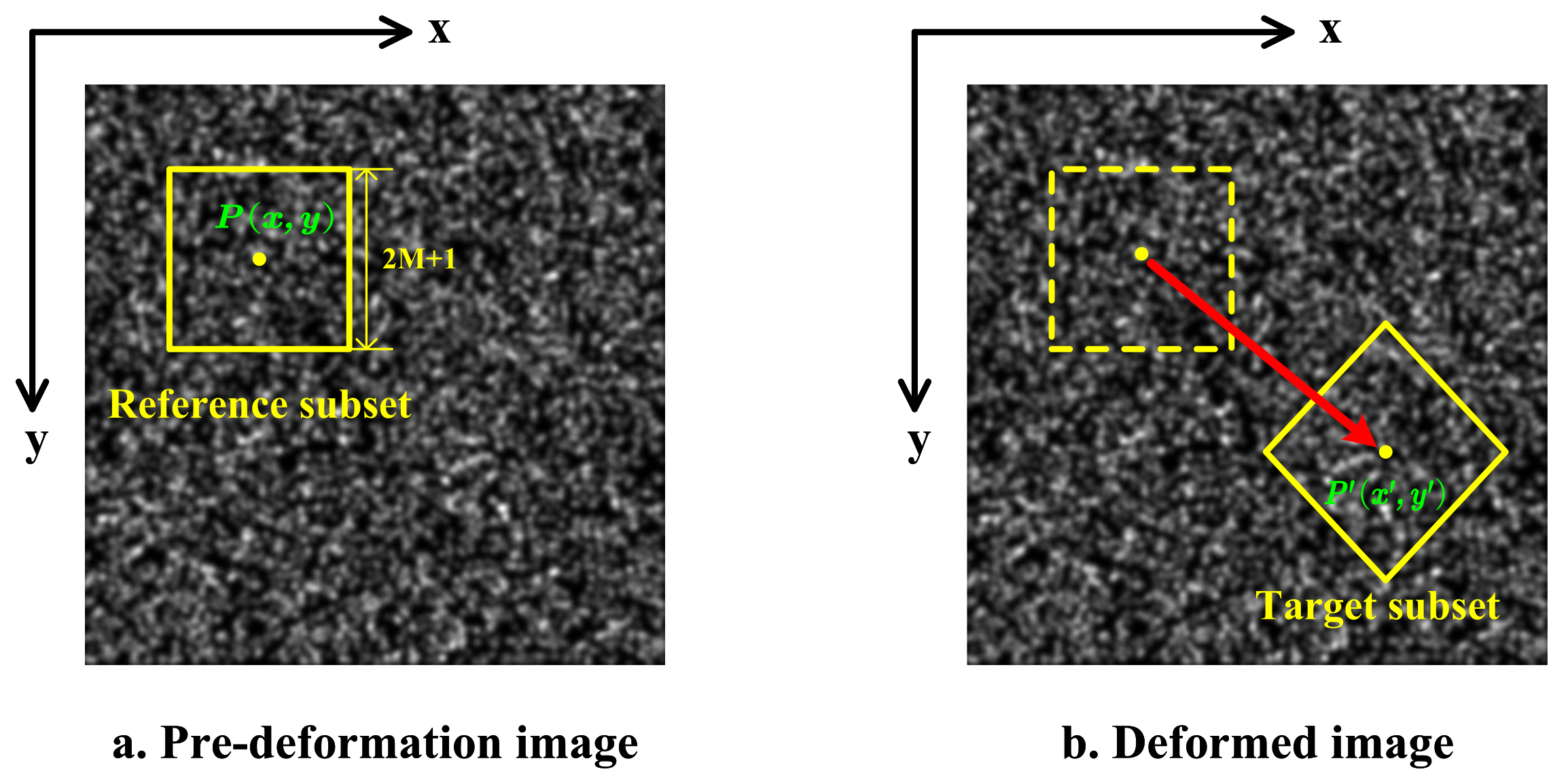
2.1. Related Principles of Integer-Pixel Search

The related principle of DSCM’s integer-pixel search is shown in Figure 1. The speckle image of an object before deformation is recorded as the reference image, and the speckle image of the object after the deformation is recorded as the target image. Any subset of the reference image of size $\left(2M+1\right)\times \left(2M+1\right)$ is selected (e.g., the area surrounded by a yellow rectangular in Figure 1a), and then a matching subset of the target image with the same size is searched (e.g., the area bounded by the yellow solid rectangle in Figure 1b). The integer-pixel displacement is obtained through the calculation of correlation functions in this process.

Figure 1. Related principles of integer-pixel search: (a) pre-deformation image; (b) deformed image.

Common correlation functions are usually based on cross-correlation and distance-based correlation. Based on the cross-correlation function, there are cross-correlation function (CC), normalized cross-correlation function (NCC) and zero-mean normalized cross-correlation function (ZNCC). The distance-based cross-correlation functions are sum of squared distance correlation function (SSD), normalized sum of squared distance correlation function (NSSD) and zero-mean normalized sum of squared distance correlation function (ZNSSD). CC and SSD functions are more sensitive to light intensity changes and light shifts, while NCC and NSSD are more sensitive to light shifts. These four functions have poor anti-interference. On the other hand, ZNCC and ZNSSD have been de-averaged and normalized, which are insensitive to light intensity changes and light shifts and have high anti-interference and stability [52,53]. At the same time, ZNCC is computationally efficient and ZNSSD facilitates derivation and first-order Taylor expansion [42]. To sum up, these two correlation functions are selected in this paper to be applied in the algorithm of integer-pixel and sub-pixel displacement search, respectively. The expressions of these two functions are shown in Equations (1) and (2):

$$C_{ZNCC}=\sum _{i=-M}^M\sum _{j=-M}^M\left[\frac{\left[f\left(x_i,y_j\right)-\overline{f}\right]\times \left[g\left({x_i}^{\prime },{y_j}^{\prime }\right)-\overline{g}\right]}{\mathsf{\Delta }f\times \mathsf{\Delta }g}\right]$$

(1)

$$C_{ZNSSD}=\sum _{i=-M}^M\sum _{j=-M}^M{\left[\frac{f\left(x_i,y_j\right)-\overline{f}}{\mathsf{\Delta }f}-\frac{g\left({x_i}^{\prime },{y_j}^{\prime }\right)-\overline{g}}{\mathsf{\Delta }g}\right]}^2$$

(2)

where M is the pixel spacing from the center of a subset of the selected reference image to any of its edges; $f\left(x_i,y_j\right)$ represents the gray value of the pixel with coordinate $\left(x_i,y_j\right)$ in the reference subset, $g\left({x_i}^{\prime },{y_j}^{\prime }\right)$ is the gray value of the pixel with coordinate $\left({x_i}^{\prime },{y_j}^{\prime }\right)$ in the target subset and $\overline{f}$ and $\overline{g}$ are the average of gray values of all pixels of reference subset and target subset, respectively, the calculation formulas of $\mathsf{\Delta }f$ and $\mathsf{\Delta }g$ are shown in Equations (3) and (4):

$$\mathsf{\Delta }f=\sqrt{\sum _{i=-M}^M\sum _{j=-M}^M{\left[f\left(x_i,y_j\right)-\overline{f}\right]}^2}$$

(3)

$$\mathsf{\Delta }g=\sqrt{\sum _{i=-M}^M\sum _{j=-M}^M{\left[g\left(x_i^{\prime },y_j^{\prime }\right)-\overline{g}\right]}^2}$$

(4)

At the same time, the two are equivalent to each other and satisfy the relation $C_{ZNSSD}=2\times \left(1-C_{ZNCC}\right)$. Among them, the value range of $C_{ZNCC}$ is $\left[-1,1\right]$, when $C_{ZNCC}=0$, it means that the similarity between the reference subset and the target subset is zero, when $C_{ZNCC}=1$, it means that the similarity between the reference subset and the target subset is the greatest, and when $C_{ZNCC}=-1$, it means that the negative similarity between the reference subset and the target subset is maximum. Thus, our goal is to search for a subset of targets in the target image that makes $C_{ZNCC}$ as large as possible or $C_{ZNSSD}$ as small as possible.

2.2. Coarse and Fine Search Algorithm

The coarse and fine search algorithm is an improved algorithm based on the point-by-point search method. It is widely used as the most classic integer-pixel search algorithm. The basic steps are as follows: First, starting from the upper left corner of the region of interest (ROI) of the target image, the maximum search step is selected as 4 pixel, and all the correlation coefficients $C_{ZNCC}$ in the matching area are calculated horizontally and then vertically with the maximum search step as the interval, and the point with the largest $C_{ZNCC}$ is taken as the coarse matching point. Next, the coarse matching point is selected as the center point, and the point with the largest $C_{ZNCC}$ is taken as the fine matching point in the rectangular area of 5 pixel × 5 pixel. Finally, with the fine matching point taken as the center point, the point with the largest $C_{ZNCC}$ is found as the integer-pixel matching point in the rectangular area of 3 pixel × 3 pixel.

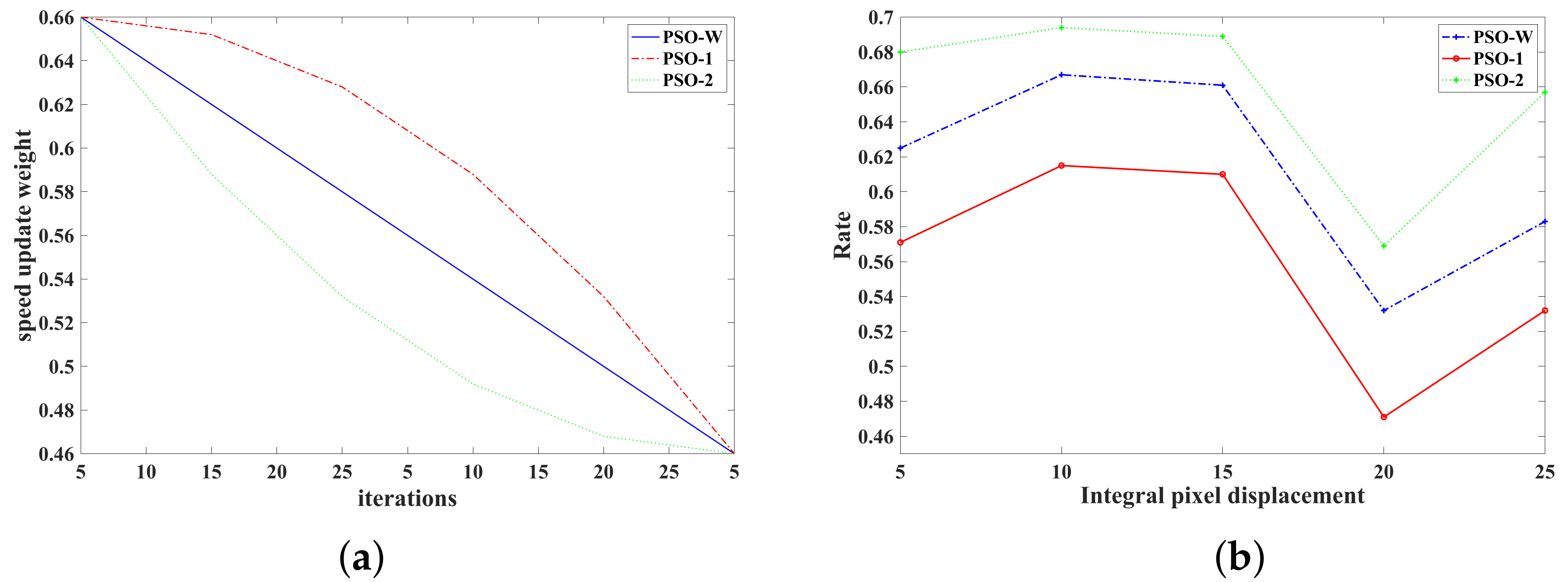
2.3. PSO-W Algorithm

Wu et al. [36] proposed a PSO-based integer pixel search algorithm, denoted as PSO-W, which aims to obtain the integer pixel displacement values, and the main ideas are as follows:

• Customize the integer-pixel position and velocity of the initial particles, where the fitness value of each particle is the correlation coefficient calculated by Equation (1), and set the iteration termination parameters as: trustworthy threshold $C_{trust}=0.75$, maximum iteration number $G_{max}=5$.
• Update the velocities and positions of all particles with the linear inertia weight (see Equation (5)), and keep the velocities and positions of the particles within the search range. If exceeds the specified search range, set the positions and velocities to their proximity boundaries. The particle updated velocity and position formulas are shown in Equations (6) and (7).

  $$w\left(t\right)=0.9-\frac{t}{2G_{max}}$$

  (5)

  $$v_{id}\left(t+1\right)=w\left(t\right)v_{id}\left(t\right)+c_1{r}_1\left[pbes{t}_{id}-p_{id}\left(t\right)\right]+c_2{r}_2\left[gbes{t}_{id}-v_{id}\left(t\right)\right]$$

  (6)

  $$p_{id}\left(t+1\right)=p_{id}\left(t\right)+v_{id}\left(t+1\right)$$

  (7)

  where, t represents the current generation, and $t+1$ represents the next generation, $v_{id}$ is the velocity of the i-th particle in the d direction, and $p_{id}$ is the position of the i-th particle in the d direction. When $d=1$, it flies in the X direction, and when $d=2$, it flies in the Y direction. $c_1$ and $c_2$ are positive acceleration coefficients, respectively. $r_1$ and $r_2$ are two uniform random variables between 0 and 1. $pbest$ is the position where the particle finds the maximum fitness value $C_{pbest}$, and $gbest$ is the position of the maximum fitness value $C_{gbest}$ in the particle swarm, which is a global optimal position.
• For each particle, if the current fitness value is greater than the previous $C_{pbest}$, update it. For the entire population, if the current fitness value is greater than the previous $C_{gbest}$, then update.
• The algorithm terminates until either $C_{pbest}$ is greater than $C_{trust}$ or $G_{maxt}$ is reached. Then output $C_{gbest}$ and its corresponding displacement vector $d_0=\left(u_0,v_0\right)$, otherwise go back to step 2.
• If $C_{d_0}\ge 0.9$, the block-based gradient descent search (BBGDS) algorithm will not be executed. Otherwise, take $d_0$ as the starting point of the BBGDS algorithm, and finally output the integer-pixel with the largest correlation coefficient in the center.

2.4. Sub-Pixel Reconstruction

The integer-pixel displacement cannot meet the requirement of accuracy, which requires the subsequent sub-pixel displacement search. As the key to sub-pixel displacement search, the reconstruction method of sub-pixels usually includes interpolation and fitting methods. In this paper, the gray value of sub-pixel image is reconstructed by gray interpolation method. Common interpolation methods include: the nearest field interpolation method based on one integer-pixel [54], the bilinear interpolation method based on four integer-pixels [37] and the bicubic interpolation method based on sixteen integer-pixels [18,33,42,43]. In this paper, the more commonly used bicubic interpolation method is used to reconstruct sub-pixels.

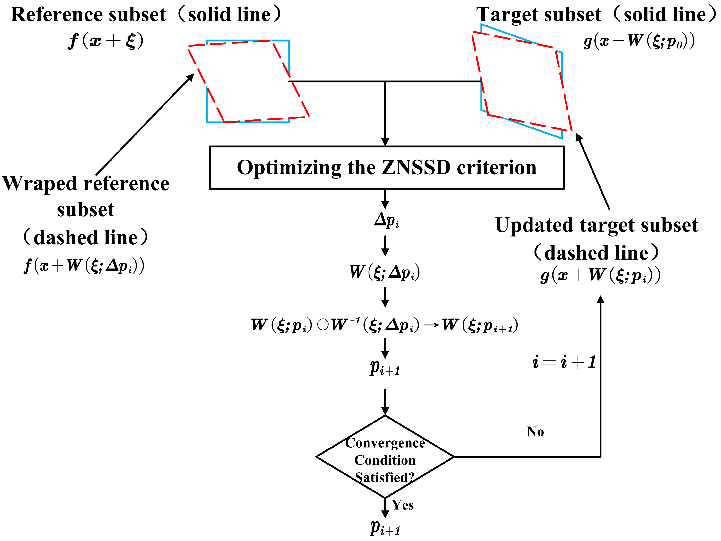
2.5. IC-GN Algorithm

IC-GN sub-pixel search principle is shown in Figure 2, $W\left(\xi ;p_i\right)$ is the Wrap function, which describes the position and shape of the target subset relative to the reference subset. $W\left(\xi ;\mathsf{\Delta }{p}_i\right)$ is the deformation incremental shape function, which acts on the reference sub-region. The shape functions $W\left(\xi ;p_i\right)$ and $W\left(\xi ;\mathsf{\Delta }{p}_i\right)$ are shown in Equations (8) and (9):

$$W\left(\xi ;p_i\right)=\left[\begin{array}{ccc}l1+u{\left(i\right)}_x& u{\left(i\right)}_y& u\left(i\right)\\ v{\left(i\right)}_x& 1+v{\left(i\right)}_y& v\left(i\right)\\ 0& 0& 1\end{array}\right]\left(\begin{array}{c}\mathsf{\Delta }x\\ \mathsf{\Delta }y\\ 1\end{array}\right)$$

(8)

$$W\left(\xi ;\mathsf{\Delta }{p}_i\right)=\left[\begin{array}{ccc}l1+\mathsf{\Delta }u{\left(i\right)}_x& \mathsf{\Delta }u{\left(i\right)}_y& \mathsf{\Delta }u\left(i\right)\\ \mathsf{\Delta }v{\left(i\right)}_x& 1+\mathsf{\Delta }v{\left(i\right)}_y& \mathsf{\Delta }v\left(i\right)\\ 0& 0& 1\end{array}\right]\left(\begin{array}{c}\mathsf{\Delta }x\\ \mathsf{\Delta }y\\ 1\end{array}\right)$$

(9)

where $p_i={\left(u\left(i\right),u{\left(i\right)}_x,u{\left(i\right)}_y,v\left(i\right),v{\left(i\right)}_x,v{\left(i\right)}_y\right)}^T$, $p_i$ represents the deformation vector obtained by the i-th calculation, $u\left(i\right)$ and $v\left(i\right)$ are the i-th calculation results of the reference subset relative to the target subset in the u and v directions, respectively, and $u{\left(i\right)}_x$, $u{\left(i\right)}_y$, $v{\left(i\right)}_x$ and $v{\left(i\right)}_y$ are the i-th calculation results of the first derivative of x and y in the u and v directions, respectively. $\xi ={\left(\mathsf{\Delta }x,\mathsf{\Delta }y,1\right)}^T$, and $\left(\mathsf{\Delta }x,\mathsf{\Delta }y\right)$ are the local coordinates with the center point of the reference subset as the origin. $\mathsf{\Delta }{p}_i={\left(\mathsf{\Delta }u\left(i\right),\mathsf{\Delta }u{\left(i\right)}_x,\mathsf{\Delta }u{\left(i\right)}_y,\mathsf{\Delta }v\left(i\right),\mathsf{\Delta }v{\left(i\right)}_x,\mathsf{\Delta }v{\left(i\right)}_y\right)}^T$, and $\mathsf{\Delta }{p}_i$ denotes the i-th computed deformation increment in the iterative process.

Figure 2. IC-GN sub-pixel search flow chart.

When IC-GN algorithm is initialized, the roles of the target subset and the reference subset are reversed. After applying $W\left(\xi ;\mathsf{\Delta }{p}_0\right)$ to the reference subset (shown in the dashed box on the left in Figure 2), the target subset with the deformation function $W\left(\xi ;p_0\right)$ applied (shown in the solid box on the right in Figure 2) is based on the $C_{ZNSSD}$ correlation criterion function for comparison, that is, $\mathsf{\Delta }{p}_0$ can be obtained by deriving $C_{ZNSSD}$. Then, the generalized inverse matrix $W^{-1}\left(\xi ;\mathsf{\Delta }{p}_0\right)$ of the incremental shape function $W\left(\xi ;\mathsf{\Delta }{p}_0\right)$ is composed of the current estimate $W\left(\xi ;p_0\right)$ to generate the updated shape function $W\left(\xi ;p_1\right)$ of the applied target subset. Next, apply $W\left(\xi ;\mathsf{\Delta }{p}_1\right)$ to the reference subset and apply the deformation function $W\left(\xi ;p_1\right)$ to the target subset based on the $C_{ZNSSD}$ correlation criterion function to obtain $\mathsf{\Delta }{p}_1$... Iteratively solve $\mathsf{\Delta }{p}_i$ and $p_{i+1}$ until the convergence condition is met, that is, $\parallel \mathsf{\Delta }{p}_i\parallel \le 0.001$ or the number of iterations reaches a specified value, and finally the deformation vector $p_{i+1}$ is output.

Among them, $C_{ZNSSD}\left(\mathsf{\Delta }{p}_i\right)$, $\mathsf{\Delta }{p}_i$, $W\left(\xi ;p_{i+1}\right)$ and $\parallel \mathsf{\Delta }{p}_i\parallel$ are shown as Equations (10), (11), (13) and (14). $W^{-1}\left(\xi ;\mathsf{\Delta }{p}_i\right)$ is the generalized inverse matrix of $W\left(\xi ;\mathsf{\Delta }{p}_i\right)$, and the combined transformation of the two shape functions is denoted as “∘”.

$$C_{ZNSSD}\left(\mathsf{\Delta }{p}_i\right)=\sum _{\xi }{\left\{\frac{\left[f\left(x+W\left(\xi ;\mathsf{\Delta }{p}_i\right)\right)-\overline{f}\right]}{\mathsf{\Delta }f}-\frac{\left[g\left(x+W\left(\xi ;p_i\right)\right)-\overline{g}\right]}{\mathsf{\Delta }g}\right\}}^2$$

(10)

$$\mathsf{\Delta }{p}_i=-H^{-1}\times \sum _{\xi }\left\{{\left(\nabla f\frac{\partial W}{\partial p_i}\right)}^T\times \left[\left(f\left(x+\xi \right)-\overline{f}\right)-\frac{\mathsf{\Delta }f}{\mathsf{\Delta }g}\left(g\left(x+W\left(\xi ;p_i\right)\right)-\overline{g}\right)\right]\right\}$$

(11)

H is a 6th-order square matrix, and the expression is Equation (12):

$$H=\sum _{\xi }\left[{\left(\nabla f\frac{\partial W}{\partial p_i}\right)}^T\times \left(\nabla f\frac{\partial W}{\partial p_i}\right)\right]$$

(12)

$\frac{\partial W}{\partial p_i}=\left(\begin{array}{cccccc}1& \mathsf{\Delta }x& \mathsf{\Delta }y& 0& 0& 0\\ 0& 0& 0& 1& \mathsf{\Delta }x& \mathsf{\Delta }y\end{array}\right)$ is the Jacobian matrix of the shape function, $\nabla f$ is the gray gradient value of each pixel in the reference subset, $\frac{\partial W}{\partial p_i}$ and $\nabla f$ are only related to the reference image and will not change with iteration.

$$W\left(\xi ;p_i\right)\circ W^{-1}\left(\xi ;\mathsf{\Delta }{p}_i\right)\to W\left(\xi ;p_{i+1}\right)$$

$$=\left[\begin{array}{ccc}1+u{\left(i\right)}_x& u{\left(i\right)}_y& u\left(i\right)\\ v{\left(i\right)}_x& 1+v{\left(i\right)}_y& v\left(i\right)\\ 0& 0& 1\end{array}\right]{\left[\begin{array}{ccc}1+\mathsf{\Delta }u{\left(i\right)}_x& \mathsf{\Delta }u{\left(i\right)}_y& \mathsf{\Delta }u\left(i\right)\\ \mathsf{\Delta }v{\left(i\right)}_x& 1+\mathsf{\Delta }v{\left(i\right)}_y& \mathsf{\Delta }v\left(i\right)\\ 0& 0& 1\end{array}\right]}^{-1}\left(\begin{array}{c}\mathsf{\Delta }x\\ \mathsf{\Delta }y\\ 1\end{array}\right)$$

(13)

$$\parallel \mathsf{\Delta }p\parallel =\sqrt{{\left(\mathsf{\Delta }u\right)}^2+{\left(\mathsf{\Delta }x\times \mathsf{\Delta }{u}_x\right)}^2+{\left(\mathsf{\Delta }y\times \mathsf{\Delta }{u}_y\right)}^2+{\left(\mathsf{\Delta }v\right)}^2+{\left(\mathsf{\Delta }x\times \mathsf{\Delta }{v}_x\right)}^2+{\left(\mathsf{\Delta }y\times \mathsf{\Delta }{v}_y\right)}^2}$$

(14)

Let

$$W\left(p_{i+1}\right)=\left[\begin{array}{ccc}1+u{\left(i\right)}_x& u{\left(i\right)}_y& u\left(i\right)\\ v{\left(i\right)}_x& 1+v{\left(i\right)}_y& v\left(i\right)\\ 0& 0& 1\end{array}\right]{\left[\begin{array}{ccc}1+\mathsf{\Delta }u{\left(i\right)}_x& \mathsf{\Delta }u{\left(i\right)}_y& \mathsf{\Delta }u\left(i\right)\\ \mathsf{\Delta }v{\left(i\right)}_x& 1+\mathsf{\Delta }v{\left(i\right)}_y& \mathsf{\Delta }v\left(i\right)\\ 0& 0& 1\end{array}\right]}^{-1}$$

(15)

then

$$p_{i+1}={\left[\left(1,0,0\right)W\left(p_{i+1}\right)\left(\begin{array}{cccccc}0& 0& 1& 0& 0& 0\\ 0& 0& 0& 1& 0& 0\\ 1& 0& 0& 0& 0& 0\end{array}\right)+\left(0,1,0\right)W\left(p_{i+1}\right)\left(\begin{array}{cccccc}0& 0& 0& 0& 1& 0\\ 0& 0& 0& 0& 0& 1\\ 0& 1& 0& 0& 0& 0\end{array}\right)-\left(0,0,1,0,0,1\right)\right]}^T$$

(16)

2.6. Generate Simulated Speckle Images

In order to verify the results of the algorithms, computer-generated speckle images proposed by Zhou [38] are used for the simulation verification in this paper. The gray scale $I_1\left(x,y\right)$ and $I_2\left(x,y\right)$ of the speckle images generated before and after the deformation are shown in the Equation (17).

$$\left\{\begin{array}{c}{I}_1\left(x,y\right)=\sum _{k=1}^n{I}_0{e}^{-\frac{{\left(x-x_k\right)}^2+{\left(y-y_k\right)}^2}{R^2}}\hfill \\ I_2\left(x,y\right)=\sum _{k=1}^n{I}_0{e}^{-\frac{{\left(x-x_k^{\prime }\right)}^2+{\left(y-y_k^{\prime }\right)}^2}{R^2}}\hfill \end{array}\right.$$

(17)

Among them, $I_0$ is the light intensity at the center of the speckle, n is the number of speckles, R is the radius of the speckle,$\left(x_k,y_k\right)$ is the spot center position of the speckle pattern before randomly generated deformation and $\left(x_k^{\prime },y_k^{\prime }\right)$ is the center position of the speckle pattern after the deformation.

$$\left\{\begin{array}{c}{x}_k^{\prime }=x_k+u+x_k{u}_x+y_k{u}_y\hfill \\ y_k^{\prime }=y_k+v+x_k{v}_x+y_k{v}_y\hfill \end{array}\right.$$

(18)

In Equation (18), u and v are the rigid body displacements of the speckle, and $u_x$, $u_y$, $v_x$ and $v_y$ are the first derivatives of the displacements in the u and v directions with respect to x and y, respectively.

2.7. Algorithm Performance Evaluation Index

In this paper, the algorithms are evaluated in terms of computational accuracy and efficiency. The computational accuracy is evaluated quantitatively using two metrics: the mean error and the root mean square error (RMSE). The mean error in the u direction ($u_e$) is defined as Equation (19):

$$u_e=\frac{1}{n}\sum _{i=1}^n\left(u_i-u_d\right)$$

(19)

where n represents the number of center points of the sub-area, and $u_i$ represents the calculated displacement value at the i-th POI, $u_d$ denotes the actual imposed sub-pixel displacement. RMSE is defined as Equation (20):

$$RMSE=\sqrt{\frac{1}{n}\sum _{i=1}^n\left(u_i-\overline{u}\right)}$$

(20)

where $\overline{u}=\frac{1}{n}{\sum }_{i=1}^n{u}_i$.

The efficiency of an algorithm is quantitatively expressed by the average number of iterations of the algorithm.

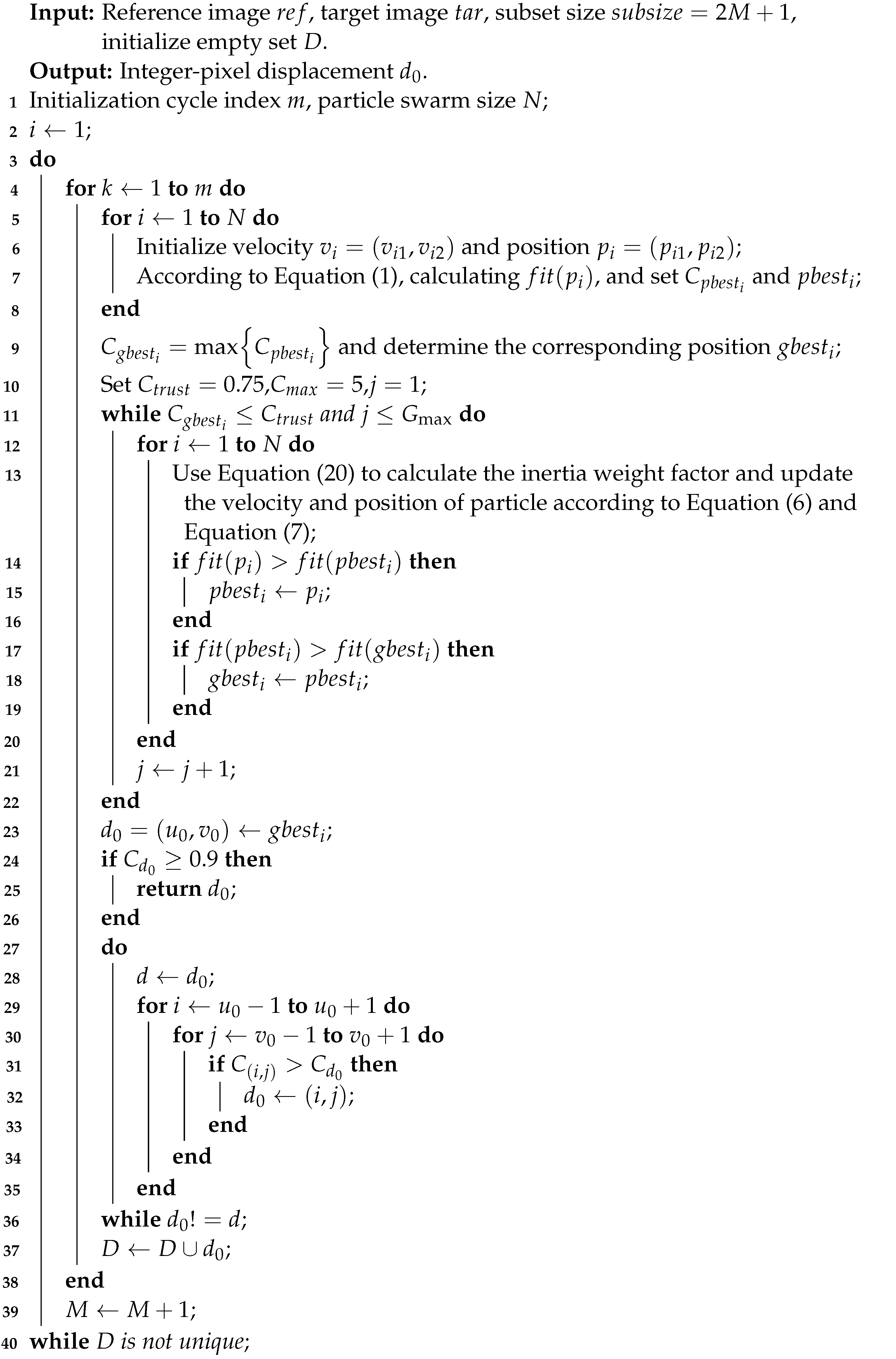
3. Improved PSO-Based Efficient Integer-Pixel Displacement Search Algorithm

The PSO-W algorithm provides technical support for real-time measurement of displacement at a rate of up to 60 fps (frames per second) with guaranteed accuracy of the algorithm [36]; however, it also has the following two problems that can be improved.

1.

The maximum value is not unique

It is easy to obtain, from Equation (1), if and only if $\forall i,j\in \left[-M,M\right],f\left(x_i,y_j\right)-\overline{f}=\lambda \left(g\left({x_i}^{\prime },{y_j}^{\prime }\right)-\overline{g}\right)$, $\lambda \ne 0$, Equation (21) holds.

$$\sum _{i=-M}^M\sum _{j=-M}^M\left[\left[f\left(x_i,y_j\right)-\overline{f}\right]\times \left[g\left({x_i}^{\prime },{y_j}^{\prime }\right)-\overline{g}\right]\right]=\mathsf{\Delta }f\times \mathsf{\Delta }g$$

(21)

where M is usually between 10 and 30 [47]. So there is a problem that $d_0$ is not unique when $C_{gbest}$ is searched. As shown in Figure 3, using the method in Section 2.6 of this paper (take $I_0=80$, $n=2000$, $ROI=512$ pixel × 512 pixel, $R=2$ pixel) randomly generated speckle images, the left side is the reference image and the right side is the target image. Let $M=10$, at this time the $C_{ZNCC}$ of subset center points $A\left(307,61\right)$ and $B\left(123,365\right)$ is 1.

Figure 3. Speckle pattern.

The best way to solve this problem is to increase the number of speckles when making the speckle image or increase the size of the searching subset after the speckle image is determined. As in the previous example, if M is increased from 10 to 16, only unique values exist.

2.

Using linear inertia weighting factors

The weight factor is used to update the position vector and velocity vector of the particles. The inertia weight factor in the PSO-W algorithm is linear, so the influence of the non-linear inertia weight factor on the particles can be considered. The algorithm for modifying the inertia weight factor of Equation (5) into inertia weights shown in Equations (22) and (23) is denoted as PSO-1 and PSO-2, respectively.

$$w\left(t\right)=w_s-\left(w_s-w_e\right)\times {\left(\frac{t}{maxgen}\right)}^2$$

(22)

$$w\left(t\right)=w_s-\left(w_s-w_e\right)\times \left[\frac{2t}{maxgen}-{\left(\frac{t}{maxgen}\right)}^2\right]$$

(23)

Among them, $w\left(t\right)$ is the inertia weight when the number of iterations is t, $w_s$ is the initial inertia weight, $w_e$ is the inertia weight when the number of iterations reaches the maximum number of iterations and max $gen$ is the maximum number of iterations. The curves of PSO-1, PSO-2 and PSO-W inertia weighting factors with the number of iterations are shown in Figure 4a.

Figure 4. Three algorithms comparison of inertia weight factors with the number of iterations (a) and search efficiency (b).

Due to the fact that the above maximum value is not unique, the number of speckles in the speckle image is increased in the simulation experiment, and the speckle image before deformation is generated as shown in Figure 5. In order to compare the efficiency of the PSO-W, PSO-1 and PSO-2 algorithms, the above-mentioned speckle image was taken as the reference image, and then five pixels are translated along the horizontal direction for each step, and the continuous movement is five steps. Each step generates a speckle image. There are a total of five images, which are used as the target image, and an integer pixel search is performed for the reference image and each target image. Finally, we use the coarse and fine search method as the reference to compare the search efficiency of the integer-pixel of the aforementioned three algorithms.

Figure 5. Speckle image before deformation.

As shown in Figure 4b, the ratio of the search times of the three algorithms to the search times of the coarse and fine search algorithms varies with the value of the whole pixels displacement. As can be seen from the figure, in the best case, the efficiency of the PSO-1 algorithm is 52.9% higher than that of the coarse and fine search algorithm and 11.5% higher than that of the PSO-W algorithm. In the worst case, the efficiency of the PSO-1 algorithm is 38.5% higher than that of the coarse and fine search algorithm and 7.7% higher than that of the PSO-W algorithm. In general, the search efficiency of PSO-1 algorithm is 8.8% higher than that of PSO-W on average. Finally, according to the experiment, it is concluded that the search efficiency of the PSO-1 algorithm is the highest.

Therefore, the PSO-1 algorithm, which is shown in Algorithm 1, is chosen as the optimal integer-pixel search algorithm in this paper.

Algorithm 1: PSO-1.

4. Sub-Pixel Displacement Search Algorithm

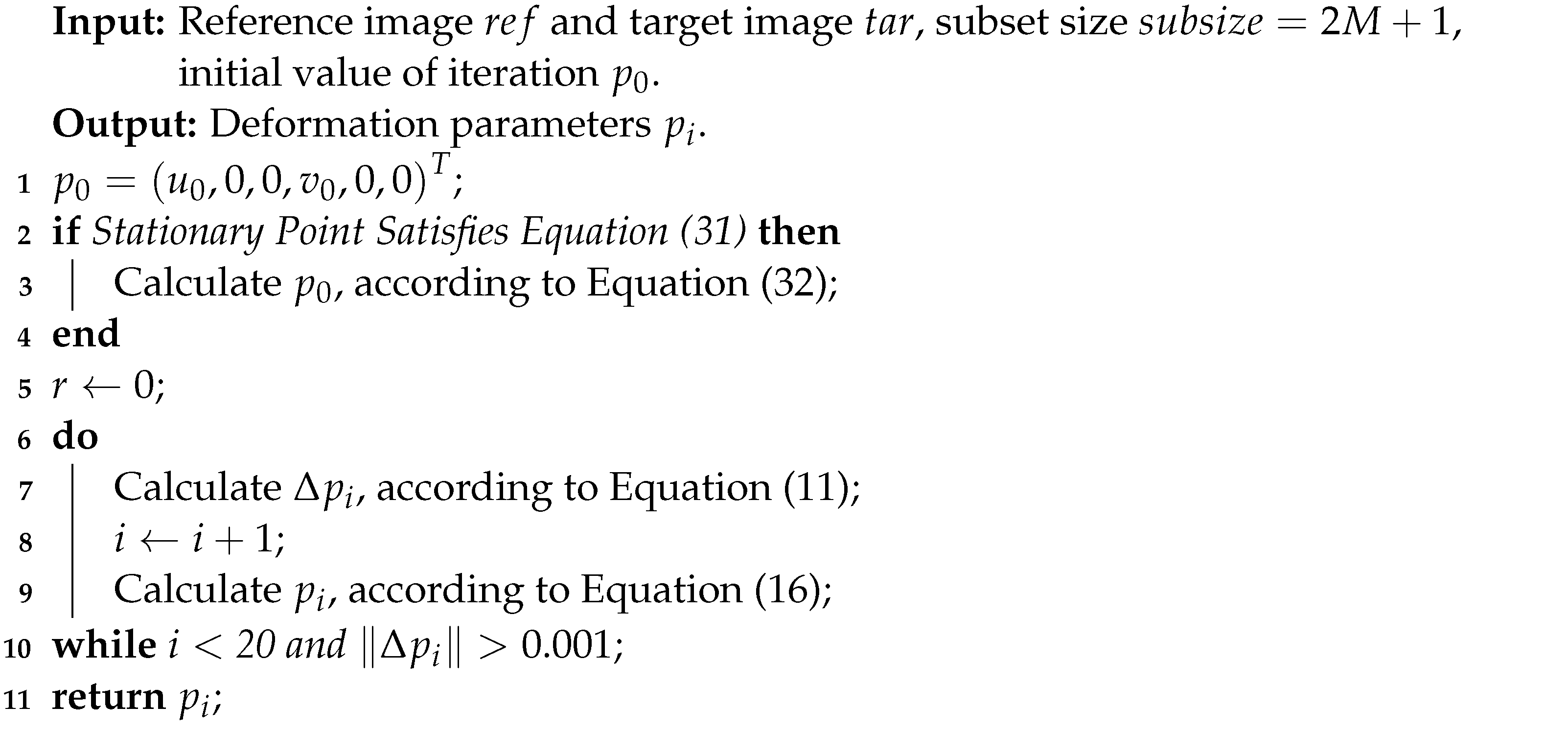
4.1. Improved Sub-Pixel Displacement Search Algorithm IV-ICGN

The initial value of the iteration of IC-GN algorithm is the point $p_0={\left(u_0,0,0,v_0,0,0\right)}^T$, which is the position of an integer-pixel from integer-pixel search algorithm [33,36,42]. We found that this initial value can be further refined by replacing it with sub-pixel values, and the accuracy and efficiency of sub-pixel displacement search can be improved accordingly.

Using the PSO-1 algorithm we can match the displacement of the integer-pixel point $I_0$ with the correlation coefficient $C_0$. As shown in Figure 6, take 8 adjacent integer-pixel points $I_i\left(i=1,2,...,8\right)$ around $I_0$, and their correlation coefficients are $C_i\left(i=1,2,...,8\right)$, respectively. With $I_0$ as the origin, a relative coordinate system $U-V$ is established. The coordinates of each point are shown in the figure.

Figure 6. Quadratic surface fitting coordinate diagram.

The quadratic surface fitting has the following advantages, one is to facilitate the determination of maximum points, and the other is to have a unified analytical solution to facilitate calculation. The quadric surface fitting is performed on the above nine points, and the fitting function is as follows:

$$C\left(u,v\right)=a_0+a_{1}u+a_{2}v+a_3{u}^2+a_{4}uv+a_5{v}^2$$

(24)

Next, the least square method is used to solve the coefficients $a_0$, $a_1$, $a_2$, $a_3$, $a_4$, $a_5$. The coordinates of point $I_i\left(i=0,1,2,...,8\right)$ in the aforementioned $U-V$ coordinate system are $\left(u_i,v_i\right)$, and the fitting error is recorded as $e_i\left(a_0,a_1,a_2,a_3,a_4,a_5\right)$ in Equation (25)

$$e_i\left(a_0,a_1,a_2,a_3,a_4,a_5\right)=C\left(u_i,v_i\right)-C_i=a_0+a_1{u}_i+a_2{v}_i+a_3{u}_i^2+a_4{u}_i{v}_i+a_5{v}_i^2-C_i$$

(25)

Then the sum of squared errors $E\left(a_0,a_1,a_2,a_3,a_4,a_5\right)$ is

$$E\left(a_0,a_1,a_2,a_3,a_4,a_5\right)=\sum _{i=0}^8{\left(C\left(u_i,v_i\right)-C_i\right)}^2$$

(26)

Calculate the first-order partial derivatives of $a_0$, $a_1$, $a_2$, $a_3$, $a_4$ and $a_5$ form Equation (26) and set them equal to 0 to obtain Equation (27).

$$\left\{\begin{array}{c}\sum _{i=0}^8{e}_i=0\hfill \\ \sum _{i=0}^8{e}_i{u}_i=0\hfill \\ \sum _{i=0}^8{e}_i{v}_i=0\hfill \\ \sum _{i=0}^8{e}_i{u}_i^2=0\hfill \\ \sum _{i=0}^8{e}_i{u}_i{v}_i=0\hfill \\ \sum _{i=0}^8{e}_i{u}_i^2=0\hfill \end{array}\right.$$

(27)

Let $\overline{C}=\frac{1}{9}{\sum }_{i=0}^8{C}_i$, $\overline{Cv}=\frac{1}{9}{\sum }_{i=0}^8{C}_i{v}_i$, $\overline{Cv}=\frac{1}{9}{\sum }_{i=0}^8{C}_i{v}_i$, $\overline{C{u}^2}=\frac{1}{9}{\sum }_{i=0}^8{C}_i{u}_i^2$, $\overline{C{v}^2}=\frac{1}{9}{\sum }_{i=0}^8{C}_i{v}_i^2$, $\overline{Cuv}=\frac{1}{9}{\sum }_{i=0}^8{C}_i{u}_i{v}_i$. From the coordinates of each point in Figure 5, with further optimization, we obtain Equation (28):

$$\left[\begin{array}{cccccc}1& 0& 0& \frac{2}{3}& 0& \frac{2}{3}\\ 0& \frac{2}{3}& 0& 0& 0& 0\\ 0& 0& \frac{2}{3}& 0& 0& 0\\ \frac{2}{3}& 0& 0& \frac{2}{3}& 0& \frac{4}{9}\\ 0& 0& 0& 0& \frac{4}{9}& 0\\ \frac{2}{3}& 0& 0& \frac{4}{9}& 0& \frac{2}{3}\end{array}\right]\left[\begin{array}{c}{a}_0\hfill \\ a_1\hfill \\ a_2\hfill \\ a_3\hfill \\ a_4\hfill \\ a_5\hfill \end{array}\right]=\left[\begin{array}{c}\overline{C}\hfill \\ \overline{Cu}\hfill \\ \overline{Cv}\hfill \\ \overline{C{u}^2}\hfill \\ \overline{Cuv}\hfill \\ \overline{C{v}^2}\hfill \end{array}\right]$$

(28)

Solving Equation (27), we can obtain $a_0=5\overline{C}-3\overline{C{u}^2}-3\overline{C{v}^2}$, $a_1=\frac{3}{2}\overline{Cu}$, $a_2=\frac{3}{2}\overline{Cv}$, $a_3=\frac{9}{2}\overline{C{u}^2}-3\overline{C}$, $a_4=\frac{9}{4}\overline{Cuv}$, $a_5=\frac{9}{2}\overline{C{u}^2}-3\overline{C}$. Next, the maximum point of the fitting surface is obtained, and the initial value of sub-pixel deformation parameters is further determined. The maximum point of the fitting function $C\left(u,v\right)$ should satisfy Equations (29) and (30):

$$\frac{\partial C\left(u,v\right)}{\partial u}=a_1+2a_{3}u+a_{4}v=0$$

(29)

$$\frac{\partial C\left(u,v\right)}{\partial v}=a_2+a_{4}u+2a_{5}v=0$$

(30)

Find the stagnation point $\left(u^{\prime },v^{\prime }\right)$ as $\left(\frac{2a_1{a}_5-a_2{a}_4}{a_4^2-4a_3{a}_5},\frac{2a_2{a}_3-a_1{a}_4}{a_4^2-4a_3{a}_5}\right)$. Find the second-order partial derivatives of $C\left(u,v\right)$, ${\left.\frac{{\partial }^{2}C\left(u,v\right)}{\partial u^2}\right|}_{\left(u^{\prime },v^{\prime }\right)}=2a_3$, ${\left.\frac{{\partial }^{2}C\left(u,v\right)}{\partial u\partial v}\right|}_{\left(u^{\prime },v^{\prime }\right)}=a_4$, ${\left.\frac{{\partial }^{2}C\left(u,v\right)}{\partial v^2}\right|}_{\left(u^{\prime },v^{\prime }\right)}=2a_5$.

When

$$\left\{\begin{array}{c}{a}_3<0\hfill \\ 4a_3{a}_5-a_4^2>0\hfill \end{array}\right.$$

(31)

holds, the maximum point of the fitted surface is $P\left(\frac{2a_1{a}_5-a_2{a}_4}{a_4^2-4a_3{a}_5},\frac{2a_2{a}_3-a_1{a}_4}{a_4^2-4a_3{a}_5}\right)$, and the initial value of the sub-pixel deformation parameter is

$$p_0={\left(\frac{2a_1{a}_5-a_2{a}_4}{a_4^2-4a_3{a}_5}+u_0,0,0,\frac{2a_2{a}_3-a_1{a}_4}{a_4^2-4a_3{a}_5}+v_0,0,0\right)}^T$$

(32)

Otherwise, when condition (31) does not hold, algorithm IV-ICGN degenerates to IC-GN, $p_0={\left(u_0,0,0,v_0,0,0\right)}^T$. According to the simulation results, IV-ICGN algorithm hardly degenerates into IC-GN. The steps of IV-ICGN algorithm are shown in Algorithm 2.

Algorithm 2: Algorithm IV-ICGN.

4.2. Sub-Pixel Displacement Simulation Experiment

Using the method in Section 2.6 of this paper, take $I_0=80$, $n=8000$, $ROI=512$ pixel × 512 pixel, $R=2$ pixel, to generate a speckle image before deformation as shown in Figure 5 in Section 3, which was used as the reference image. Then move 0.05 pixel in each step along the horizontal u direction, and move continuously for 20 steps. Each step generates a speckle image, and a total of 20 images have been generated and are used as the target image.

Considering the surface fitting (SF) algorithm, grayscale gradient (GG) algorithm and FANR algorithm from the literature [43], IC-GN algorithm and the proposed IV-ICGN algorithm were used to solve the sub-pixel displacement for the reference image and each target image, respectively. The ROI area of each image is divided into sub-regions. According to the experimental results of Section 3, this paper takes the subset size as 33 pixel $\times 33$ pixel, and the adjacent grid spacing in the horizontal u and vertical v directions is five pixels, a total of $96\times 96=9216$ center points, that is, 9216 sub-regions. The iteration termination conditions set by the algorithm are: $\parallel \mathsf{\Delta }p\parallel \le 0.001$ or the maximum number of iterations is 20.

Figure 7 and Figure 8 show the comparison curves of the mean error and the root mean square error of the five algorithms in the u direction with the preset displacement value, respectively. It can be seen from Figure 7 that the overall trend of average errors of all algorithms has a sinusoidal curve distribution, and this pattern is due to the error caused by interpolation when reconstructing sub-pixels [55]. Among them, the mean error and the root mean square error of FANR algorithm, IC-GN algorithm and IV-ICGN algorithm are better than the surface fitting algorithm and grayscale gradient algorithm, and the grayscale gradient algorithm is better than the surface fitting algorithm.

Figure 7. Comparison curve of the mean error in the u direction of five algorithms.

Figure 8. Comparison curve of the RMSE in the u direction of five algorithms.

The maximum and minimum values of the absolute value of the mean error and the maximum value and minimum value of the root mean square error value of the five algorithms are shown in Table 1. From Table 1, we can see that the maximum and minimum values of AVME and RMSE of IV-ICGN algorithm are the smallest, followed by IC-GN, FANR and GG and SF are the largest.

Table 1. Comparison of the absolute value of the mean error and the root mean square error value of the five algorithms.

Algorithm	AVME ($\times {10}^{-3}$ Pixel)		RMSE ($\times {10}^{-3}$ Pixel)
	Minimum	Maximum	Minimum	Maximum
SF	13.8	24.9	16.0	26.9
GG	6.0 0	13.5	8.0 0	15.3
FANR	1.00	4.31	1.0 0	1.38
IC-GN	0.90	4.24	0.97	1.37
IV-ICGN	0.31	3.56	0.90	1.33

The abbreviation AVME is the absolute value of the mean error. The abbreviation RMSE is the root mean square error.

At the same time, in order to compare the mean error and the root mean square error of FANR algorithm, IC-GN algorithm and IV-ICGN algorithm, the comparison curves of these three algorithms are shown in Figure 9 and Figure 10. The mean error and root mean square error distribution of IV-ICGN algorithm are both lower than IC-GN and FANR, and the mean error and root mean square error of IC-GN are similar to FANR. As can be seen from the figure, in the best case, the mean error of the IV-ICGN algorithm is 66.2% lower than that of the IC-GN algorithm, and 69.5% lower than that of the FANR algorithm, the root mean square error of the IV-ICGN algorithm is 15.6% lower than that of the IC-GN algorithm, and 17.1% lower than that of the FANR algorithm. In the worst case, the mean error of IV-ICGN algorithm is 6.0% lower than that of the IC-GN algorithm, and 4.6% lower than that of FANR algorithm, the root mean square error of the IV-ICGN algorithm is 1.4% lower than that of the IC-GN algorithm and 0.3% lower than that of the FANR algorithm. Finally, according to the experimental curve, it is concluded that our algorithm is better than the comparison algorithm IC-GN and FANR with smaller mean error and root mean square error and better calculation accuracy.

Figure 9. Comparison curve of the mean error in the u direction of three algorithm.

Figure 10. Comparison curve of the RMSE in the u direction of three algorithms.

As shown in Figure 11, the number of iterations of the three algorithms, FANR, IC-GN and IV-ICGN, varies with the preset displacement value. It can be seen from the figure that IV-ICGN generally has a smaller iteration time than IC-GN, and the iteration times of the two algorithms increase slowly with the increase in the displacement preset value, while the growth rate decreases slowly. Finally, according to the experimental curve, it is concluded that IV-ICGN is better than FANR and IC-GN in algorithm efficiency.

Figure 11. Comparison curve of number of iterations of algorithm IV-ICGN and algorithm IC-GN.

Therefore, IV-ICGN algorithm is the best of the five algorithms in terms of computational accuracy and algorithm efficiency.

4.3. Real Rigid Body Translation Experiment

The composition of the experimental system is shown in Figure 12. Among them, ① is the glass with speckles, ② is the light source equipment whose maximum light intensity is 5600 lm, ③ is the electronically controlled translation stage, which can apply displacement in the X and Y directions, ④ is the CCD camera. The experiment process is as follows:

Figure 12. Experimental system.

• Making speckles. Clean the glass surface with alcohol first and then spray the matte black paint evenly on the glass surface to form randomly distributed and uniformly sized speckles. During the painting process, keep the distance between the spray gun and the glass constant and vertical.
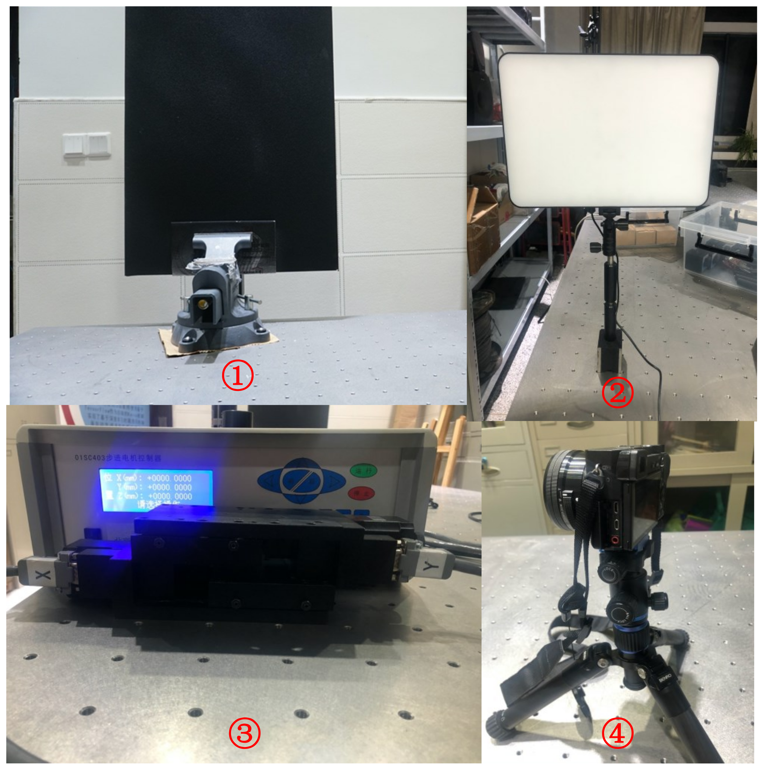
• Fixing the experimental device. The first step is to fix the glass with speckles on the holder. The second step is to fix the electronically controlled translation stage and the light source equipment on the optical platform. The third step is to fix the CCD camera on the electronically controlled translation stage.
• Determine the pixel equivalent of the camera system, which is 0.400 mm/pixel in this experiment.
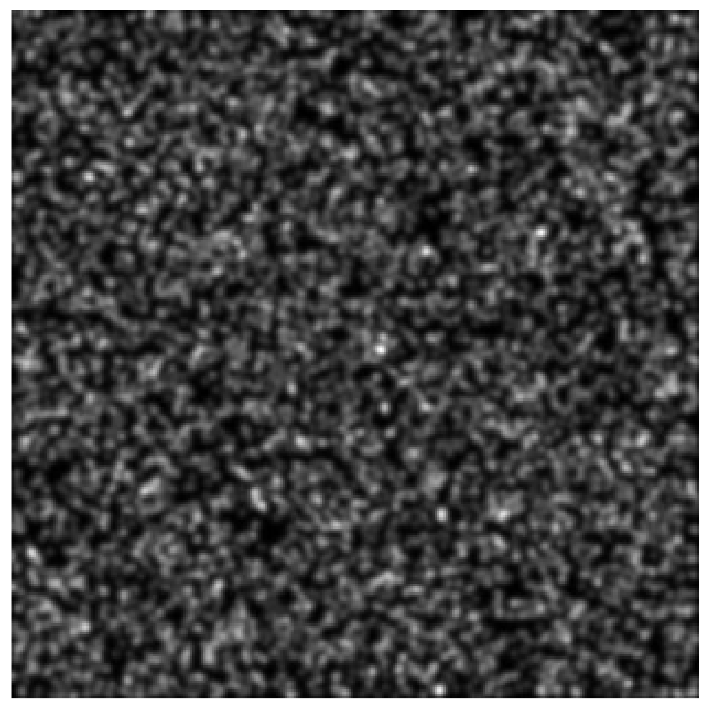
• Collecting speckle images. Firstly, the real speckle image before displacement is acquired as the reference image, as shown in Figure 13, the size of the image is 512 pixel × 512 pixel. Then, several speckle images after the displacements in the X and Y directions, respectively, applied on the electronically controlled translation stage are collected as target images. All images are the region of interest after the surrounding environment and glass edges have been removed, which contains the full-field displacement.
  

  Figure 13. Real speckle image.
• Calculating the pixel displacement value. The proposed algorithm is used to calculate the pixel displacement values, and then compare and analyze the calculated displacement value with the real value.

In this paper, the X direction displacement applied by the electronically controlled translation stage is taken as an example to illustrate the experimental results. The translation is gradually applied to the X-direction with 0.1 mm per step, and a total of 10 steps are moved to obtain 10 target images. The mean value of the sub-pixel displacement is obtained by calculating the center point of each reference subset with the proposed IV-ICGN algorithm, FA-NR algorithm and IC-GN algorithm, and then the absolute values of the mean error obtained by comparing the actual sub-pixel displacement value are shown in Figure 14.

Figure 14. Mean of sub-pixel displacement corresponding to each movement of 0.1 mm.

As shown in Figure 14, there are the absolute values of the mean errors obtained by the IV-ICGN, IC-GN and FA-NR. It can be seen that the absolute value of the mean error of IV-ICGN algorithm is the smallest among the three algorithms, basically between $1\times {10}^{-2}$ pixel and $2\times {10}^{-2}$ pixel, even up to $7\times {10}^{-3}$ pixel. While the other two algorithms are basically between $2\times {10}^{-2}$ pixel and $4\times {10}^{-2}$ pixel; therefore, it can be seen that the IV-ICGN algorithm also has the best performance in the real environment measurement.

5. Discussion

• In the integer pixel search, in view of the two problems of non-unique maximum value and parameter setting in PSO-W [36] algorithm, PSO-1 algorithm with higher search efficiency is proposed. The simulation results show that PSO-1 has higher search efficiency. In terms of sub-pixels, based on IC-GN [42] algorithm with the highest accuracy at present, IV-ICGN algorithm is proposed. Sub-pixel level iterative initial values will make the algorithm converge more easily and with fewer iterations, while improving accuracy and efficiency. The simulation results show that the proposed algorithm has higher precision and higher efficiency than the comparison algorithms.
• However, this study can consider parallel computing to improve computational efficiency. CUDA-based programming can take advantage of the GPU’s parallel computing engine to improve floating-point computing capabilities, thereby improving computing efficiency. At the same time, many floating-point operations are involved in the iterative calculation, and the iterative initial value of multiple points is calculated in parallel to quickly achieve the full-field matching effect.
• At the same time, the research should consider the effect of noise on the algorithm. Although, real experiments show that IV-ICGN algorithm has the best performance; however, we can further improve the accuracy of the algorithm through noise compensation methods. At the same time, we suggest that the results can be compared with some other free 2D DIC software in future work [56].

6. Conclusions

Under the given hardware, high precision and high efficiency have always been what DSCM strives for and pursues; therefore, this paper proposes an improved DSCM algorithm, which is composed of an efficient PSO-1 integer-pixel search algorithm and a higher-precision IV-ICGN sub-pixel search algorithm. The achieved advantages in this paper are as follows:

• The search efficiency of PSO-1 algorithm is higher than that of PSO-W algorithm. In the best case, the efficiency of the PSO-1 algorithm is 52.9% higher than that of the coarse and fine search algorithm, and 11.5% higher than that of the PSO-W algorithm. In the worst case, the efficiency of the PSO-1 algorithm is 38.5% higher than that of the coarse and fine search algorithm and 7.7% higher than that of the PSO-W algorithm. In general, the search efficiency of PSO-1 algorithm is 8.8% higher than that of PSO-W on average.
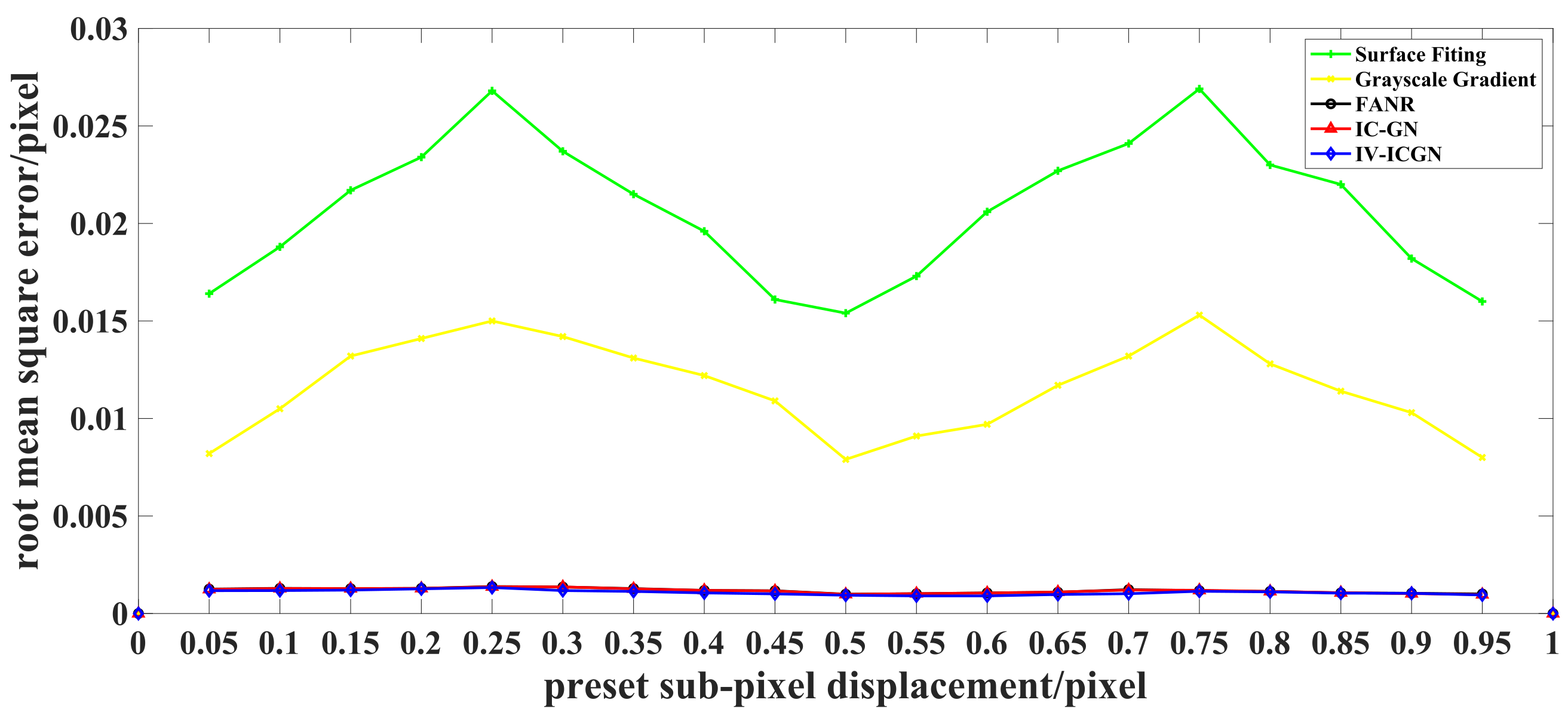
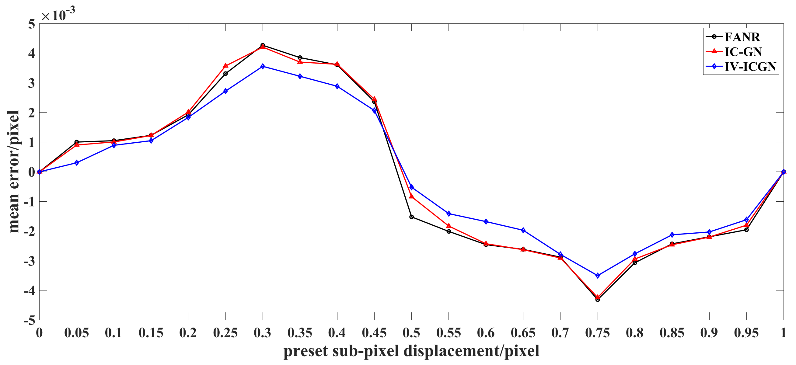
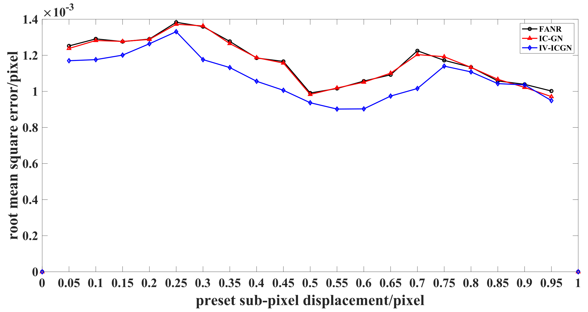
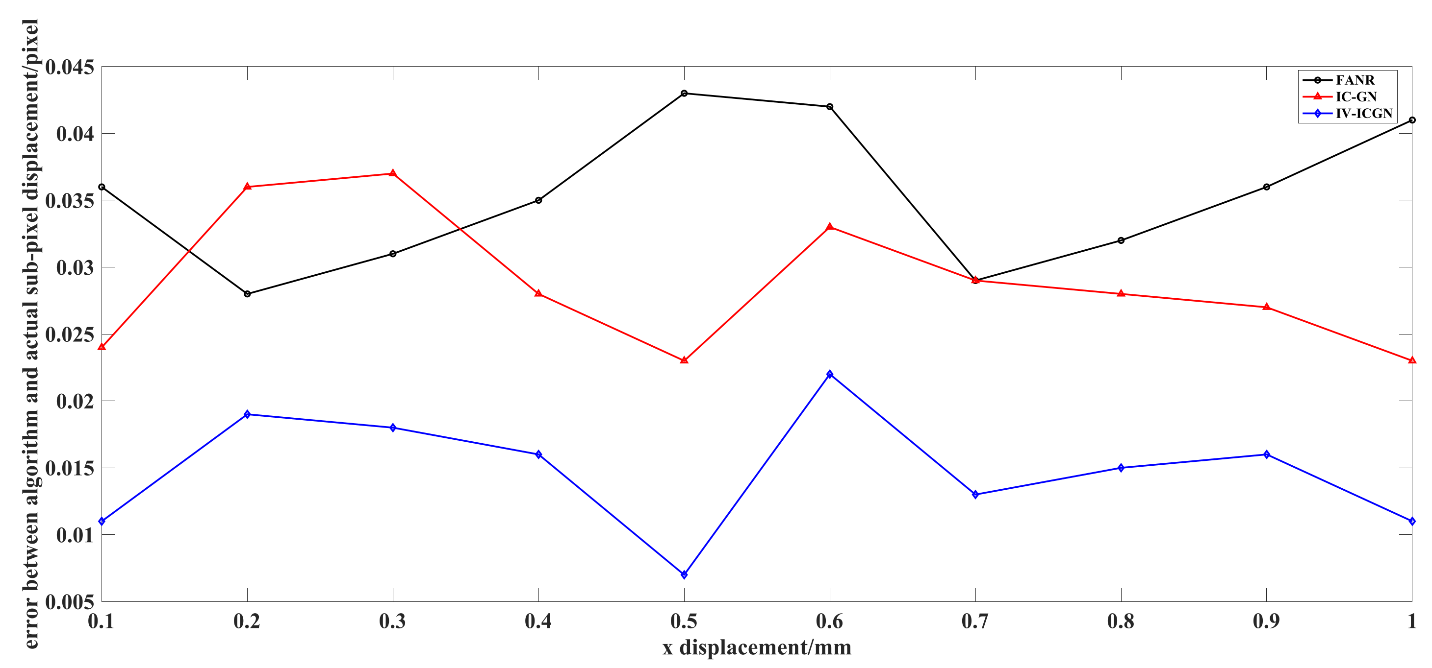
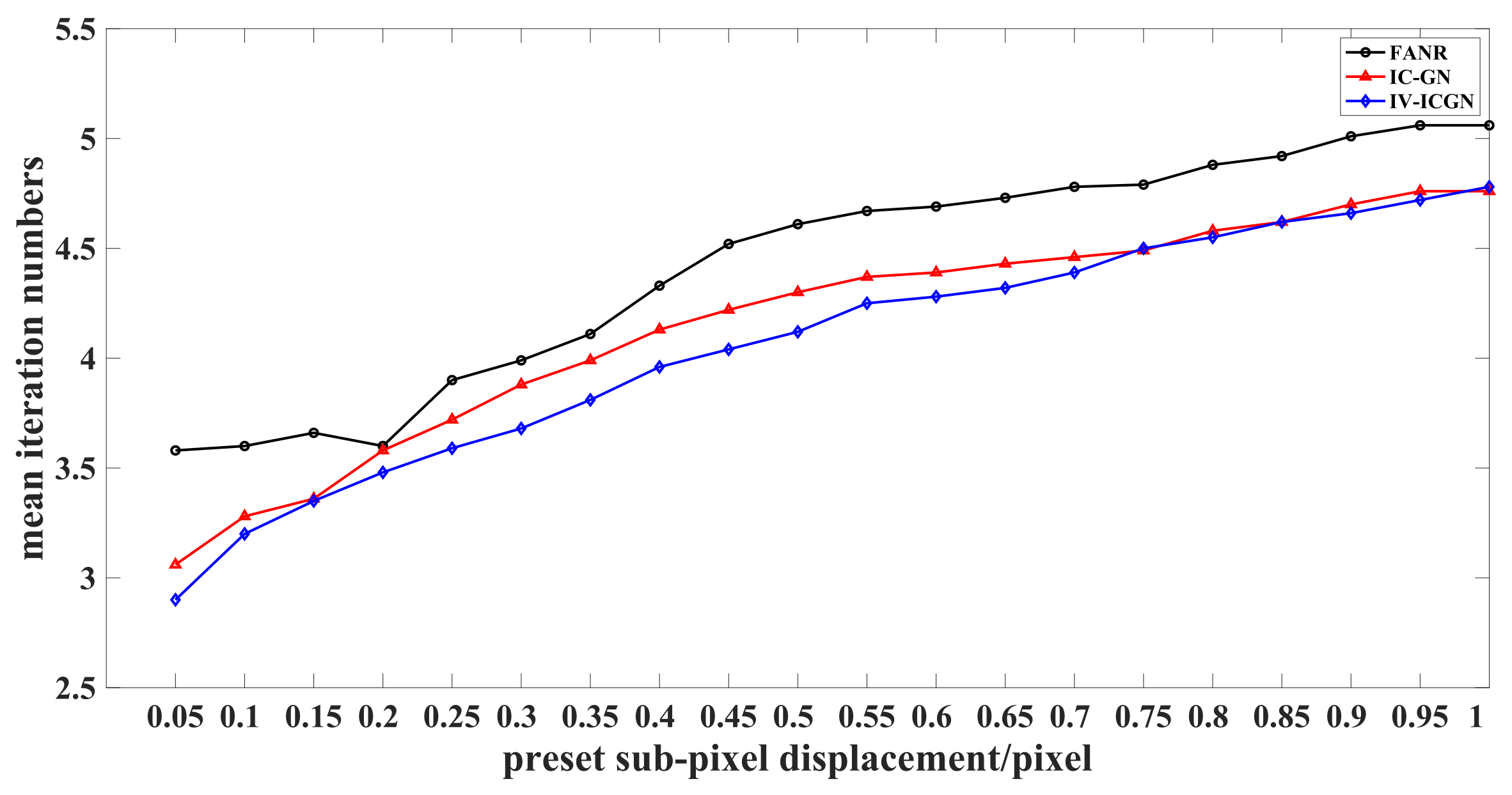
• IV-ICGN algorithm is better than surface fitting, grayscale gradient, FANR and IC-GN algorithms in calculation accuracy and efficiency. The results of simulation experiments show that the mean error value of the IV-ICGN algorithm is smaller than both of the IC-GN and FANR algorithms. In the best case, the mean error of the IV-ICGN algorithm is 66.2% lower than that of the IC-GN algorithm and 69.5% lower than that of the FANR algorithm, the root mean square error of the IV-ICGN algorithm is 15.6% lower than that of the IC-GN algorithm and 17.1% lower than that of the FANR algorithm. In the worst case, the mean error of the IV-ICGN algorithm is 6.0% lower than that of the IC-GN algorithm and 4.6% lower than that of the FANR algorithm, the root mean square error of the IV-ICGN algorithm is 1.4% lower than that of the IC-GN algorithm and 0.3% lower than that of the FANR algorithm. Among the IV-ICGN algorithm, IC-GN algorithm and FANR algorithm, the IV-ICGN algorithm has the least number of iterations.
• Compared with the IC-GN algorithm and FANR algorithm, the accuracy of the IV-ICGN algorithm in real rigid body translation experiments also performs best. The experimental results show that the absolute value of the mean error of the IV-ICGN algorithm is the smallest among the three algorithms, basically between $1\times {10}^{-2}$ pixel and $2\times {10}^{-2}$ pixel, even up to $7\times {10}^{-3}$ pixel. While the other two algorithms are basically between $2\times {10}^{-2}$ pixel and $4\times {10}^{-2}$ pixel.

References

1. Suchorzewski, J.; Prieto, M.; Mueller, U. An experimental study of self-sensing concrete enhanced with multi-wall carbon nanotubes in wedge splitting test and DIC. Constr. Build. Mater. 2020, 262, 120871. [Google Scholar] [CrossRef]
2. Wang, X.; Jin, Z.; Liu, J.; Chen, F.; Feng, P.; Tang, J. Research on internal monitoring of reinforced concrete under accelerated corrosion, using XCT and DIC technology. Constr. Build. Mater. 2021, 266, 121018. [Google Scholar] [CrossRef]
3. Dénes, F.; Gábor, S.; Tamás, T.; Rita, K.M.; Károly, P. Evaluation of the Effect of Freezing and Gamma Irradiation on Different Types of Tendon Allografts by DIC Assisted Tensile Testing. Appl. Sci. 2020, 10, 5369. [Google Scholar]
4. Qiao, X.; Chen, D.; Huo, H.; Tang, M.; Tang, Z.; Dong, Y.; Liu, X.; Fan, Y. Full-field strain mapping for characterization of structure-related variation in corneal biomechanical properties using digital image correlation (DIC) technology. Med. Nov. Technol. Devices 2021, 11, 100086. [Google Scholar] [CrossRef]
5. Ha, N.S.; Jin, T.L.; Goo, N.S. Anisotropy and non-homogeneity of an Allomyrina Dichotoma beetle hind wing membrane. Bioinspiration Biomimetics 2011, 6, 046003. [Google Scholar] [CrossRef]
6. Zhang, H.; Wu, S.; Li, W.; Wang, Y.; Yang, L. Precise Detection of Wrist Pulse Using Digital Speckle Pattern Interferometry. Evid.-Based Complement. Altern. Med. 2018, 2018, 4187349. [Google Scholar] [CrossRef] [Green Version]
7. Polanczyk, A.; Podgorski, M.; Polanczyk, M.; Piechota-Polanczyk, A.; Strzelecki, M. A novel vision-based system for quantitative analysis of abdominal aortic aneurysm deformation. Med. Nov. Technol. Devices 2019, 18, 56. [Google Scholar] [CrossRef] [Green Version]
8. Barile, C.; Casavola, C.; Pappalettera, G. Digital Image Correlation Comparison of Damaged and Undamaged Aeronautical CFRPs During Compression Tests. Materials 2019, 12, 249. [Google Scholar] [CrossRef] [PubMed] [Green Version]
9. Siebert, T.; Hack, E.; Lampeas, G.; Patterson, E.A.; Splitthof, K. Uncertainty Quantification for DIC Displacement Measurements in Industrial Environments. Exp. Tech. 2021, 45, 685–694. [Google Scholar] [CrossRef]
10. Ha, N.S.; Vang, H.M.; Goo, N.S. Modal Analysis Using Digital Image Correlation Technique: An Application to Artificial Wing Mimicking Beetle’s Hind Wing. Exp. Mech. 2015, 55, 989–998. [Google Scholar] [CrossRef]
11. Xie, R.; Chen, G.; Zhao, Y.; Zhang, S.; Yan, W.; Lin, X.; Shi, Q.R.X. In-situ observation and numerical simulation on the transient strain and distortion prediction during additive manufacturing. J. Manuf. Process. 2019, 38, 494–501. [Google Scholar] [CrossRef]
12. Isaac, J.P.; Dondeti, S.; Tippur, H.V. Crack initiation and growth in additively printed ABS: Effect of print architecture studied using DIC. Med. Nov. Technol. Devices 2020, 36, 101536. [Google Scholar] [CrossRef]
13. Stinville, J.C.; Callahan, P.G.; Charpagne, M.A.; Echlin, M.P.; Valle, V.; Pollock, T.M. Direct measurements of slip irreversibility in a nickel-based superalloy using high resolution digital image correlation. Acta Mater. 2020, 186, 172–189. [Google Scholar] [CrossRef]
14. Pan, K.; Yu, R.C.; Ruiz, G.; Zhang, X.; Wu, Z.; De La Rosa, Á. The propagation speed of multiple dynamic cracks in fiber-reinforced cement-based composites measured using DIC. Cem. Concr. Compos. 2021, 122, 104140. [Google Scholar] [CrossRef]
15. Ha, N.S.; Le, V.T.; Goo, N.S. Investigation of fracture properties of a piezoelectric stack actuator using the digital image correlation technique. Int. J. Fatigue 2017, 101, 106–111. [Google Scholar] [CrossRef]
16. Liu, X.; Xiao, Z.; Zhu, R.; Wang, J.; Ma, M. Edge sensing data-imaging conversion scheme of load forecasting in smart grid. Sustain. Cities Soc. 2020, 62, 102363. [Google Scholar] [CrossRef]
17. Kim, K.; Kim, J.S.; Jeong, S.; Park, J.H.; Kim, H.K. Cybersecurity for autonomous vehicles: Review of attacks and defense. Comput. Secur. 2021, 103, 102150. [Google Scholar] [CrossRef]
18. Boukhtache, S.; Abdelouahab, K.; Berry, F.; Blaysat, B.; Grédiac, M.; Sur, F. When Deep Learning Meets Digital Image Correlation. Opt. Lasers Eng. 2021, 136, 106308. [Google Scholar] [CrossRef]
19. Sperry, R.; Han, S.; Chen, Z.; Daly, S.H.; Crimp, M.A.; Fullwood, D.T. Comparison of EBSD, DIC, AFM, and ECCI for active slip system identification in deformed Ti-7Al. Mater. Charact. 2021, 173, 110941. [Google Scholar] [CrossRef]
20. Yang, S.; Chen, M.; Huang, Y.; Jing, H.; Ranjith, P.G. An experimental study on fracture evolution mechanism of a non-persistent jointed rock mass with various anchorage effects by DSCM, AE and X-ray CT observations. Int. J. Rock Mech. Min. Sci. 2020, 134, 104469. [Google Scholar] [CrossRef]
21. Chen, M.; Yang, S.; Ranjith, P.G.; Zhang, Y. Cracking behavior of rock containing non-persistent joints with various joints inclinations. Theor. Appl. Fract. Mech. 2020, 109, 102701. [Google Scholar] [CrossRef]
22. Peters, W.H.; Ranson, W.F. Digital Imaging Techniques In Experimental Stress Analysis. Opt. Eng. 1982, 21, 427–431. [Google Scholar] [CrossRef]
23. Peters, W.H.; Ranson, W.F.; Sutton, M.A.; Chu, T.; Anderson, J. Application Of Digital Correlation Methods To Rigid Body Mechanics. Opt. Eng. 1983, 22, 738–742. [Google Scholar] [CrossRef]
24. Chen, D.; Chiang, F.; Tan, Y.; Don, H. Digital speckle-displacement measurement using a complex spectrum method. Appl. Opt. 1993, 32, 1839. [Google Scholar] [CrossRef] [PubMed]
25. Schreier, H.W.; Sutton, M.A. Systematic errors in digital image correlation due to undermatched subset shape functions. Exp. Mech. 2002, 42, 303–310. [Google Scholar] [CrossRef]
26. Wang, H.; Kang, Y. Improved digital speckle correlation method and its application in fracture analysis of metallic foil. Opt. Eng. 2002, 41, 2793–2798. [Google Scholar] [CrossRef]
27. Rui, J.; Jin, G.; Xu, B. A new digital speckle correlation method and its application. Appl. Mech. 1994, 26, 599–607. [Google Scholar]
28. Liu, G.; Li, M.; Zhang, W. Adaptive Search Algorithm Method of Whole-pixel Deformation for Ancient Building Painted Beams. Hunan Daxue Xuebao/J. Hunan Univ. Nat. Sci. 2020, 47, 106–113. [Google Scholar]
29. Ge, P.; Ye, P.; Li, G. Application of Digital Image Correlation Method Based on Genetic Algorithm in Micro-Displacement Measurement. Guangxue Xuebao/Acta Opt. Sin. 2018, 38, 206–211. [Google Scholar]
30. Zhao, J.; Pan, Z.; Yuan, M.J.Q.Z. Initial guess by improved population-based intelligent algorithms for large inter-frame deformation measurement using digital image correlation. Opt. Lasers Eng. 2012, 50, 473–490. [Google Scholar] [CrossRef]
31. Jiang, Z.; Qian, K.; Hong, M.; Yang, J.; Tang, L. Path-independent digital image correlation with high accuracy, speed and robustness. Opt. Lasers Eng. 2015, 65, 93–102. [Google Scholar] [CrossRef]
32. Zhong, F.; Quan, C. Efficient digital image correlation using gradient orientation. Opt. Laser Technol. 2018, 106, 417–426. [Google Scholar] [CrossRef]
33. Wang, L.; Bi, S.; Lu, X.; Gu, Y.; Zhai, C. Deformation measurement of high-speed rotating drone blades based on digital image correlation combined with ring projection transform and orientation codes. Measurement 2019, 148, 106899. [Google Scholar] [CrossRef]
34. Wu, X.; Yang, Y.; Han, S.; Zhao, Z.; Fang, P.; Gao, Q. Multi-objective optimization method for nuclear reactor radiation shielding design based on PSO algorithm. Ann. Nucl. Energy 2021, 160, 108404. [Google Scholar] [CrossRef]
35. Zhu, W.; Rad, H.N.; Hasanipanah, M. A chaos recurrent ANFIS optimized by PSO to predict ground vibration generated in rock blasting. Appl. Soft Comput. 2021, 108, 107434. [Google Scholar] [CrossRef]
36. Wu, R.; Kong, C.; Zhang, D. Real-Time Digital Image Correlation for Dynamic Strain Measurement. Exp. Mech. 2016, 56, 833–843. [Google Scholar] [CrossRef]
37. Liu, H.; Chen, W.; Xu, Z. An image sub-pixel registration algorithm based on combination of curved surface fitting method and gradient method. Guofang Keji Daxue Xuebao/J. Natl. Univ. Def. Technol. 2015, 37, 180–185. [Google Scholar]
38. ZHou, P.; Goodson, K.E.P.Z. Subpixel displacement and deformation gradient measurement using digital image/speckle correlation (DISC). Opt. Eng. 2001, 40, 1613–1620. [Google Scholar] [CrossRef]
39. Bruck, H.A.; Mcneill, S.R.; Sutton, M.A.; Peters, W.H. Digital image correlation using Newton-Raphson method of partial differential correction. Exp. Mech. 1989, 29, 261–267. [Google Scholar] [CrossRef]
40. Baker, S.; Matthews, I. Equivalence and efficiency of image alignment algorithms. In Proceedings of the 2001 IEEE Computer Society Conference on Computer Vision and Pattern Recognition CVPR 2001, Kauai, HI, USA, 8–14 December 2001. [Google Scholar]
41. Baker, S.; Matthews, I. Lucas-Kanade 20 years on: A unifying framework. Int. J. Comput. Vis. 2004, 56, 221–255. [Google Scholar] [CrossRef]
42. Pan, B.; Li, K.; Tong, W. Fast, robust and accurate digital image correlation calculation without redundant computations. Exp. Mech. 2013, 53, 1277–1289. [Google Scholar] [CrossRef]
43. Li, K.; Cai, P. Study on the performance of sub-pixel algorithm for digital image correlation. Yi Qi Yi Biao Xue Bao/Chin. J. Sci. Instrum. 2020, 41, 180–187. [Google Scholar]
44. Pan, B.; Xie, H.; Dai, F. An investigation of sub-pixel displacements registration algorithms in digital image correlation. Chin. J. Theor. Appl. Mech. 2007, 23, 245–252. [Google Scholar]
45. Schreier, H.; Orteu, J.J.; Sutton, M.A. Image Correlation for Shape, Motion and Deformation Measurements: Basic Concepts, Theory and Applications; Springer Science & Business Media: Boston, MA, USA, 2009. [Google Scholar]
46. Shao, X.; Dai, X.; He, X. Noise robustness and parallel computation of the inverse compositional Gauss–Newton algorithm in digital image correlation. Opt. Lasers Eng. 2015, 71, 9–19. [Google Scholar] [CrossRef]
47. Pan, B.; Wang, B. Digital Image Correlation with Enhanced Accuracy and Efficiency: A Comparison of Two Subpixel Registration Algorithms. Exp. Mech. 2016, 56, 1395–1409. [Google Scholar] [CrossRef]
48. Jiang, L.; Xie, H.; Pan, B. Speeding up digital image correlation computation using the integral image technique. Opt. Lasers Eng. 2015, 65, 117–122. [Google Scholar] [CrossRef]
49. Zhang, L.; Wang, T.; Jiang, Z.; Qian, K.; Liu, Y.; Liu, Z.; Tang, L.; Dong, S. High accuracy digital image correlation powered by GPU-based parallel computing. Opt. Lasers Eng 2015, 69, 7–12. [Google Scholar] [CrossRef]
50. Huang, J.; Zhang, L.; Jiang, Z.; Dong, S.; Chen, W.; Liu, Y.; Liu, Z.; Zhou, L.; Tang, L.Z. Heterogeneous parallel computing accelerated iterative subpixel digital image correlation. Sci. China Technol. Sci. 2017, 61, 74–85. [Google Scholar] [CrossRef] [Green Version]
51. Yang, J.; Huang, J.; Jiang, Z.; Dong, S.; Tang, L.; Liu, Y.; Liu, Z.; Zhou, L. SIFT-aided path-independent digital image correlation accelerated by parallel computing. Opt. Lasers Eng. 2020, 127, 105964. [Google Scholar] [CrossRef]
52. Tong, W. An Evaluation of Digital Image Correlation Criteria for Strain Mapping Applications. Strain 2005, 41, 167–175. [Google Scholar] [CrossRef]
53. Pan, B.; Xie, H.; Wang, Z. Equivalence of digital image correlation criteria for pattern matching. Appl. Opt. 2010, 49, 5501. [Google Scholar] [CrossRef] [PubMed] [Green Version]
54. Fan, J.; Yan, W.; Lei, G. Hierarchical coherency sensitive hashing and interpolation with RANSAC for large displacement optical flow. Comput. Vis. Image Underst. 2018, 175, 1–10. [Google Scholar] [CrossRef]
55. Pan, B.; Lu, Z.; Xie, H. Mean intensity gradient: An effective global parameter for quality assessment of the speckle patterns used in digital image correlation. Opt. Lasers Eng. 2010, 48, 469–477. [Google Scholar] [CrossRef]
56. Jin, T.; Ha, N.S.; Le, V.T.; Goo, N.S.; Jeon, H.C. Thermal buckling measurement of a laminated composite plate under a uniform temperature distribution using the digital image correlation method. Compos. Struct. 2015, 123, 420–429. [Google Scholar] [CrossRef]