Communication

Self-Supervised Deep Learning for Improved Image-Based Wave-Front Sensing

1
Key Laboratory of Optical Engineering, Chinese Academy of Sciences, No. 1 Guangdian Road, Chengdu 610209, China
2
Institute of Optics and Electronics, Chinese Academy of Sciences, Chengdu 610209, China
3
University of Chinese Academy of Sciences, Beijing 100049, China
4
School of Electronic, Electrical and Communication Engineering, University of Chinese Academy of Sciences, Beijing 100049, China
*
Author to whom correspondence should be addressed.
Photonics 2022, 9(3), 165; https://doi.org/10.3390/photonics9030165
Submission received: 7 February 2022 / Revised: 27 February 2022 / Accepted: 4 March 2022 / Published: 9 March 2022

Abstract

:
Phase retrieval from supervised learning neural networks is restricted due to the problem of obtaining labels. To address this situation, in the present paper, we propose a phase retrieval model of self-supervised physical deep learning combined with a complete physical model to represent the image-formation process. The model includes two parts: one is MobileNet V1, which is used to map the input samples to the Zernike coefficients, the other one is an optical imaging system and it is used to obtain the point spread function for training the model. In addition, the loss function is calculated based on the similarity between the input and the output to realize self-supervised learning. The root-mean-square (RMS) of the wave-front error (WFE) between the input and reconstruction is 0.1274 waves in the situation of D/r0 = 20 in the simulation. By comparison, The RMS of WFE is 0.1069 waves when using the label to train the model. This method retrieves numerous wave-front errors in real time in the presence of simulated detector noise without relying on label values. Moreover, this method is more suitable for practical applications and is more robust than supervised learning. We believe that this technology has great applications in free-space optical communication.

1. Introduction

As shown in Figure 1, space light needs to be coupled into single-mode fiber at the receiving end in free-space optical communication (FSOC). However, wave-front aberrations generated by atmospheric turbulence affect the beam quality, then deteriorate the fiber coupling efficiency and the quality of communication. Therefore, it is necessary to detect and correct the wave-front aberration. The measurement of the wave-front aberration in FSOC differs from other scenarios in that the wave-front aberration changes continuously. Therefore, an accurate real-time measurement is required in FSOC. There are two main methods for measuring wave-front aberrations. The first method uses additional wave-front sensors, such as a Hartmann sensor or interferometer [1,2,3], to monitor the wave-front slope. The other method uses the spot quality as the objective function and optimizes the objective function with continuous iteration, such as an image-based sensor [4,5,6,7]. The real-time performance of this second method is poor, so its application range is very limited. Deep learning is applied to the image-based sensor in order to improve the real-time performance of this method.
Image-based wave-front sensing uses parametric physical models and a measured point spread function (PSF) with nonlinear optimization for calculation [8,9,10]. Artificial neural networks are nonlinear, autonomous, and regulated information-processing systems for learning and generalized nonlinear mapping between inputs and outputs [11,12,13]. At the end of the twentieth century, artificial neural networks were used to measure the optical phase distortion caused by atmospheric disturbance [14,15,16], although the structure of the neural networks in the system was too simple at that time, resulting in poor generalization. Since then, significant research has optimized the neural network structure.
Convolutional neural networks (CNNs) [17,18,19] use convolutional kernels and down-sampling to perform machine-learning tasks on images, which reduces the dimensionality of large data volumes and retains image features. In another approach, Paine et al. used Inception V3 for phase detection [20], but the PSFs used in the training set were set at the focal point with less effective information, which led to fitting error. Nishizaki proposed the generalized wave-front sensing framework [21] to estimate a single intensity distribution and showed that the proper preprocessing of a single intensity image improves the calculation and fitting accuracy.
Compared to the output of CNNs is the class label of the entire image, UNet is a pixel-level classification that outputs the pixel category and is often used on biomedical images [22,23]. Given that image data in this task are often small, Ciresan et al. trained a CNN using a sliding window to provide the pixel and its surroundings as input to predict the class label of each pixel. UNets are also widely used in the wave-front detection field [24,25,26], but the network structure is complex and too slow for real-time tasks.
To summarize, conventional supervised learning neural networks have good detection accuracy, but the many labeled data samples for training greatly increase application costs and difficulty. The essence of this approach is to map PSF image pixels to Zernike coefficients. UNet uses data enhancement to solve the problem of few training images, but it cannot extract the control parameters required for phase correction, such as Zernike coefficients.
Unsupervised learning uses pretexts to mine its own supervised information from large-scale unsupervised data and learns valuable representations for downstream tasks. In another approach, Wang proposed phase imaging with an untrained neural network [27] to iterate over a single damaged image, learn the prior information on the image, and restore the image. However, when the important features of an image are damaged, the image is not easily repaired. Because training in advance is not possible, every time the image is processed, it must be iterated many times to achieve an ideal result. Emrah Bostan proposed using an untrained neural network to restore the phase without a label [28]. Poor generalization is the same problem as above, because offline processing does not require high real-time performance. However, high real-time performance is important in the measurement of wave-front aberration in free-space optical communication. Ramos [29] proposed the use of blind convolution to restore multiple targets, but the network structure is complex, the calculation time is long, and the accuracy is poor. Tobias Liaudat proposed a paradigm shift in the data-driven modeling of the instrumental response field of telescopes by adding a differentiable optical forward model into the modeling framework [30]. This approach is also an unsupervised training based on optical modeling, but the aim is to simplify the building of the instrumental response model.
To solve these problems, we propose a phase retrieval method based on self-supervised physical deep learning (PDL), which maps the input data to hidden vectors through a deep neural network and combines the optical imaging physical model to fit the output. In addition, a retrieval model is established according to the mapping relationship between input and output. Compared with traditional CNNs, this method does not rely on labels, but only establishes the relationship between the collected light spot samples through the intrinsic characteristics of the PSF. Compared with UNet, the Zernike coefficient is more quickly extracted, giving this method better real-time performance. This method also avoids the technical bottleneck of traditional supervised learning that requires many label samples, which facilitates practical applications. Compared with the existing self-supervised learning network, the reasoning for new information requires only one step and the accuracy is higher, but the method we proposed can only be applied to the detection of point objects.

2. Method

As shown in Figure 2, PDL includes three parts: network encoding, a hidden layer vector, and network decoding.

2.1. Encoding Part

The encoder maps the input samples to the hidden layer vector. We tested the ImageNet classification CNN and chose MobileNet [31], which is more suitable for mobile terminals. MobileNet consists of a 3 × 3 standard convolution, followed by a stacked depth-wise separable convolution, some of which involves down-sampling through strides = 2. Average pooling is used to change the feature to 1 × 1, and a fully connected layer is added according to the predicted category size. The batch size is 32. Since we are not dealing with a classification problem, we removed the last SoftMax layer. The core consists of a decomposable depth-wise separable convolution, which not only reduces the computational complexity of the model, but also reduces the size of the model.
For real mobile application scenarios that require low latency, networks, such as MobileNet, are the focus of continuous research. Depth-wise separable convolution is a factorized convolution operation that can be decomposed into two smaller operations: depth-wise convolution and pointwise convolution. Depth-wise convolution uses a different convolution kernel for each input channel and pointwise convolution uses a 1 × 1 convolution kernel. The former uses depth-wise convolution to separately convolve different input channels and then uses pointwise convolution to combine the above outputs.

2.2. Decoding Part

The model of optical imaging system is shown in Figure 3 and it is the decoding part in the network. The object plane is regarded as the weighted superposition of primitive objects according to the imaging principle of convolution. For the image plane, this is the coherent superposition of the diffraction image produced by the corresponding object point [32]. The relationship between the image plane and the object plane can be expressed as the following convolution:
g i ( x , y ) = g o ( x 0 , y 0 ) h ( x , y ) ,
where g i ( x , y ) is the complex optical amplitude distribution of the image plane; g o ( x 0 , y 0 ) is the complex optical amplitude of the object plane under ideal conditions; x and y are in the image plane and x 0 and y 0 are in the object plane; ∗ is the convolution operator; and h is the impulse response function of the system, also called the PSF, which is used to describe the two-dimensional distribution of light on the focal plane from a point-source imaging system. For a point target, this is equivalent to a linear space-invariant incoherent imaging system. The object and image plane functions satisfy the linear transformation of intensity:
I i ( x , y ) = I o ( u , v ) h ( x u , v y ) d u d v ,
where I i is the intensity distribution system at the image plane; I o is the ideal intensity distribution system at the object plane; and u and v are the coordinates of the pupil plane. In the case of point targets, the object–image relation of the system and the PSF in the case of the diffraction limitation is expressed as
g i ( x , y ) = h ( x , y ) = | FFT { P ( u , v ) } | 2 ,
where FFT is the fast Fourier transform operator and P is the generalized pupil function. In the case of aberration, the pupil function on the image plane at the exit-pupil position is expressed as
P ( u , v ) = O ( u , v ) e 2 π i ϕ ( u , v ) ,
where O ( u , v ) is the aperture function; the value inside the aperture is unity; the value outside the aperture is zero; and ϕ ( u , v ) is the phase-distribution function at the pupil plane. The Zernike mode method makes use of a set of polynomials that reflect the orthogonal properties of a circular region. Therefore, the Zernike mode method is usually used as an orthogonal basis for wave-front reconstruction. Wave-front phase functions (x, y) in the circular domain can be expanded into Zernike polynomials as follows:
φ ( x , y ) = i = 1 i = a i z i ( x , y ) ,
where a i is the coefficient of the pattern of term i and z i is the Zernike pattern corresponding to term i. The matrix distribution of the Zernike coefficient is composed of the all-order polynomials and the corresponding coefficients:
Z i ( r , θ ) = { N n m R n | m | ( r ) cos ( m θ ) ,   m 0 N n m R n | m | ( r ) sin ( m θ ) ,   m 0 ,
where 0 r 1 , 0 θ 2 π ; n is a non-negative integer; the step length m = 2; the outputs are between −n and n; and R n | m | is the radial function for the polynomials. The hidden layer vector we used in the network is a Zernike coefficient. The aberration can be calculated with the Zernike coefficients and polynomials. Then, the PSF can be obtained by the optical imaging system for training the model.

2.3. Loss Function

We strived to make the inputs and outputs of the network consistent by using the correlation coefficient between the input and output PSF as a loss function. The formula for calculating the correlation coefficients is
r = m n ( A m n A ¯ ) ( B m n B ¯ ) ( m n ( A m n A ¯ ) 2 ) ( m n ( B m n B ¯ ) 2 ) ,
where A and B are the pixel values of the two PSFs, and A ¯ and B ¯ are the mean values of A and B, respectively. When the model training is completed, the model interferes without the decoding part. The output of the network is a Zernike coefficient and can be used to correct aberrations. Therefore, there is no difference in the resource consumption and time consumption, compared to the supervised networks.

3. Simulation Demonstration

3.1. Simulation Demonstration of 3–20 Orders of Zernike Polynomials

The simulation data set is generated by using the Zernike pattern method. The piston error (The Zernike polynomial Z 0 ) is ignored because it is the translation of the beam phase and does not affect the beam quality. The tip and tilt terms ( Z 1 and Z 2 ), which can be quickly estimated by using the centroid algorithm or other registration methods, are also ignored. The PSF simulation model in this article sets the pupil size to 8.6 mm, the focal length of the lens to 150 mm, and the defocus to 8 mm. The wavelength of the optical source is 532 nm, and to simulate the actual environment, Gaussian white noise with a mean value of 0 and a variance of 0.01 is added to the PSF. In the case of different mode coefficients, 22,000 distorted spot images are generated with D/r0 = 20, 20,000 out-of-focus PSFs are input into the self-supervised learning neural network, and PDL is applied according to the correlation coefficient between the input and output PSFs. A total of 2000 PSFs were tested, and the Zernike coefficients were inferred on the basis of the mapping relationship.
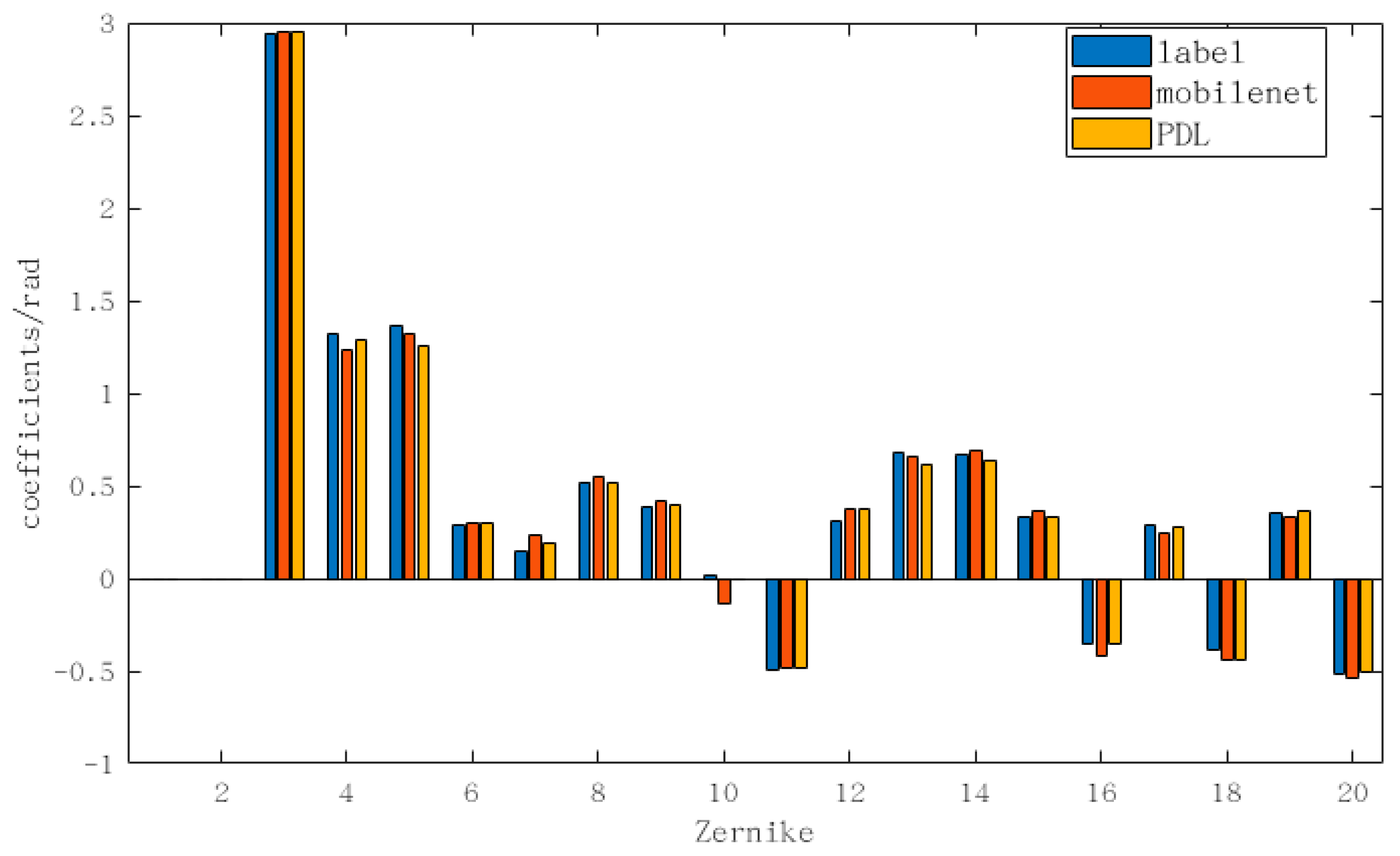
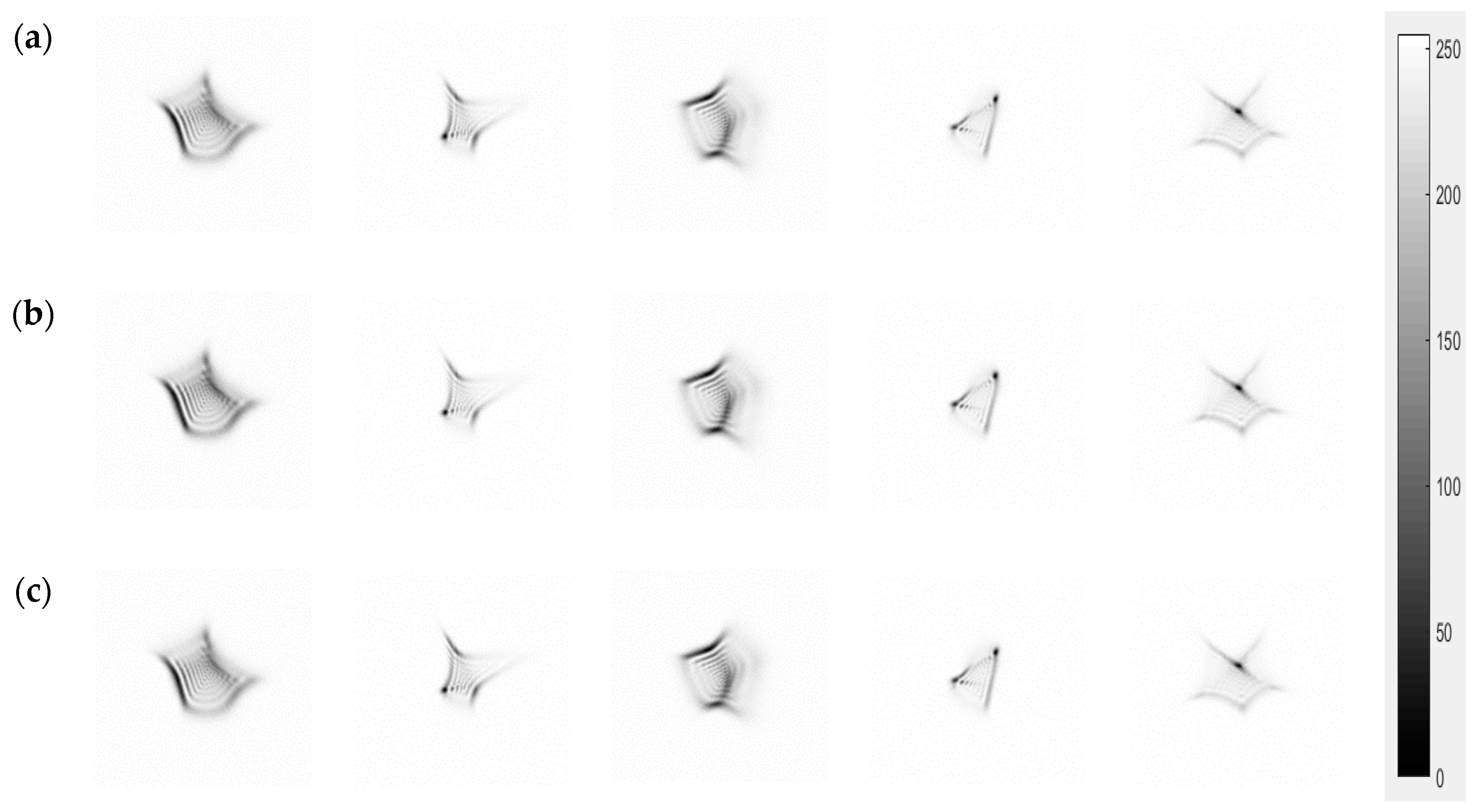
Figure 4 and Figure 5 shows the test results, and the PSF images are normalized. The image size is 256 × 256 and the pixel size is 5.5 µm. Moreover, Table 1 lists the root mean square errors (RMSEs) obtained from testing and inference. To reflect the retrieval effect of PDL more clearly, we compared the results with those of the MobileNet supervised learning method. For coefficients 3–20, the RMSE of the original distortion wave-front is 0.8284λ. The correlation coefficient of the test set was 97%, and the RMSE of the one-time calibration is 0.0648λ. In contrast, the supervised corrected wave-plane RMSE is 0.0447λ. Although the detection accuracy is slightly lower compared with supervised learning, no a priori knowledge of the Zernike coefficients is required, which facilitates practical applications.
To test the generalization ability of the network, 3000 distorted spot images are generated with D/r0 interval 5 from 5 to 30. The network trained before is used to inference the 3000 distorted spot images. Table 2 shows the results. The results show that the generalization ability of the network is good.

3.2. Simulation Demonstration of 3–64 Orders of Zernike Polynomials

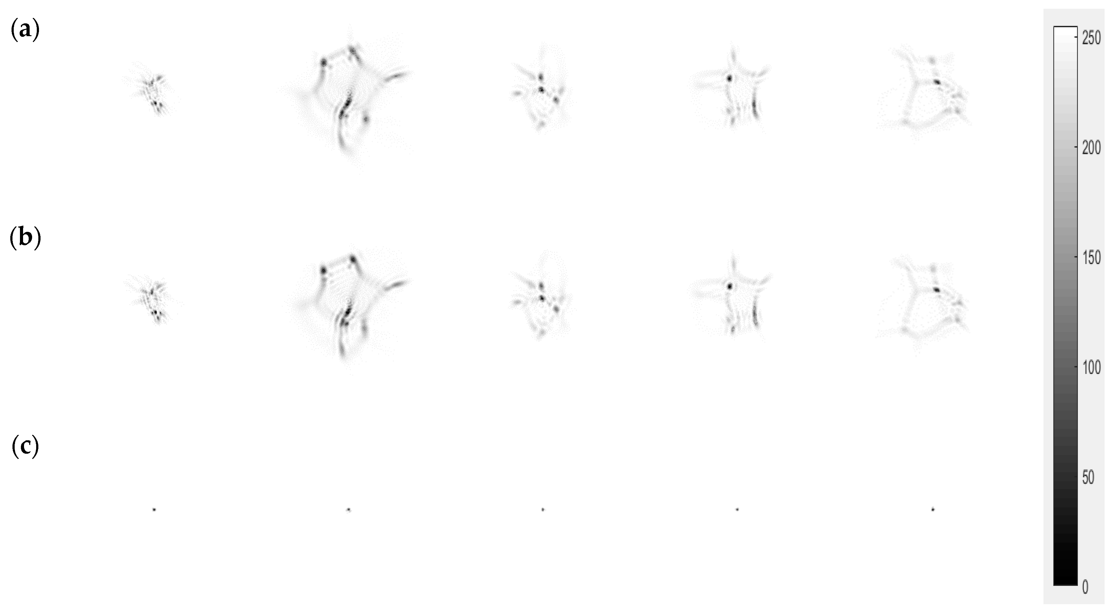
The influence of higher-order wave-front aberrations on the network performance is considered as follows: the 3–64 Zernike order is used to train the network; the RMSE of the original distortion wave-front is 0.8852λ; and the corrected wave front RMSE of PDL is 0.1274λ and the RMSE of MobileNet is 0.1069λ. Figure 6, Table 3 and Table 4 shows the test results, and the PSF images are normalized. The image size is 256 × 256 and the pixel size is 5.5 µm. The results show that the performance of the self-supervised network is also close to the supervised network in the high-order case.

4. Experimental Demonstration

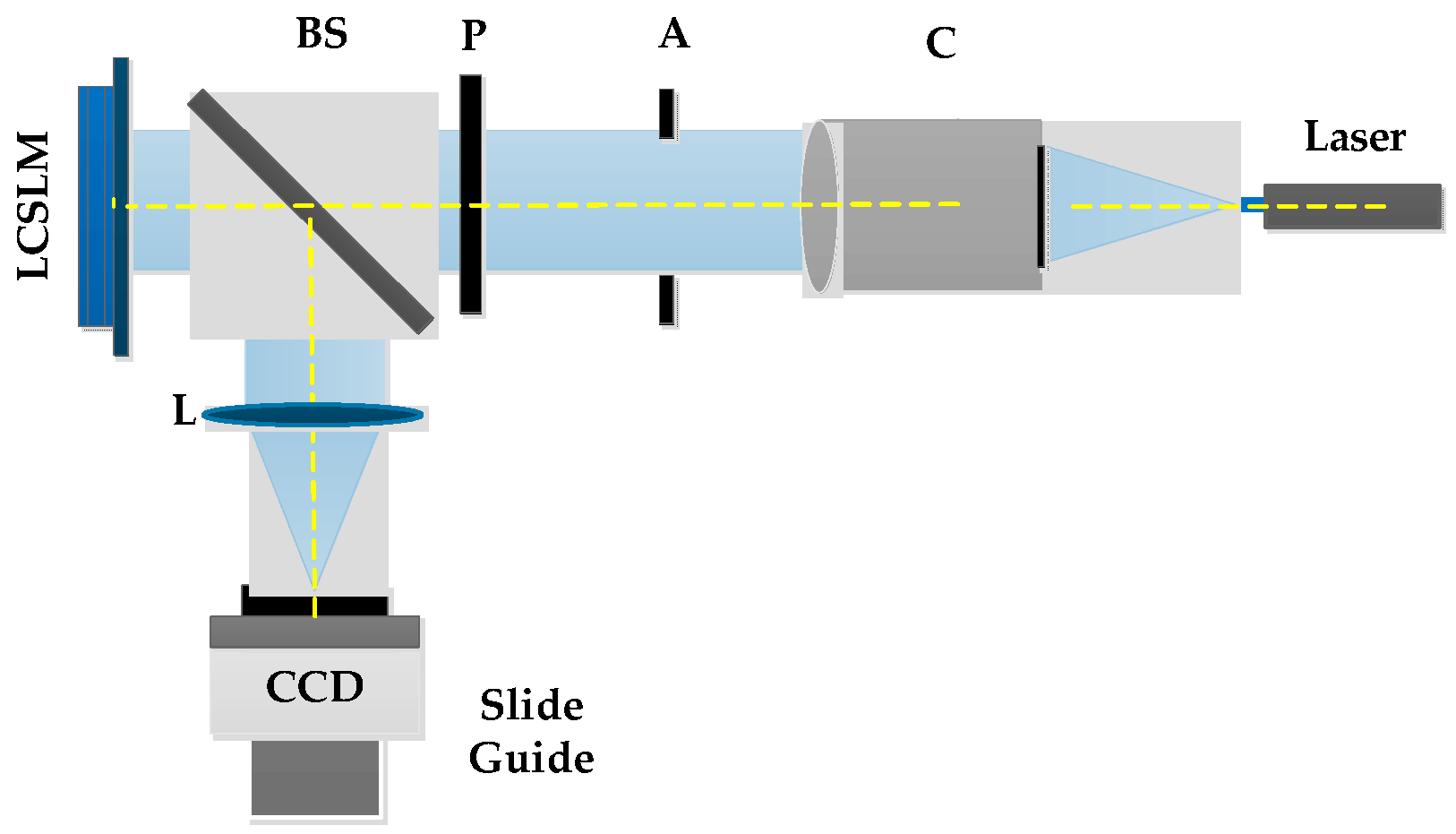
Figure 7 shows the optical platform of the phase retrieval experiment, which used a liquid crystal spatial light modulator (LCSLM) to simulate the PSF. A 532 nm laser served as a light source. A collimator expanded the beam, which was normal to the incident aperture (A), polarizer (P), and the LCSLM. The size of the aperture was limited to 8.6 mm to ensure that the incident light was evenly distributed over the center of the LCSLM. The BS changed the direction of the light beam modulated by the LCSLM. Phase distortion was simulated by loading different grayscale phase screens onto the LCSLM. Due to a small gap between the pixels, higher diffraction orders and a high-energy zero-order spot exist at the output. An X tilt was added to displace the spot from the central zero-order spot. The modulated light was imaged through the lens (L) before impinging on the CCD. The effective resolution of the CCD acquisition window was 256 × 256, which was compressed to 128 × 128 for training and testing. To ensure the detection accuracy of the neural network and the range of the CCD field of view, we set the CCD defocus to 8 mm. To ensure clear imaging with the CCD, a suitable attenuator was positioned in front of the CCD. The model pluto-2-NIR-011LCSLM used in this experiment was produced by HoloEye and has a pixel resolution of 1920 × 1080, with 8 µm pixels. As with the simulations, we trained with 20,000 experimental images and tested with 2000 PSFs. The overall tilt of the experiment used the Zernike coefficients of order 1–20 to produce a test set correlation coefficient of 95%. Figure 8 shows the calculation results obtained by inputting the collected light spot into the experimental training model. The image size is 256 × 256 and the pixel size is 5.5 µm. The light spots are similarly shaped. A Jetson TX2 from NVIDIA was used for inference calculations. After using tensor optimization on the TX2, the single-inference time is 3.72 ms, which is adequate for real-time performance.

5. Discussion

The experimental results are the same as we expected. The detection accuracy of the self-supervised deep learning model proposed in this paper is slightly inferior to the supervised deep learning model. However, the self-supervised model reduces the difficulty of sample acquisition, so it is easier to apply in practice. The supervised model is related to the method proposed in reference [22]. We made some adjustments to the method, according to the new application scenario. Due to the change of atmosphere turbulence intensity, the result of the supervised model is different from those in reference [22].
Compared to other self-supervised models based on the optical imaging system mentioned in the Introduction, we proposed a new network model. Additionally, a new loss function, the correlation coefficient, was used to train the network with batch-size in practice. Training with batch-size presents our network with a high detection accuracy and good generalization ability.
However, the training of the method needs to know the optical parameters, such as optical aperture, the focal length of lens, etc. In most application scenarios, these parameters are known.

6. Conclusions

Herein, we proposed a self-supervised model that retrieves the phase without labels. The model is generalizable, can be used with different networks, and can solve different problems. In addition, for reasoning, it does not affect the time consumption of the network. The model is suitable for practical applications of deep learning for phase detection and other optical problems. Although the detection accuracy is slightly less than that provided by supervised learning, no a priori knowledge of the Zernike coefficients is required, which facilitates practical applications.
In future work, we will validate the effectiveness of PDL in satellite-to-ground laser communication. Additionally, we will use different loss functions and train them to estimate other terms. PDL will be adapted to different wavelengths, apertures, and focal lengths, in order to directly measure spots of different wavelengths, apertures, and focal lengths without retraining or changing the models.

Author Contributions

Conceptualization, Y.X.; methodology, Y.X.; software, Y.X.; validation, Y.X., H.G. and Z.W.; formal analysis, Y.X.; investigation, Y.X.; resources, D.H.; data curation, Z.W.; writing—original draft preparation, Y.X. and H.G.; writing—review and editing, Y.X., H.G. and D.H.; visualization, Z.W.; supervision, Y.H.; project administration, Y.H.; funding acquisition, Y.T. and Y.H. All authors have read and agreed to the published version of the manuscript.

Funding

The National Key Research and Development Program of China (2017YFB11030002).

Institutional Review Board Statement

This study did not involve humans or animals.

Informed Consent Statement

Not applicable.

Data Availability Statement

Data underlying the results presented in this paper are not publicly available at this time, but may be obtained from the authors upon reasonable request.

Conflicts of Interest

The authors declare no conflict of interest.

References

  1. Platt, B.C.; Shack, R. History and principles of Shack-Hartmann wavefront sensing. J. Refract. Surg. 1995, 17, 573–577. [Google Scholar] [CrossRef] [PubMed]
  2. Vargas, J.; González-Fernandez, L.; Quiroga, J.A.; Belenguer, T. Calibration of a Shack-Hartmann wavefront sensor as an orthographic camera. Opt. Lett. 2010, 35, 1762–1764. [Google Scholar] [CrossRef] [PubMed] [Green Version]
  3. Gonsalves, R.A. Phase retrieval and diversity in adaptive optics. Opt. Eng. 1982, 21, 829–832. [Google Scholar] [CrossRef]
  4. Nugent, K.A. The measurement of phase through the propagation of intensity: An introduction. Contemp. Phys. 2011, 52, 55–69. [Google Scholar] [CrossRef]
  5. Misell, D.L. An examination of an iterative method for the solution of the phase problem in optics and electronoptics: I. Test calculations. J. Phys. D Appl. Phys. 1973, 6, 2200–2216. [Google Scholar] [CrossRef]
  6. Fienup, J.R. Phase-retrieval algorithms for a complicated optical system. Appl. Opt. 1993, 32, 1737–1746. [Google Scholar] [CrossRef]
  7. Allen, L.J.; Oxley, M.P. Phase retrieval from series of images obtained by defocus variation. Opt. Commun. 2001, 199, 65–75. [Google Scholar] [CrossRef]
  8. Carrano, C.J.; Olivier, S.S.; Brase, J.M.; Macintosh, B.A.; An, J.R. Phase retrieval techniques for adaptive optics. Adapt. Opt. Syst. Technol. 1998, 3353, 658–667. [Google Scholar]
  9. Gerchberg, R.W.; Saxton, W.O. A practical algorithm for the determination of phase from image and diffraction plane pictures. Optik 1972, 35, 237–246. [Google Scholar]
  10. Yang, G.Z.; Dong, B.Z.; Gu, B.Y.; Zhuang, J.Y.; Ersoy, O.K. Gerchberg–Saxton and Yang–Gu algorithms for phase retrieval in a nonunitary transform system: A comparison. Appl. Opt. 1994, 33, 209–218. [Google Scholar] [CrossRef]
  11. Hagan, M.T.; Beale, M. Neural Network Design; China Machine Press: Beijing, China, 2002. [Google Scholar]
  12. Mello, A.T.; Kanaan, A.; Guzman, D.; Guesalaga, A. Artificial neural networks for centroiding elongated spots in Shack-Hartmann wave-front sensors. Mon. Not. R. Astron. Soc. 2014, 440, 2781–2790. [Google Scholar] [CrossRef] [Green Version]
  13. Guo, H.J.; Xin, Q.; Hong, C.M.; Chang, X.Y. Feature-based phase retrieval wave front sensing approach using machine learning. Opt. Express 2018, 26. [Google Scholar]
  14. Fienup, J.R.; Marron, J.C.; Schulz, T.J.; Seldin, J.H. Hubble Space Telescope characterized by using phase-retrieval algorithms. Appl. Opt. 1993, 32, 1747–1767. [Google Scholar] [CrossRef] [PubMed] [Green Version]
  15. Roddier, C.; Roddier, F. Wave-front reconstruction from defocused images and the testing of ground-based optical telescopes. J. Opt. Soc. Am. A 1993, 10, 2277–2287. [Google Scholar] [CrossRef]
  16. Redding, D.; Dumont, P.; Yu, J. Hubble Space Telescope prescription retrieval. Appl. Opt. 1993, 32, 1728–1736. [Google Scholar] [CrossRef]
  17. Shin, H.C.; Roth, H.R.; Gao, M.; Lu, L.; Xu, Z.; Nogues, I.; Yao, J.; Mollura, D.; Summers, R.M. Deep convolutional neural networks for computer-aided detection: CNN architectures, dataset characteristics and transfer learning. IEEE Trans. Med. Imaging 2016, 35, 1285–1298. [Google Scholar] [CrossRef] [Green Version]
  18. Goodfellow, I.; Bengio, Y.; Courville, A. Learning D[M]; MIT Press: Cambridge, MA, USA, 2016. [Google Scholar]
  19. Gu, J.; Wang, Z.; Kuen, J.; Ma, L.; Shahroudy, A.; Shuai, B.; Liu, T.; Wang, X.; Wang, G.; Cai, J.; et al. Recent advances in convolutional neural networks. Pattern Recognit. 2018, 77, 354–377. [Google Scholar] [CrossRef] [Green Version]
  20. Paine, S.W.; Fienup, J.R. Machine learning for improved image-based wavefront sensing. Opt. Lett. 2018, 43, 1235–1238. [Google Scholar] [CrossRef]
  21. Nishizaki, Y.; Valdivia, M.; Horisaki, R. Deep learning wave front sensing. Opt. Express 2019, 27, 240–251. [Google Scholar] [CrossRef]
  22. Long, J.; Shelhamer, E.; Darrell, T. Fully convolutional networks for semantic segmentation. IEEE Trans. Pattern Anal. Mach. Intell. 2017, 39, 640–651. [Google Scholar]
  23. Ronneberger, O.; Fischer, P.; Brox, T. U-net: Convolutional networks for biomedical image segmentation. arXiv 2015, arXiv:1505.04597. [Google Scholar]
  24. Swanson, R.; Lamb, M.; Correia, C.; Sivanandam, S.; Kutulakos, K. Wave-front reconstruction and prediction with convolutional neural networks. Adapt. Opt. Syst. VI 2018, 10703, 107031F. [Google Scholar]
  25. Dubose, T.B.; Gardner, D.F.; Watnik, A.T. Intensity-enhanced deep network wave-front reconstruction in Shack Hartmann sensors. Opt. Lett. 2020, 45, 1699–1702. [Google Scholar] [CrossRef]
  26. Hu, L.J.; Hu, S.W.; Gong, W.; Si, K. Deep learning assisted Shack-Hartmann wave-front sensor for direct wave-front detection. Opt. Lett. 2020, 45, 3741–3744. [Google Scholar] [CrossRef] [PubMed]
  27. Fei, W.; Bian, Y.; Wang, H.; Lyu, M.; Pedrini, G.; Osten, W.; Barbastathis, G.; Situ, G. Phase imaging with an untrained neural network. Light Sci. Appl. 2020, 9, 77. [Google Scholar]
  28. Bostan, E.; Heckel, R.; Chen, M.; Kellman, M.; Waller, L. Deep phase decoder: Self-calibrating phase microscopy with an untrained deep neural network. Optica 2020, 7, 559. [Google Scholar] [CrossRef] [Green Version]
  29. Ramos, A.A.; Olspert, N. Learning to do multiframe wave front sensing unsupervised: Applications to blind deconvolution. Astron. Astrophys. 2021, 646, A100. [Google Scholar] [CrossRef]
  30. Liaudat, T.; Starck, J.; Kilbinger, M.; Frugier, P. Rethinking the modeling of the instrumental response of telescopes with a differentiable optical model. arXiv 2021, arXiv:2111.12541. [Google Scholar]
  31. Howard, A.G.; Zhu, M.; Chen, B.; Kalenichenko, D.; Wang, W.; Weyand, T.; Andreetto, M.; Adam, H. MobileNets: Efficient convolutional neural networks for mobile vision applications. arXiv 2017, arXiv:1704.04861. [Google Scholar]
  32. Wen, Z. Photon Foundation; Zhejiang University Press: Hangzhou, China, 2000. [Google Scholar]
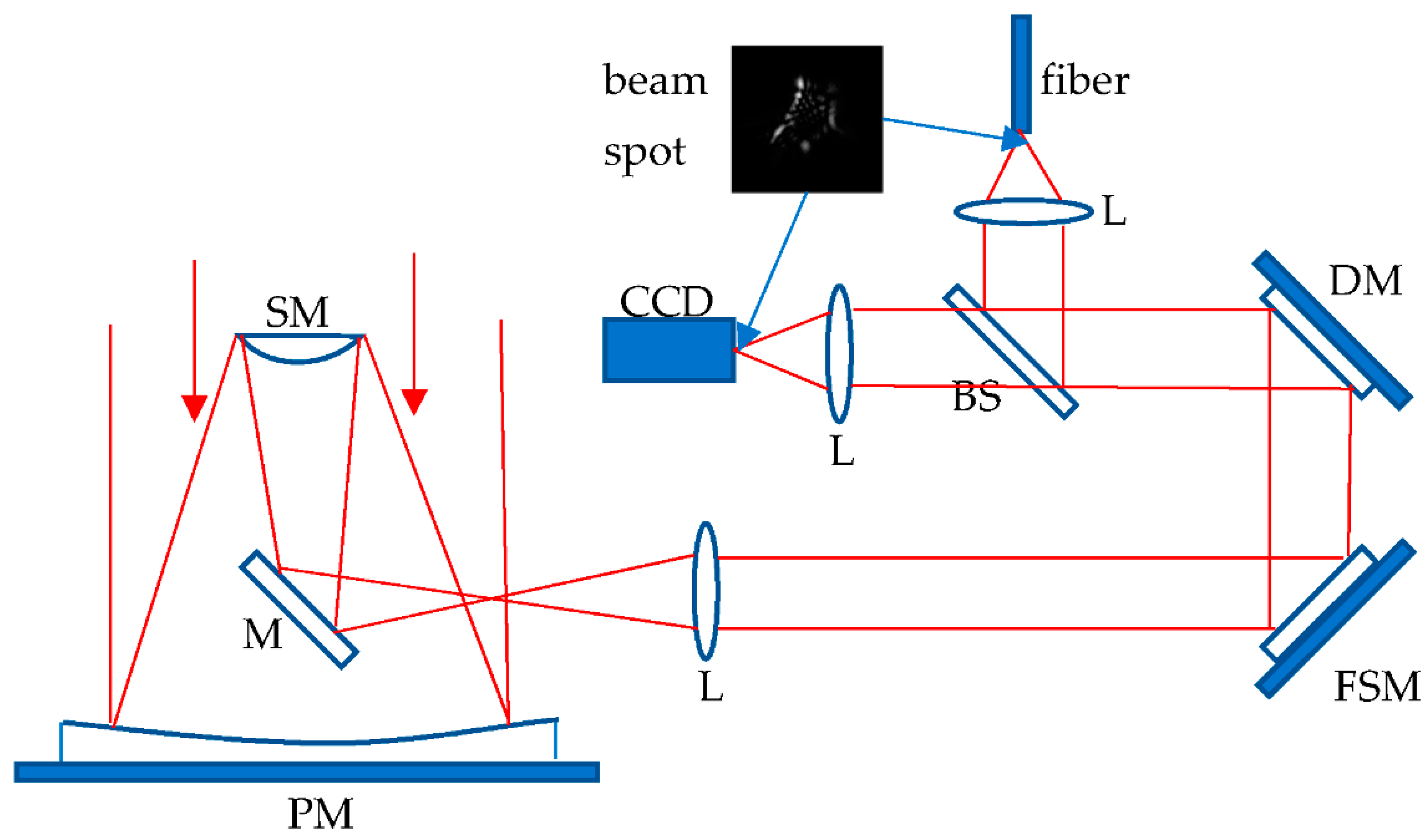
Figure 1. Schematic diagram of fiber coupling based on an image sensor in free-space optical communication. PM: primary mirror; SM: secondary mirror; M = mirror; BS = beam splitter; FSM = fast steering mirror; DM = deformable mirror; L = lens; and CCD = charge-coupled device.
Photonics 09 00165 g001
Figure 2. Structure diagram of the self-supervised learning neural network model.
Photonics 09 00165 g002
Figure 3. The model of optical imaging system.
Photonics 09 00165 g003
Figure 4. Comparison of the Zernike coefficient between original distributions, supervised learning, and self-supervised learning.
Photonics 09 00165 g004
Figure 5. Comparison of the PSF image with 3–20 orders of Zernike polynomials (intensity reversed): (a) original distribution, (b) supervised learning recovery spots, and (c) self-supervised learning recovery spots. (The pixel size is 5.5 µm and the image size is 256 × 256).
Photonics 09 00165 g005
Figure 6. Comparison of the PSF image with 3–64 orders of Zernike polynomials (intensity reversed): (a) original distribution, (b) self-supervised learning recovery spots, and (c) the correction spot. (The pixel size is 5.5 µm and the image size is 256 × 256).
Photonics 09 00165 g006
Figure 7. Experimental diagram of the physical deep learning wave-front sensor. C = collimator; A = aperture; P = polarizer; BS = beam splitter; LCSLM = liquid crystal spatial light modulator; and L = lens; CCD = charge-coupled device.
Photonics 09 00165 g007
Figure 8. Experimentally acquired PSF compared with the PDL recovery with Zernike coefficients 4–20 (intensity reversed). (a) PSF collected experimentally; (b) simulation PSF; and (c) restored PSF by simulation. (The pixel size is 5.5 µm and the image size is 256 × 256).
Photonics 09 00165 g008
Table 1. Comparison of accuracies (RMSE) of equivalent wave-fronts from the Zernike coefficients estimated in the experiments between PDL and MobileNet (3–20 orders).
Zernike OrderRMSE of Testing SetRMSE of MobileNetRMSE of PDL
3–200.8284λ0.0447λ0.0648λ
Table 2. Comparison of the accuracies (RMSE) of the equivalent wave-fronts from the Zernike coefficients estimated in the experiments between PDL and MobileNet with different D/r0 (3–20 order).
D/r0RMSE of Testing SetRMSE of MobileNetRMSE of PDL
301.1991λ0.1176λ0.1469λ
250.9962λ0.0621λ0.0762λ
200.8606λ0.0462λ0.0634λ
150.6651λ0.0396λ0.0519λ
100.4641λ0.0276λ0.0352λ
50.2615λ0.0232λ0.0256λ
Table 3. Comparison of accuracies (RMSE) of equivalent wave-fronts from the Zernike coefficients estimated in the experiments between PDL and MobileNet (3–64 orders).
Zernike OrderRMSE of Testing SetRMSE of MobileNetRMSE of PDL
3–640.8852λ0.1069λ0.1274λ
Table 4. Comparison of the accuracies (RMSE) of the equivalent wave-fronts from the Zernike coefficients estimated in the experiments between PDL and MobileNet with different D/r0 (3–64 orders).
D/r0RMSE of Testing SetRMSE of MobileNetRMSE of PDL
301.2021λ0.3052λ0.3487λ
251.0438λ0.1887λ0.2136λ
200.8784λ0.1084λ0.1255λ
150.676λ0.0857λ0.0984λ
100.4864λ0.0671λ0.0696λ
50.2715λ0.0610λ0.0611λ
Publisher’s Note: MDPI stays neutral with regard to jurisdictional claims in published maps and institutional affiliations.