Abstract
Holographic optical storage has great potential for enormous data storage, although the recording medium can cause dimensional change, which can deteriorate the quality of the reconstructed hologram. Compensation in traditional off-axial holographic storage systems is sensitive to vibration and requires high precision. In contrast, a collinear system is more compact with better stability, and its compensation would be different. In this paper, the combination compensation method for compensating for the dimensional change of the recording medium by simultaneously adjusting the reading light wavelength and the focal length of the objective lens is established, which was implemented in a collinear system for a high dimension-change-rate (σ) of the medium condition. Its compensation effects for the lateral dimension change and the vertical dimension change were compared as well. The results show that the bit error ratio of the reconstructed hologram could be decreased to 0 for both of the dimensional change conditions with a large adjustment scope under σ = 1.5%. Compared with the compensation method, in which only the focal length or the wavelength are adjusted, this combination compensation method can enlarge the compensation scope and improve the tolerance of the recording medium shrinkage in a collinear holographic storage system.
1. Introduction
Holographic optical storage is a powerful candidate for the next generation of enormous data storage, owing to its fast data transfer rate, high storage capacity, and long storage life [1,2,3,4,5,6]. Compared with the traditional off-axis type of holographic storage system, the collinear type is a more compact system and has better stability [7,8,9,10], which enables easy miniaturization [11], and has a larger wavelength margin [12]; moreover, a semiconductor laser can be applied to the system. In addition, a collinear holographic storage system can be combined with a servo system, and the compatibility and vibration resistance of the storage system would also become stronger [13,14]. The recording medium in a holographic storage system would undergo dimensional change [15,16,17,18,19,20,21,22]. For example, the commonly used photopolymer, which has the advantages of high photosensitivity, a wide dynamic range, good optical properties, low cost, etc. [23,24,25], would encounter the shrinkage [15,17,18,19,20] and the volume changes induced by varying the temperature [21,22,26]. The dimension change can result in changes in the holographic gratings that have been stored in the medium and lead to Bragg mismatch [26] and a decrease in diffraction efficiency [26,27,28]. Thus, the image quality of the reconstructed hologram would be seriously affected, and the bit error ratio (BER) would be increased.
The compensation for the dimensional change of the recording medium in off-axis holographic storage systems is achieved by adjusting the incident angle or the wavelength of the reading beam, which has been studied systematically before [22,29,30,31,32]. The effectiveness of compensation by wavelength tuning and angle tuning has been demonstrated, though for a certain readout temperature, the adjusted wavelength or the readout angle must be certain values which correspond to the temperature. Usually, the compensation in an off-axial holographic storage system is sensitive to the vibration and requires high precision, whereas a collinear system is more robust to the vibration. In a collinear system, the reference beam is wrapped around the data on the space light modulator (SLM), and the angle of the incident reading beam cannot be adjusted such as that in an off-axis system. Terumasa Ito et al. compensated for the dimension change of the recording medium in a collinear holographic storage system by tuning the magnification and the wavelength of the reading beam appropriately [33], for which the magnification and the reading wavelength need to be in one-to-one correspondence with each other while the writing light wavelength and the degree of the media dimension change are fixed. In order to study the feasibility of enlarging the adjustment scope for compensation, e.g., for tuning parameters that do not need to be in one-to-one correspondence, further analysis is still needed to research the compensation in the collinear system.
In this paper, we analyzed the compensation effects in a collinear system based on adjusting the wavelength of the reading light as well as the focal length of the objective lens under a large dimension-change-rate (σ) in the lateral direction and the vertical direction of the medium. This simple method of simultaneously adjusting the wavelength and the focal length for compensation, called the combination compensation method, was investigated in an effort to enlarge the adjustment scope and increase the robustness in a collinear holographic storage system.
2. Theoretical Analysis
2.1. The Compensation for Medium Dimensional Change
In this paper, the Kogelnik theory [34] and the point-spread function (PSF) [35] were used in a simulation for an optical model of a collinear holographic storage system. We focused on studying the transmission holograms, as they are recorded in the collinear holographic storage system.
To clarify the dimension change model of the recording medium, we took a single grating in the material as an example, as shown in Figure 1a. The incident angles of the reference beam and the signal beam were θ1 and θ2, respectively. The original grating period was Λ. The dimension change in the recording medium would cause Λ and the fringe surface inclination angle θi to change. The change in the fringe angle was mainly caused by the change in thickness, which is called the vertical dimension change in this paper, and correspondingly, the lateral dimension change refers to the changes in the x–y plane. Though the change in the grating period is related to both the lateral dimension change and the vertical dimension change, the lateral one would play an important role.
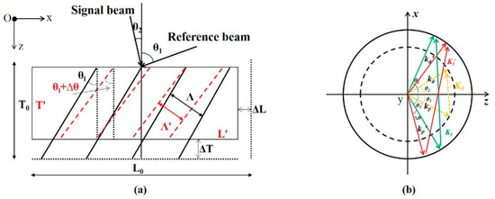
Figure 1.
(a) The schematic diagram for the model of the dimension change in the recording medium; (b) the illustration of the vector diagram in the Ewald sphere.
Assuming the wavelengths of the light for writing and reading are λ and λ’, respectively, λ’ can be expressed as λ’ = λ + Δλ, where Δλ is 0 in the common system without wavelength compensation. Figure 1b illustrates the vector diagram in the Ewald sphere, and the radius of the circle is 2π/λ’. The length of the grating vector K0 is equal to 2π/Λ. Furthermore, the change in the grating period indicates the changes in the length of the grating vector, as illustrated in Figure 1b, in which K0 becomes K1. In addition, if the inclination angle of the grating fringe surface changes either, the direction of the grating vector would be rotated as well, which is illustrated as K1’ in Figure 2b. In the condition that the dimension of the recording medium is changed, the symbol of the grating vector after the change is denoted as K’, then, if the light of reading is incident at the original incident angle θ1 with the original wavelength λ (i.e., λ’ = λ), the three vectors (i.e., the read light vector kp, the grating vector K’ and the reconstructed light vector kd) cannot form a closed triangle, which means the Bragg condition cannot be matched, and the diffraction efficiency would be sharply reduced. As shown in Figure 1b, the incident angle of the readout light or the wavelength of the reading light should be adjusted so as to make the three vectors re-form a closed triangle and match the Bragg condition, then reacquire a high diffraction efficiency. The wavelength adjustment (Δλ ≠ 0) is similar to that in the compensation for the off-axis system, whereas, due to the fact that hologram writing and reading are performed in a single optical path in a collinear system, the incident angle of the reading light cannot be directly adjusted.
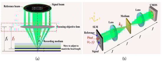
Figure 2.
The illustrations of (a) the principle for the focal length compensation in the collinear holographic storage system, and (b) the simplified optical path of the collinear holographic storage system.
In this paper, the incident angle was adjusted by changing the focal length of the objective lens. Figure 2a illustrates the principle of the focal length compensation; the light beam on the SLM was focused by the objective lens into the recording medium, and the angles of the light beam directed at the material were determined by the focal length of the focusing objective lens (e.g., in Figure 2a, the focal length f1 corresponds to θ1, and f2 corresponds to θ2). Then, based on increasing or decreasing the focal length of the lens, the angles of the reading light could be adjusted, and the inferior reconstructed hologram caused by the material dimension change could be repaired and compensated. To clarify, Figure 2 only illustrates the schematic diagrams; the real holographic storage system is more complex, as fine-tuning the focal length could be realized by shifting the relative positions of the relay lens module in the system, and the achromatic lens would be used in the real system.
As shown in Figure 2b, the light wave emitted from each pixel (xi, yj) on the SLM would be a plane wave incident into the recording medium after propagating through the focusing objective lens. In the writing procedure, the k vector of the plane wave is given by Equation (1) [35], where k0 is equal to 2π/λ, f is the focal length of the lens and n is the refractive index of the recording medium. The grating vector written by the plane waves from two different pixels on the SLM can be calculated by the subtraction of the two k vectors [35].
The grating vector K0 formed by writing is denoted as K0 = [K0x, K0y, K0z], which is the original grating vector. The original length and the thickness of the recording medium are L0 and T0, respectively, and L’ and T’ represent the corresponding dimensions after the volume change of the medium. The rate of dimension change in the lateral plane (σL) is assumed to be isotropic, which is defined by Equation (2), and the vertical dimension change rate (σV) is defined by Equation (3). When the dimension of the recording medium has been changed, the corresponding grating vector K’ is described by Equation (4).
In the reading procedure, the k vector of the reading wave, which corresponds to the pixel (xrk,yrl) in the reading light pattern on the SLM, is given as Equation (5), where k’0 = 2π/λ’ = 2π/(λ + Δλ) and Δf is the amount of change in focal length (the focal length after adjustment is f’, which is equal to f + Δf).
Then, the complex amplitude of the diffracted light wave can be calculated by the Kogelnik theory [34], and under the condition that the dimension of the recording medium has been changed, the reconstructed hologram with the compensation can be obtained by the sum of all the waves emitted from all the pixels in the reading light pattern and diffracted by all the gratings in the medium.
The bit error ratio (BER) defined by Equation (6) was used to evaluate the quality of the reconstructed hologram and was an indicator of the effect of the compensation method.
where Nerror represents the number of the symbol units with errors in the reconstructed signal light pattern, and Ntotal is the total number of symbols in the original signal pattern, and each symbol corresponds to a block of 4 × 4 pixels on the SLM.
2.2. Parameters in the Simulation
Figure 3 is the intensity pattern of the signal light pattern and the reference light pattern, in which the illumination was spatially coherent. The outside pattern was the reference light as shown in Figure 3b, for which the radial line reference pattern was used [35], and the inner pattern was the signal data page, which had 12 symbols in both the length and width directions and contained four sync marks for location [36]. The wavelength of the light for writing was 532 nm, the pixel pitch of the SLM was 13.7 μm and the original focal length for the achromatic objective lens was 5 mm. Furthermore, the diffracted light from each single pixel in the SLM was in the Fraunhofer region directly in front of the lens [35]. The thickness of the medium was 1 mm, the PQ-PMMA photopolymer was used as the recording medium, the refractive index of the medium was 1.5 and the spatial modulation of the refractive index was 1 × 10⁻⁴.
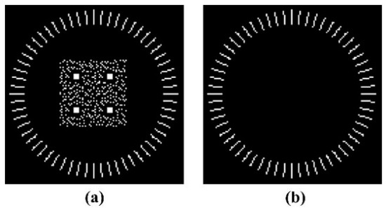
Figure 3.
(a) The reference light pattern and the signal light pattern uploaded on the SLM; (b) the reference light pattern, which is also the reading light pattern.
3. Simulation Results and Discussion
Generally, the dimension change rates of the recording medium in the lateral direction and the vertical direction would be quite different. The lateral dimension change condition (σV ≡ 0) and the vertical dimension change condition (σL ≡ 0) were analyzed respectively, so as to clearly investigate and compare the compensation effects.
Figure 4 shows the BER of the reconstructed signal pattern for different lateral or vertical dimension change rates σ without any compensation. It can be seen that for both kinds of dimension changes, the corresponding BER began to grow when σ reached about 1%, and then the BER increased sharply as σ increased. In addition, it can be also deduced that, compared with the vertical dimension change under the same σ value (σ > 1%), the lateral dimension change could obtain a higher BER, which means the lateral dimension change could influence the quality of the reconstructed hologram more severely than the vertical dimension change.
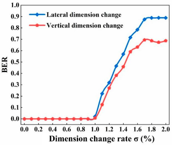
Figure 4.
Without any compensation, the BER of the reconstructed signal pattern for different lateral dimension change rates σL and vertical dimension change rates σV. (σ = σL, σ= σV).
In order to prove the effectiveness of the compensation method, we made an effort to compensate for the conditions when σL and σV were as high as 1.5%, where the BER for the lateral dimension change increased to 0.7153, and the BER for the vertical dimension change was 0.5417.
Firstly, the compensation that only utilized the wavelength adjustment was implemented, and Figure 5 depicts the results for the lateral dimension change condition and the vertical dimension change condition. Although there was a large adjustment range for decreasing or increasing the wavelength (i.e., Δλ∈[−20, 20] nm, where the wavelength interval was 1 nm, and each wavelength comes from a narrow-band laser), the BER did not reach zero for either kind of dimension change condition, and the BER was not significantly reduced. Under the lateral dimension change condition, the minimum BER only decreased to 0.5903, though the wavelength needed to be decreased by 19 nm, which we attempted to no avail. Then, under the vertical dimension change condition, the minimum BER decreased to 0.4583 while the wavelength only increased by 4 nm.
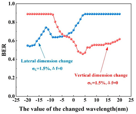
Figure 5.
The BER with different wavelength adjustments of the reading light for the lateral dimension change condition (σL = 1.5%) and the vertical dimension change condition (σV = 1.5%) when the focal length of the objective lens was unchanged.
Secondly, the compensation based on changing the focal length of the objective lens was implemented as a comparison, and the results shown in Figure 6 indicate that the compensation effect was better than that of the former wavelength compensation method, and the BER was reduced to zero both for the lateral dimension change condition and the vertical dimension change condition. As can be seen from Figure 6, the focal length range of zero BER for the vertical dimension change condition (i.e., (65, 25) μm, about 40 μm) was larger than that of the lateral dimension change condition (i.e., (40, 45) μm, about 5 μm), which means it would be easier to adjust to zero BER for the vertical dimension change condition. From the results in Figure 5 and Figure 6, it can be deduced that the compensation for the lateral dimension change condition would be more difficult to achieve than for the vertical dimension change condition if they were to confront the same σ value.
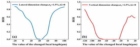
Figure 6.
The BER with different objective focal length adjustments for (a) the lateral dimension change condition (σL = 1.5%) and (b) the vertical dimension change condition (σV = 1.5%) when the wavelength of the reading light was unchanged.
As shown in Figure 6a, the focal length adjustment range for reducing the BER to zero was narrow for the lateral dimension change condition. In order to widen the focal length adjustment range for compensation, the combination compensation method of simultaneously adjusting the focal length and the wavelength was introduced. Considering the lateral dimension change curve in Figure 5, when the wavelength decreased by 9 nm (i.e., −9 nm), though it did not achieve the smallest BER value, it still corresponded to the local minimum value, 0.6389; thus, the focal length adjustment was implemented and analyzed under the condition that the wavelength was decreased by 9 nm, and Figure 7 shows the results of this combination compensation method for the lateral dimension change condition. It can be observed that on the basis of the wavelength adjustment, the corresponding focal length adjustment range for compensation was (30, 80) μm, and the range width was 10 times that shown in Figure 6a. It needs to be clarified that the focal length change with the wavelength change induced by dispersion was not considered in the simulations, as such a focal length change would be too small to be considered if an achromatic lens were to be used, since the wavelength change would only be tens of nanometers.
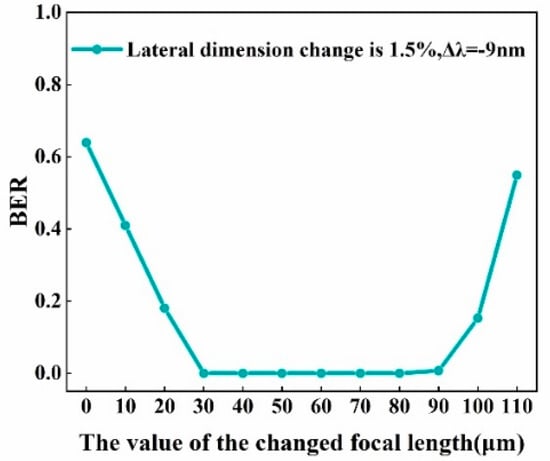
Figure 7.
The BER with different focal length adjustments when the wavelength of the reading light was reduced by 9 nm and σL was 1.5%.
In order to directly observe and analyze the reconstructed signal patterns related to the results in Figure 7, Figure 8(c1–i1) show the reconstructed signal patterns with focal length changes Δf = 0 μm, 10 μm, 30 μm, 50 μm, 60 μm, 80 μm and 110 μm, respectively, while the wavelength of the reading light was reduced by 9 nm. In comparison, Figure 8(a1,b1) show the reconstructed diagrams without any compensation under σL = 0 and 1.5%, respectively. The pictures denoted as Figure 8(a2–c2), etc., immediately to the right of the reconstructed patterns, are the corresponding symbol error diagrams. In these diagrams, each of the tiny bright squares, denoted as ‘An error symbol’ in Figure 8(d2), represents error within the symbol located there, and the bright space is the composition of these error symbols. The compensation results in Figure 8e–h directly show the effectiveness of this combination compensation method.
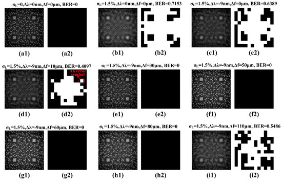
Figure 8.
(a) The reconstructed signal pattern without the dimension change of the recording medium; (b) the reconstructed signal pattern with σL = 1.5% and without any compensation. When σL = 1.5%, for the reconstructed signal patterns with the combination compensation method, the reading light wavelength was decreased by 9 nm and the focal length was changed by (c) 0 μm, (d) 10 μm, (e) 30 μm, (f) 50 μm, (g) 60 μm, (h) 80 μm and (i) 110 μm. The corresponding symbol error diagrams are depicted to the right of the correlated reconstructed signal patterns.
The normalized pixel intensity histogram was used to analyze the reconstructed signal pattern, as shown in Figure 9, where the abscissa represents the normalized intensity of each pixel, and the vertical axis represents the quantity of the pixels with a certain intensity. Figure 9a corresponds to the reconstructed signal pattern in Figure 8(a1), which is the original one without any dimension change of the medium. It can be observed from Figure 9a that the intensities of the ‘bright pixels’ were mainly distributed within the abscissa value within (0.8, 1), while the intensities of the ‘dark pixels’ were mainly distributed within (0, 0.4), and there was no overlapping between the dark and the bright pixels along the abscissa, which means the dark and the bright spots can be clearly distinguished. However, when the dimension change occurred in the material with σL = 1.5%, the intensity distribution of the dark and the bright pixels became consecutive, as shown in Figure 9b. In Figure 9c,d,i, when the wavelength decreased by 9 nm, the focal length was not sufficient to ensure an effective compensation. When the focal length adjustment increased to the range of (30, 80) µm, as shown in Figure 9e–h, the dark and the bright pixels were separated again without overlapping along the abscissa. The results also suggest that the combination compensation method of the focal length and the wavelength adjustments can maintain a BER of 0 in a larger selection range of focal length.
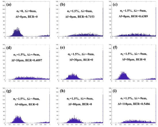
Figure 9.
The normalized pixel distribution histograms of (a) the original reconstructed signal pattern; (b) the reconstructed signal pattern under σL was 1.5% and without any compensation; the reconstructed signal patterns under σL were 1.5% with the combination compensation method, in which the reading light wavelength was decreased by 9 nm and the focal length was changed by (c) 0 μm, (d) 10 μm, (e) 30 μm, (f) 50 μm, (g) 60 μm, (h) 80 μm and (i) 110 μm.
To further demonstrate the feasibility of the combination compensation method for the lateral dimension change condition (σL = 1.5%) and the vertical dimension change condition (σV = 1.5%), we systematically analyzed the compensation effects by varying the wavelength and the focal length of the objective lens in a large scope. The compensation effects are shown in Figure 10; it can be seen that for both of the lateral dimension change and the vertical dimension change, the scopes when adjusting the wavelength and the focal length for realizing zero BER compensation are relatively large. There are plenty of combinations of wavelength and focal length that result in a BER value of zero, for which one-to-one correspondence between the wavelength and the focal length is not required, whereas under the different wavelength values, the range of options for the focal length adjustment would be different. It is suggested that the wavelength compensation be scanned first, as under a wavelength which leads to a smaller BER, the range for a successful focal length compensation would be larger. Compared with the compensation method, which only adjusts the wavelength or the focal length, the combination compensation method can enlarge the compensation scope and thus increase the robustness of the collinear system.
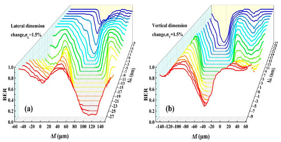
Figure 10.
The compensation effects of the combination compensation method for (a) the lateral dimension change condition (σL = 1.5%) and (b) the vertical dimension change condition (σV = 1.5%).
4. Conclusions
In this paper, we systematically analyzed a combination method of simultaneously adjusting the focal length and the reading light wavelength for compensating large dimensional change within the recording medium in a collinear holographic storage system and compared the compensation effects under lateral dimension change and vertical dimension change conditions. The analysis suggests that though the compensation for the lateral dimension change would be more difficult to achieve than that for the vertical dimension change, this combination compensation method can decrease the BER to 0 with a large adjustment scope both for the lateral and vertical dimension change conditions under a high dimension change rate (σL = 1.5%, σV = 1.5%). The combination compensation method can enlarge the adjustment scope, and the two adjustment parameters (the wavelength of the reading light and the focal length of the lens) do not need to be in one-to-one correspondence to each other. The large compensation scope would facilitate the experiment, and the simulation results can be used to instruct the implementation of collinear holographic storage systems. Based on results achieved for the combination compensation method, the tolerance of the volume change in the recording medium in a collinear holographic storage system could be improved as well.
Author Contributions
Conceptualization, X.T.; methodology, K.W., X.L. and D.L.; validation, X.Q., K.W. and X.L.; data curation, J.H., Q.Z., R.C. and S.W.; writing—original draft preparation, X.Q. and K.W.; writing—review and editing, K.W. and X.Q.; project administration, X.L. and K.W.; funding acquisition, X.T. and K.W. All authors have read and agreed to the published version of the manuscript.
Funding
This research was funded by the National Key Research and Development Program of China (2018YFA0701800), National Natural Science Foundation of China (NSFC) (62005048) and the Major Science & Technology Project of Fujian Province (2020HZ01012).
Conflicts of Interest
The authors declare no conflict of interest.
References
- Dhar, L.; Curtis, K.; FäCke, T. Holographic data storage: Coming of age. Nat. Photonics 2008, 2, 403–405. [Google Scholar] [CrossRef]
- Heanue, J.F.; Bashaw, M.C.; Hesselink, L. Volume holographic storage and retrieval of digital data. Science 1994, 265, 749–752. [Google Scholar] [CrossRef] [PubMed]
- Hao, J.; Lin, X.; Lin, Y.; Song, H.; Chen, R.; Chen, M.; Wang, K.; Tan, X. Lensless phase retrieval based on deep learning used in holographic data storage. Opt. Lett. 2021, 46, 4168–4171. [Google Scholar] [CrossRef]
- Lin, X.; Liu, J.; Hao, J.; Wang, K.; Zhang, Y.; Li, H.; Horimai, H.; Tan, X. Collinear holographic data storage technologies. Opto-Electronic Adv. 2020, 3, 190004. [Google Scholar] [CrossRef]
- Liu, J.; Zhang, L.; Wu, A.; Tanaka, Y.; Shigaki, M.; Shimura, T.; Lin, X.; Tan, X. High noise margin decoding of holographic data page based on compressed sensing. Opt. Express 2020, 28, 7139–7151. [Google Scholar] [CrossRef] [PubMed]
- Lin, X.; Hao, J.; Zheng, M.; Dai, T.; Li, H.; Ren, Y. Optical holographic data storage—The time for new development. Opto-Electron. Eng. 2019, 46, 180642. [Google Scholar]
- Nobukawa, T.; Nomura, T. Linear phase encoding for holographic data storage with a single phase-only spatial light modulator. Appl. Opt. 2016, 55, 2565–2573. [Google Scholar] [CrossRef]
- Nobukawa, T.; Nomura, T. Design of high-resolution and multilevel reference pattern for improvement of both light utilization efficiency and signal-to-noise ratio in collinear holographic data storage. Appl. Opt. 2014, 53, 3773–3781. [Google Scholar] [CrossRef]
- Jia, W.; Chen, Z.; Wen, F.J.; Zhou, C.; Chow, Y.; Chung, P.S. Collinear holographic encoding based on pure phase modulation. Appl. Opt. 2011, 50, H10–H15. [Google Scholar] [CrossRef]
- Minabe, J.; Ogasawara, Y.; Yasuda, S.; Kawano, K.; Hayashi, K.; Yoshizawa, H.; Haga, K.; Furuki, M. Multilayer Holographic Storage Using Collinear Optical Systems. Jpn. J. Appl. Phys. 2008, 47, 5968–5970. [Google Scholar] [CrossRef]
- Horimai, H.; Tan, X.; Li, J. Collinear holography. Appl. Opt. 2005, 44, 2575–2579. [Google Scholar] [CrossRef] [PubMed]
- Li, J.; Cao, L.; Gu, H.; Tan, X.; He, Q. Wavelength and defocus margins of the collinear holographic storage system. SPIE 2010, 7851, 7851115. [Google Scholar]
- Horimai, H.; Tan, X. Holographic Information Storage System: Today and Future. IEEE Trans. Magn. 2007, 43, 943–947. [Google Scholar] [CrossRef]
- Yasuda, S.; Ogasawara, Y.; Minabe, J.; Kawano, K.; Yoshizawa, H. Optical noise reduction by reconstructing positive and negative images from fourier holograms in collinear holographic storage systems. Opt. Lett. 2006, 31, 1639–1641. [Google Scholar] [CrossRef]
- Mohesh, M.; Viswanath, B.; Manojit, P.; Vincent, T.; Izabela, N. Application of phase shifting electronic speckle pattern interferometry in studies of photoinduced dimension change of photopolymer layers. Opt. Express 2017, 25, 9647–9653. [Google Scholar]
- Fernández, R.; Gallego, S.; Navarro-Fuster, V.; Neipp, C.; Francés, J.; Fenoll, S.; Pascual, I.; Beléndez, A. Dimensional changes in slanted diffraction gratings recorded in photopolymers. Opt. Mater. Express 2016, 6, 3455–3468. [Google Scholar] [CrossRef] [Green Version]
- Moothanchery, M.; Naydenova, I.; Toal, V. Studies of dimension change as a result of holographic recording in acrylamide-based photopolymer film. Appl. Phys. A-Mater. 2011, 104, 899–902. [Google Scholar] [CrossRef] [Green Version]
- Moothanchery, M.; Naydenova, I.; Mintova, S.; Toal, V. Nanozeolites doped photopolymer layers with reduced dimension change. Opt. Express 2011, 19, 25786–25791. [Google Scholar] [CrossRef] [Green Version]
- Moothanchery, M.; Bavigadda, V.; Toal, V.; Naydenova, I. Shrinkage during holographic recording in photopolymer films determined by holographic interferometry. Appl. Opt. 2013, 52, 8519–8527. [Google Scholar] [CrossRef]
- Liu, Y.; Fan, F.; Hong, Y.; Zang, J.; Kang, G.; Tan, X. Volume holographic recording in irgacure 784-doped PMMA photopolymer. Opt. Express 2017, 25, 20654–20662. [Google Scholar] [CrossRef]
- Toishi, M.; Tanaka, T.; Watanabe, K. Analysis of temperature change effects on hologram recordingand a compensation method. Opt. Rev. 2008, 15, 11–18. [Google Scholar] [CrossRef]
- Tanaka, T.; Sako, K.; Kasegawa, R.; Toishi, M.; Watanabe, K. Tunable blue laser compensates for thermal expansion of the medium in holographic data storage. Appl. Opt. 2007, 46, 6263–6272. [Google Scholar] [CrossRef] [PubMed]
- Aswathy, G.; Rajesh, C.S.; Kartha, C.S. Multiplexing recording in nickel-ion-doped photopolymer material for holographic data storage applications. Appl. Opt. 2017, 56, 1566–1573. [Google Scholar] [CrossRef]
- Neipp, C.; Taleb, S.I.; Francés, J.; Fernández, R.; Beléndez, A. Analysis of the Imaging Characteristics of Holographic Waveguides Recorded in Photopolymers. Polymers 2020, 12, 1485. [Google Scholar] [CrossRef]
- Fan, F.; Liu, Y.; Hong, Y.; Zang, J.; Wu, A.; Zhao, T.; Kang, G.; Tan, X.; Shimura, T. Improving the polarization-holography performance of PQ/PMMA photopolymer by doping with THMFA. Opt. Express 2018, 26, 17794–17803. [Google Scholar] [CrossRef]
- Dhar, L.; Schnoes, M.G.; Wysock, T.L.; Bair, H.; Schilling, M.; Boyd, C. Temperature-induced changes in photopolymer volume holograms. Appl. Phys. Lett. 1998, 73, 1337–1339. [Google Scholar] [CrossRef]
- Tomiji, T. Recording and reading temperature tolerance in holographic data storage, in relation to the anisotropic thermal expansion of a photopolymer medium. Opt. Express 2009, 17, 14132–14142. [Google Scholar]
- Ishii, N.; Muroi, T.; Kinoshita, N.; Kamijo, K.; Shimidzu, N. Wavefront compensation method using novel index in holographic data storage. J. Eur. Opt. Soc-Rapid 2010, 5, 10036s. [Google Scholar] [CrossRef]
- Toishi, M.; Tanaka, T.; Sugiki, M.; Watanabe, K. Improvement in temperature tolerance of holographic data storage using wavelength tunable laser. Jpn. J. Appl. Phys. 2006, 45, 1297–1304. [Google Scholar] [CrossRef]
- Toishi, M.; Tanaka, T.; Sugiki, M.; Watanabe, K. Temperature tolerance improvement with wavelength tuning laser source in holographic data storage. In Proceedings of the International Symposium on Optical Memory and Optical Data Storage, OSA Technical Digest Series (Optical Society of America), Honolulu, HA, USA, 10–14 July 2005. [Google Scholar]
- Toishi, M.; Tanaka, T.; Fukumoto, A.; Sugiki, M.; Watanabe, K. Evaluation of polycarbonate substrate hologram recording medium regarding implication of birefringence and thermal expansion. Opt. Commun. 2007, 270, 17–24. [Google Scholar] [CrossRef]
- Toishi, M.; Tanaka, T.; Watanabe, K. Experimental analysis in recording transmission and reflection holograms at the same time and location. Appl. Opt. 2006, 45, 6367–6373. [Google Scholar] [CrossRef]
- Ito, T.; Tanaka, K.; Mori, H.; Tanaka, T.; Ishioka, K.; Fukumoto, A.; Okada, K. Improvement in Temperature Tolerance of Collinear Holographic Data Storage. In Proceedings of the 2009 Optical Data Storage Topical Meeting, Lake Buena Vista, FL, USA, 10–13 May 2009; pp. 87–89. [Google Scholar]
- Kogelnik, K. Coupled-wave theory for thick hologram gratings. Bell Syst. Tech. J. 1969, 48, 2909–2947. [Google Scholar] [CrossRef]
- Shimura, T.; Ichimura, S.; Fujimura, R.; Kuroda, K.; Tan, X.; Horimai, H. Analysis of a collinear holographic storage system: Introduction of pixel spread function. Opt. Lett. 2006, 31, 1208–1210. [Google Scholar] [CrossRef]
- King, B.M.; Neifeld, M.A. Sparse modulation coding for increased capacity in volume holographic storage. Appl. Opt. 2000, 41, 1763–1766. [Google Scholar] [CrossRef]
Publisher’s Note: MDPI stays neutral with regard to jurisdictional claims in published maps and institutional affiliations. |
© 2022 by the authors. Licensee MDPI, Basel, Switzerland. This article is an open access article distributed under the terms and conditions of the Creative Commons Attribution (CC BY) license (https://creativecommons.org/licenses/by/4.0/).