Article

Tailoring of Inverse Energy Flow Profiles with Vector Lissajous Beams

by
Svetlana N. Khonina
1,2,
Alexey P. Porfirev
1,
Andrey V. Ustinov
1,
Mikhail S. Kirilenko
2 and
Nikolay L. Kazanskiy
1,2,*
1
IPSI RAS—Branch of the FSRC “Crystallography and Photonics” RAS, Molodogvardeyskaya 151, 443001 Samara, Russia
2
Department of Technical Cybernetics, Samara National Research University, Moskovskoye Shosse 34, 443086 Samara, Russia
*
Author to whom correspondence should be addressed.
Photonics 2022, 9(2), 121; https://doi.org/10.3390/photonics9020121
Submission received: 26 January 2022 / Revised: 17 February 2022 / Accepted: 18 February 2022 / Published: 20 February 2022
(This article belongs to the Special Issue Polarized Light and Optical Systems)

Abstract

:
In recent years, structured laser beams for shaping inverse energy flow regions: regions with a direction of energy flow opposite to the propagation direction of a laser beam, have been actively studied. Unfortunately, many structured laser beams generate inverse energy flow regions with dimensions of the order of the wavelength. Moreover, there are significant limitations to the location of these regions. Here, we investigate the possibility of controlling inverse energy flow distributions by using the generalization of well-known cylindrical vector beams with special polarization symmetry—vector Lissajous beams (VLBs)—defined by two polarization orders (p, q). We derive the conditions for the indices (p, q) in order, not only to shape separate isolated regions with a reverse energy flow, but also regions that are infinitely extended along a certain direction in the focal plane. In addition, we show that the maximum intensity curves of the studied VLBs are useful for predicting the properties of focused beams.

1. Introduction

It is well-known that structured laser beams with the desired amplitude, phase, and/or polarization distribution are beginning to find more and more applications in various fields of science and technology [1]; many excellent reviews are devoted to the application of such beams in optical communications [2], laser manipulation [3,4], and laser material processing [5], etc. [6]. In recent years, structured laser beams to shape inverse energy flow regions have been actively studied. Inverse energy flow means that the direction of energy flow is opposite to the propagation direction of the beam and is associated with a local change in the sign of the components of the Poynting vector under free propagation [7]. Interest in the investigation of such laser beams is explained by the hope of using such laser beams to pull laser beams that are capable of attracting optically trapped nano- and micro-objects towards a radiation source [8]. If an inverse energy flow is formed on the optical axis, then its presence moves dielectric nanoparticles with absorption in the direction opposite to the propagation of the laser beam, with a greater force than similar particles without absorption. In the absence of an inverse flow, both particles (with and without absorption) move equally [9]. However, just the presence of areas with an inverse energy flow does not guarantee the existence of the attracting optical forces—the gradient-phase force often blocks the effect of the negative Poynting vector component, giving a negative optical force [10,11].
Many different approaches have been used to demonstrate the possibility of shaping inverse energy flow regions—the use of interference patterns generated by four plane waves with linear polarization [12,13], circularly polarized optical vortex (OV) beams [14,15], cylindrical vector beams (CVBs) [16,17,18,19], and OVs with polarization singularities [20]. In all these cases, the dimensions of the region of the formation of the inverse energy flow are small (approximately of the order of the wavelength) and the location of this region is limited by the optical axis. Some techniques were proposed to overcome these limitations—the use of annular apertures for the elongation of the area of energy backflow [21,22] and the use of special generalized spiral phase plates to shift the center of the Poynting vector distribution and the maximum negative value of the inverse energy flow from the optical axis [23].
Here, we investigate the possibility of tailoring the inverse energy flow distributions using the generalization of CVBs—vector Lissajous beams (VLBs)—introduced in 2020 [24]. These beams have more degrees of freedom than conventional CVBs—the structure of these beams is defined by two polarization orders ( p , q ) which can be both integer and fractional. Due to this, VLBs allow one to manage the characteristics of the electromagnetic field, such as the imaginary part of the longitudinal component of the field, the local spin angular momentum (SAM) density, and the complex Poynting vector density [25]. Hao Wu, with co-authors, reported selective trapping of chiral nanoparticles via VLBs due to formed intensity spots with opposite chirality [26]. In addition, the amplitude distributions of VLBs are not limited only to symmetric profiles and are similar to the well-known Lissajous figures, which is why these beams were given this title. All these features of VLBs allow the formation of inverse energy flow regions with different profiles that differ from those previously demonstrated in known works. Thus, VLBs is a convenient tool for more accurate control of the local characteristics of the energy flow and allow one to control light on a nano- and microscale to form a given distribution of forces acting on optically trapped particles.
Previously, the types of VLBs that can be considered as the generalization of radial polarization, namely ( cos ( p φ ) , sin ( q φ ) ), have been considered in detail. In this paper, we study a wider set of polarization states related to VLBs: x- and y-components of these states can have the same trigonometric dependencies, in particular, ( cos ( p φ ) , cos ( q φ ) ) and ( sin ( p φ ) , sin ( q φ ) ). Note that such types of polarizations, even at p = q , do not reduce to known CVBs. This provides new properties of the presented fields. In addition, the possibility of forming a reverse energy flow for focused VLBs has not yet been considered; therefore, such studies are of interest from both fundamental and practical points of view.

2. Theoretical Foundation

The electromagnetic field distribution in a focal domain can be derived by the vectorial diffraction theory [27,28,29,30,31,32,33,34,35,36]. The vector nature of radiation should be taken into account when acting on a substance [3,4,5,6,7,8,9,10,11,37,38], when it propagates in anisotropic or inhomogeneous medium [39,40,41,42], and also at tight focusing [27,28,29,30,31,32,33,34,35,36]. In the latter case, the calculation of the focused field is often performed using the Debye approximation [27,28,29,33,34,35,36]. For tight focusing using the Debye approximation, the electric and magnetic field vectors are determined as follows:
[ E ( ρ , υ , z ) H ( ρ , υ , z ) ] = i f λ 0 α 0 2 π F ( θ , φ ) T ( θ ) [ P E ( θ , φ ) P H ( θ , φ ) ] × exp [ i k ( ρ sin θ cos ( φ υ ) + z cos θ ) ] sin θ d θ d φ ,
where (ρ, υ, z) are the cylindrical coordinates in the focal region, (θ, φ) are the spherical angular coordinates of the focusing system’s output pupil, α is the maximum value of the azimuthal angle θ related to the system’s numerical aperture NA = sinα, k = 2 π / λ is the wavenumber, λ is the radiation wavelength, f is a focal length of an optical system, T ( θ ) is the apodization function; F ( θ , φ ) is a complex amplitude of the field at the exit pupil.
The Debye approximation neglects contributions from diffraction at the edge of the aperture, therefore, the correctness of the results is ensured at a high value of the Fresnel number (i.e., when f >> λ, fsinα >> λ), as well as near the focal plane [43,44,45]. Taking into account these conditions, expression (1) is a convenient tool for calculating the 3D distribution of the vector field in the focal region [46,47,48].
Note, in most articles only the electric component of the field is considered. However, to calculate characteristics such as the Poynting vector, expressions for the magnetic component of the field are also required, which can be calculated using Maxwell’s equations. In Equation (1), the polarization transformation vectors for the electric and magnetic field are the following [18,23,25]:
P E ( θ , φ ) = [ A ( θ , φ ) C ( θ , φ ) C ( θ , φ ) B ( θ , φ ) D ( θ , φ ) E ( θ , φ ) ] ( c x ( θ , φ ) c y ( θ , φ ) ) , P H ( θ , φ ) = [ C ( θ , φ ) A ( θ , φ ) B ( θ , φ ) C ( θ , φ ) E ( θ , φ ) D ( θ , φ ) ] ( c x ( θ , φ ) c y ( θ , φ ) ) ,
where
A ( θ , φ ) = 1 + cos 2 φ ( cos θ 1 ) , B ( θ , φ ) = 1 + sin 2 φ ( cos θ 1 ) , C ( θ , φ ) = sin φ cos φ ( cos θ 1 ) , D ( θ , φ ) = cos φ sin θ , E ( θ , φ ) = sin φ sin θ .
In Equation (2), c ( θ , φ ) = ( c x ( θ , φ ) c y ( θ , φ ) ) is a vector of polarization coefficients of the input field. In [24], the following generalization of cylindrical polarization was considered by introducing two different orders ( p , q ) for the x- and y-components, respectively:
c ( φ ) = ( cos ( p φ + φ x ) sin ( q φ + φ y ) )
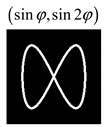
The polarization state defined by Equation (4) was called the Lissajous polarization [
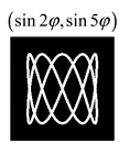
24], since Equation (4) corresponds to the parametric equation of Lissajous figures. Such a figure can be seen in the input field intensity pattern if we draw a curve enveloping the brightest intensity regions.
For the Lissajous polarization defined by Equation (4), one can write the explicit form of the polarization vectors using Equation (2):
P E ( θ , φ ) = ( [ cos ( p φ + φ x ) cos φ + sin ( q φ + φ y ) sin φ ] cos φ cos θ [ sin ( q φ + φ y ) cos φ cos ( p φ + φ x ) sin φ ] sin φ [ cos ( p φ + φ x ) cos φ + sin ( q φ + φ y ) sin φ ] cos φ cos θ + + [ sin ( q φ + φ y ) cos φ cos ( p φ + φ x ) sin φ ] cos φ sin θ [ cos ( p φ + φ x ) cos φ + sin ( q φ + φ y ) sin φ ] )
for P H ( θ , φ ) , the corresponding expression will be similar to Equation (5).
If the input field is factorized as follows:
F ( θ , φ ) = R ( θ ) Φ ( φ )
then, taking into account the possibility of expanding the function Φ ( φ ) in terms of angular harmonics exp ( i n φ ) , the integrals over the angle φ in Equation (1) are calculated analytically [34]. In this case, Equation (1) is reduced to one-dimensional integrals:
[ E ( ρ , υ , z ) H ( ρ , υ , z ) ] = i 2 π f λ 0 α R ( θ ) T ( θ ) [ Q E ( ρ , υ , θ ) Q H ( ρ , υ , θ ) ] exp ( i 2 π λ z cos θ ) sin θ d θ ,
where vectors Q E , H ( ρ , υ , θ ) are superpositions of Bessel functions Jn(sinθ) and angular harmonics.
In particular,
Q E ( ρ , υ , θ ) = 1 4 ( 2 i p ( 1 + cos θ ) J p ( k ρ sin θ ) cos ( p υ + φ x ) + ( 1 cos θ ) [ i p B c 2 p + + i q B c 2 q ] 2 i q ( 1 + cos θ ) J q ( k ρ sin θ ) sin ( q υ + φ y ) ( 1 cos θ ) [ i q B s 2 q + + i p B s 2 p ] 2 sin θ [ i p + 1 B c 1 p + i q + 1 B c 1 q + ] ) ,
where
B c 1 n ± = J n 1 ( k ρ sin θ ) cos [ ( n 1 ) υ + φ n ] ± J n + 1 ( k ρ sin θ ) cos [ ( n + 1 ) υ + φ n ] , B c 2 n ± = J n 2 ( k ρ sin θ ) cos [ ( n 2 ) υ + φ n ] ± J n + 2 ( k ρ sin θ ) cos [ ( n + 2 ) υ + φ n ] , B s 2 n ± = J n 2 ( k ρ sin θ ) sin [ ( n 2 ) υ + φ n ] ± ± J n + 2 ( k ρ sin θ ) sin [ ( n + 2 ) υ + φ n ] , φ n = { φ x , n = p , φ y , n = q .
In Refs. [24,25], special cases of polarization states defined by Equation (4) at φ x = φ y = 0 were studied. In this paper, we consider a wider set of polarization states defined by Equation (4), when the values of φ x , φ y = { 0 , π / 2 } , i.e., the x- and y-components can have the same trigonometric relationships, but with different frequencies ( p , q ) .
To analyze the characteristics of the energy flow associated with the polarization state defined by Equation (4), it is necessary to calculate the Poynting vector:
S E * × H
where E and H are the vectors of the electric and magnetic fields, respectively, calculated using Equation (1) at a fixed value of the parameter z, for example, at z = 0 (i.e., in the focal plane).

3. Theoretical Analysis

Although several recent works consider all components of the Poynting vector, including the imaginary parts of the transverse components [25,49,50,51], in this study we will focus on the analysis of only the longitudinal component (in a complex form):
S z E x * H y E y * H x = Re ( S z ) + i Im ( S z )
In this case, in the real part of Equation (10), we will be especially interested in the areas of negative values, i.e., reverse flow of energy. Since the longitudinal component of the Poynting vector is determined only by the transverse components of the field defined by Equation (1), we will consider only them in the further analysis.
Note, even if the input field does not depend on the azimuth angle, i.e., Φ ( φ ) = const , the components of the polarization vector are composed by angular harmonics exp ( i n φ ) . In this case, it is convenient to represent fields defined by Equation (1) in the focal plane ( z = 0 ) as a superposition of the following integrals:
I n ± ( ρ ) = 0 α R ( θ ) T ( θ ) [ ( 1 ± cos θ ) J n ( k ρ sin θ ) ] sin θ d θ
In Refs. [18,21,23], the field R ( θ ) was considered in combination with a superimposed narrow annular aperture [52]:
D 0 ( θ ) = { 1 , | θ θ 0 | Δ / 2 , 0 , else ,
where Δ is the aperture ring width and θ 0 is the position of the ring center.
In this case, an increased reverse energy flow area is provided [21]. In addition, integrals defined by Equation (11) take the explicit form:
I n ± ( ρ ) Δ J n ( k ρ sin θ 0 ) T ( θ 0 ) ( 1 ± cos θ 0 ) sin θ 0
Let us consider several particular cases of polarization in the form defined by Equation (4).

3.1. Cos-Sin Vector Lissajous Beams (cs-VLBs)

When φ x = φ y = 0 instead of Equation (4) the result is:
c ( φ ) = ( cos ( p φ ) sin ( q φ ) )
Then, the transverse components of the field defined by Equation (1) take the following form (taking into account Equation (11)):
E c s ( ρ , υ , 0 ) = k f 4 × × ( i p + 1 [ 2 I p + cos p υ + I p 2 cos ( p 2 ) υ + I p + 2 cos ( p + 2 ) υ ] + i q + 1 [ I q 2 cos ( q 2 ) υ I q + 2 cos ( q + 2 ) υ ] i q + 1 [ 2 I q + sin q υ I q 2 sin ( q 2 ) υ I q + 2 sin ( q + 2 ) υ ] i p + 1 [ I p 2 sin ( p 2 ) υ I p + 2 sin ( p + 2 ) υ ] ) , H c s ( ρ , υ , 0 ) = k f 4 × × ( i q + 1 [ 2 I q + sin q υ + I q 2 sin ( q 2 ) υ + I q + 2 sin ( q + 2 ) υ ] i p + 1 [ I p 2 sin ( p 2 ) υ I p + 2 sin ( p + 2 ) υ ] i p + 1 [ 2 I p + cos p υ I p 2 cos ( p 2 ) υ I p + 2 cos ( p + 2 ) υ ] i q + 1 [ I q 2 cos ( q 2 ) υ I q + 2 cos ( q + 2 ) υ ] ) .
Based on Equation (15), it can be shown that the longitudinal component consists of two terms:
S z c s = S z 1 c s + S z 2 c s
where S z 1 c s is always real, and the form of S z 2 c s depends on the parity of p and q values.
Explicitly, the first term is
S z 1 c s = 1 4 [ ( I p + cos p υ ) 2 + ( I q + sin q υ ) 2 ] 1 16 [ ( I p 2 ) 2 + ( I p + 2 ) 2 + ( I q 2 ) 2 + ( I q + 2 ) 2 ] 1 8 [ I p 2 I p + 2 cos 2 p υ I q 2 I q + 2 cos 2 q υ ] .
To determine the regions of the reverse energy flow, it is necessary to determine the regions of negative values of Equation (17). Obviously, under the condition cos ( p υ ) = 0 and sin ( q υ ) = 0 , the expression in the first square bracket vanishes. In the third square bracket, this condition is cos ( 2 p υ ) = 1 and cos ( 2 q υ ) = 1 . Taking into account the fact that the expression in the second square bracket does not depend on the angle, instead of Equation (17) we obtain the following expression for the considered angles:
υ i n v c s { cos p υ = 0 & sin q υ = 0 } , S z 1 c s ( υ i n v c s ) = [ ( I p 2 I p + 2 ) 2 + ( I q 2 I q + 2 ) 2 ] < 0 .
Thus, in the areas corresponding to directions with angles υ i n v c s , the first part of Equation (16) has negative values.
An analysis of the directions for different indices ( p , q ) is given in Section 4. Note that these directions do not depend on the size of the entrance pupil and, therefore, do not change when a narrow annular aperture is applied.
Let us now consider the second part, which essentially depends on the parity of the indices ( p , q ) . It can be shown that
S z 2 c s = { S z 2 , e c s , ( p q ) = 4 s , i S z 2 , o c s , ( p q ) = 4 s + 1 , S z 2 , e c s , ( p q ) = 4 s + 2 , i S z 2 , o c s , ( p q ) = 4 s + 3 ,
where
S z 2 , e c s = 1 8 cos ( ( p + q ) υ ) [ I p 2 I q + 2 I p + 2 I q 2 ] + 1 8 cos ( ( p q ) υ ) [ I p + 2 I q + 2 I p 2 I q 2 ] , S z 2 , o c s = 1 4 I p + cos ( p υ ) [ I q 2 cos ( q 2 ) υ I q + 2 cos ( q + 2 ) υ ] + 1 4 I q + sin ( q υ ) [ I p 2 sin ( p 2 ) υ I p + 2 sin ( p + 2 ) υ ] .
As follows from Equation (19), the longitudinal component of the Poynting vector has an imaginary part Im ( S z c s ) 0 only for an odd index difference ( p q ) .
Note that on the directions determined by Equation (18), Equation (19) is equal to zero, i.e., S z 2 c s ( υ i n v c s ) = 0 , so the negative values of the real part of the longitudinal component of the Poynting vector are determined only by Equation (18): Re [ S z c s ( υ i n v c s ) ] < 0 .
We note that there is a significant difference between Equation (18) and a similar equation in Ref. [21], where a beam with a linear x-polarization and a trigonometric amplitude was considered. The expression obtained in Ref. [21] included directions with a zero value of the longitudinal component of the Poynting vector, which did not ensure the connectivity of regions with a reverse energy flow. Under the condition defined in Equation (18), there is a sum of two squares which cannot be equal to zero at the same time for ( p q ) , therefore, the negative value of the longitudinal component of the Poynting vector and the connectivity of the region of the reverse energy flow along a certain direction are guaranteed.

3.2. Cos-Cos Vector Lissajous Beams (cc-VLBs)

When φ x = 0 , φ y = π / 2 instead of Equation (4), we obtain:
c ( φ ) = ( cos ( p φ ) cos ( q φ ) )
Then, the transverse components of the field defined by Equation (1) take the following form:
E c c ( ρ , υ , 0 ) = k f 4 × × ( i p + 1 [ 2 I p + cos p υ + I p 2 cos ( p 2 ) υ + I p + 2 cos ( p + 2 ) υ ] i q + 1 [ I q 2 sin ( q 2 ) υ I q + 2 sin ( q + 2 ) υ ] i q + 1 [ 2 I q + cos q υ I q 2 cos ( q 2 ) υ I q + 2 cos ( q + 2 ) υ ] i p + 1 [ I p 2 sin ( p 2 ) υ I p + 2 sin ( p + 2 ) υ ] ) , H c c ( ρ , υ , 0 ) = k f 4 × × ( i q + 1 [ 2 I q + cos q υ + I q 2 cos ( q 2 ) υ + I q + 2 cos ( q + 2 ) υ ] i p + 1 [ I p 2 sin ( p 2 ) υ I p + 2 sin ( p + 2 ) υ ] i p + 1 [ 2 I p + cos p υ I p 2 cos ( p 2 ) υ I p + 2 cos ( p + 2 ) υ ] + i q + 1 [ I q 2 sin ( q 2 ) υ I q + 2 sin ( q + 2 ) υ ] ) .
As in the previous case, it can be shown that
S z 1 c c = 1 4 [ ( I p + cos p υ ) 2 + ( I q + cos q υ ) 2 ] 1 16 [ ( I p 2 ) 2 + ( I p + 2 ) 2 + ( I q 2 ) 2 + ( I q + 2 ) 2 ] 1 8 [ I p 2 I p + 2 cos 2 p υ + I q 2 I q + 2 cos 2 q υ ] .
Equation (22) takes negative values under the following conditions
υ i n v c c { cos p υ = 0 & cos q υ = 0 } , S z 1 c c ( υ i n v c c ) = [ ( I p 2 I p + 2 ) 2 + ( I q 2 I q + 2 ) 2 ] < 0 .
An analysis of the directions υ i n v c c for different indices ( p , q ) is given in Section 4.
It can also be shown that
S z 2 c c = { S z 2 , e c c , ( p q ) = 4 s , i S z 2 , o c c , ( p q ) = 4 s + 1 , S z 2 , e c c , ( p q ) = 4 s + 2 , i S z 2 , o c c , ( p q ) = 4 s + 3 ,
where
S z 2 , e c c = 1 8 sin ( ( p + q ) υ ) [ I p 2 I q + 2 I p + 2 I q 2 ] + 1 8 sin ( ( p q ) υ ) [ I p + 2 I q + 2 I p 2 I q 2 ] , S z 2 , o c c = 1 4 I p + cos ( p υ ) [ I q 2 sin ( q 2 ) υ I q + 2 sin ( q + 2 ) υ ] 1 4 I q + cos ( q υ ) [ I p 2 sin ( p 2 ) υ I p + 2 sin ( p + 2 ) υ ] .
Similar to the previous case, the longitudinal component of the Poynting vector has an imaginary part Im ( S z c s ) 0 only for an odd index difference ( p q ) .
Additionally, under conditions defined by Equation (23), Equation (24) is equal to zero, i.e., S z 2 c c ( υ i n v c c ) = 0 , so the negative values of the real part of the longitudinal component of the Poynting vector are determined only by Equation (23): Re [ S z c c ( υ i n v c c ) ] < 0 .

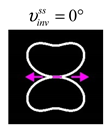
3.3. Sin-Sin Vector Lissajous Beams (ss-VLBs)

When φ x = π / 2 , φ y = 0 instead of Equation (4) we obtain
c ( φ ) = ( sin ( p φ ) sin ( q φ ) )
Then, the transverse components of the field defined by Equation (1) take the following form:
E s s ( ρ , υ , 0 ) = k f 4 × × ( i p + 1 [ 2 I p + sin p υ + I p 2 sin ( p 2 ) υ + I p + 2 sin ( p + 2 ) υ ] + i q + 1 [ I q 2 cos ( q 2 ) υ I q + 2 cos ( q + 2 ) υ ] i q + 1 [ 2 I q + sin q υ I q 2 sin ( q 2 ) υ I q + 2 sin ( q + 2 ) υ ] + i p + 1 [ I p 2 cos ( p 2 ) υ I p + 2 cos ( p + 2 ) υ ] ) , H s s ( ρ , υ , 0 ) = k f 4 × × ( i q + 1 [ 2 I q + sin q υ + I q 2 sin ( q 2 ) υ + I q + 2 sin ( q + 2 ) υ ] + i p + 1 [ I p 2 cos ( p 2 ) υ I p + 2 cos ( p + 2 ) υ ] i p + 1 [ 2 I p + sin p υ I p 2 sin ( p 2 ) υ I p + 2 sin ( p + 2 ) υ ] i q + 1 [ I q 2 cos ( q 2 ) υ I q + 2 cos ( q + 2 ) υ ] ) .
In this case
S z 1 s s = 1 4 [ ( I p + sin p υ ) 2 + ( I q + sin q υ ) 2 ] 1 16 [ ( I p 2 ) 2 + ( I p + 2 ) 2 + ( I q 2 ) 2 + ( I q + 2 ) 2 ] + 1 8 [ I p 2 I p + 2 cos 2 p υ + I q 2 I q + 2 cos 2 q υ ] .
Equation (27) takes negative values under the following conditions:
υ i n v s s { sin p υ = 0 & sin q υ = 0 } , S z 1 s s ( υ i n v s s ) = [ ( I p 2 I p + 2 ) 2 + ( I q 2 I q + 2 ) 2 ] < 0 .
An analysis of directions υ i n v s s for different indices ( p , q ) is given in Section 4.
It can also be shown that
S z 2 s s = { S z 2 , e s s , ( p q ) = 4 s , i S z 2 , o s s , ( p q ) = 4 s + 1 , S z 2 , e s s , ( p q ) = 4 s + 2 , i S z 2 , o s s , ( p q ) = 4 s + 3 ,
where
S z 2 , e s s = 1 8 sin ( ( p + q ) υ ) [ I p 2 I q + 2 I p + 2 I q 2 ] + 1 8 sin ( ( p q ) υ ) [ I p + 2 I q + 2 I p 2 I q 2 ] , S z 2 , o s s = 1 4 I p + sin ( p υ ) [ I q 2 cos ( q 2 ) υ I q + 2 cos ( q + 2 ) υ ] + 1 4 I q + sin ( q υ ) [ I p 2 cos ( p 2 ) υ I p + 2 cos ( p + 2 ) υ ] .
Thus, the results are similar to the previous cases, i.e., Im ( S z s s ) 0 only for an odd index difference ( p q ) . Additionally, under conditions defined by Equation (28), S z 2 s s ( υ i n v s s ) = 0 , therefore Re [ S z s s ( υ i n v s s ) ] < 0 .
It can be seen that although the full expressions for S z at the three considered types of VLBs differ, the conditions defined by Equations (18), (23) and (28) for the values Re ( S z ) in the negative directions are similar. The differences are in the direction angles at which negative values of the real part of the longitudinal component of the Poynting vector are provided, i.e., reverse flow of energy is provided. Therefore, for the same pair of indices ( p , q ) , the number of negative directions is different for the considered types of beams. The differences between the three types of VLBs are discussed in more detail in Section 4.
Note that even if the conditions defined by Equations (18), (23) and (28) are not satisfied, negative values of the longitudinal component are still possible on circles of certain radii, as was considered in Refs. [17,18] for fields with cylindrical polarization. Due to continuity, negative values will not only be on the circles, but also in their neighborhood. Therefore, the overall negative region will have a mesh-cell shape, which was also observed at q = 0 in Ref. [21].

4. Modeling Results

In this section, the following parameters have been used in modeling for narrow annular aperture, defined by Equation (12): θ 0 = 80 ° , Δ = 3.3 ° . Obviously, when the ring width Δ increase, the total energy in the focal area will increase, but the focusing will become less sharp, and the negative energy flow will decrease [21].
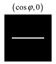
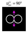
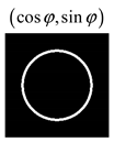
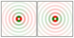
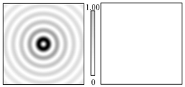
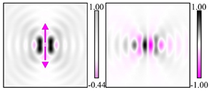
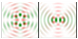
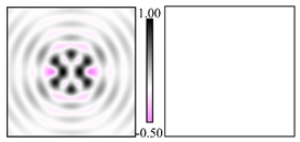
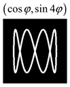
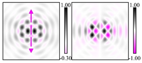
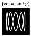
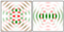
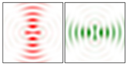
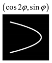
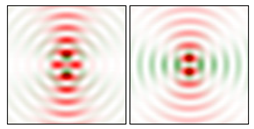
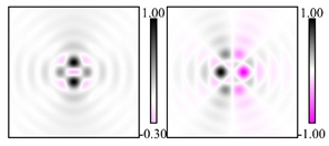
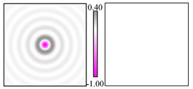
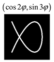
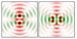
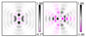
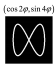
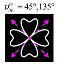
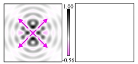
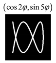
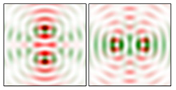
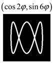
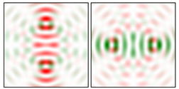
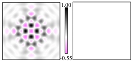
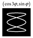
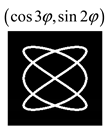
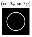
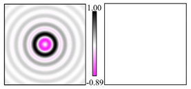
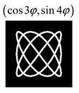
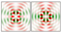
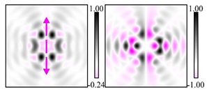
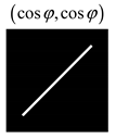
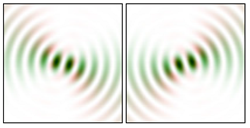
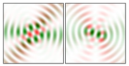
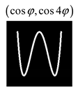
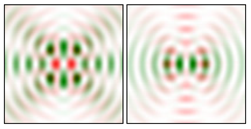
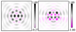
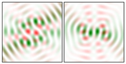
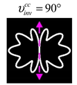
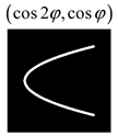
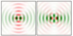
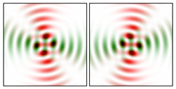
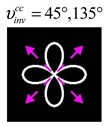
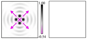
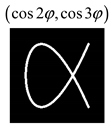
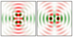
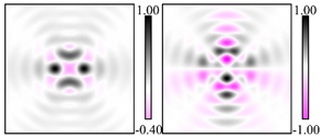
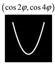
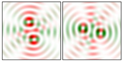
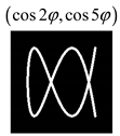
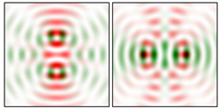
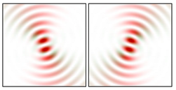
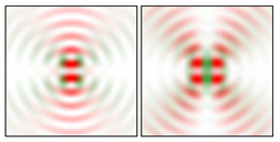
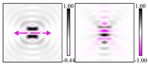
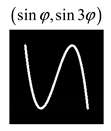
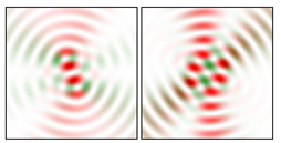
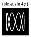
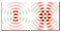
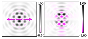
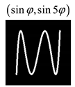
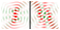
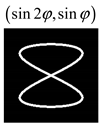
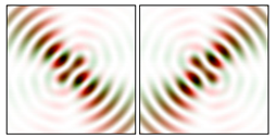
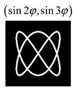
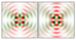
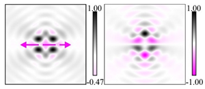
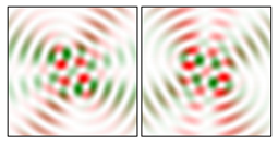
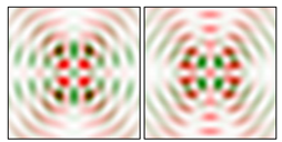
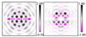
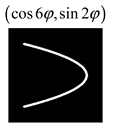
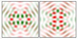
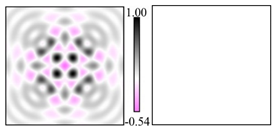
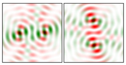
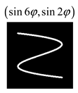
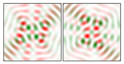
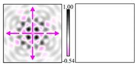
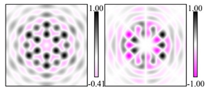
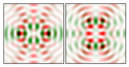
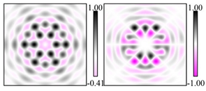
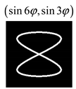
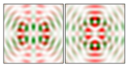
Modeling results contain (see Tables below) the transverse components of electric and magnetic field distributions in the focal plane and distributions of the longitudinal component of the Poynting vector. Moreover, we show the corresponding Lissajous curves (in the first column of Tables):
{ x = cos ( p φ ) , y = sin ( q φ ) ,
and intensity curves [
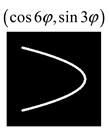
24] (in the third column of tables):
{ x = [ cos 2 ( p φ ) + sin 2 ( q φ ) ] 1 / 2 cos φ , y = [ cos 2 ( p φ ) + sin 2 ( q φ ) ] 1 / 2 sin φ .
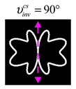
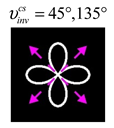
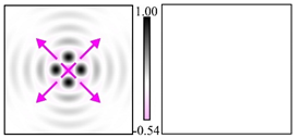
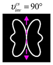
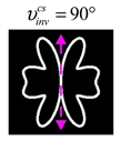
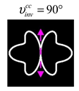
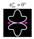
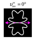
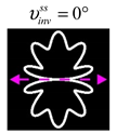
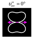
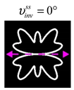
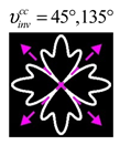
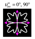
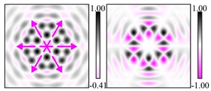
The curve defined by Equation (31) corresponds to the contour of the total intensity distribution in the focal plane. Since the focal intensity is related to the real part of the longitudinal component of the Poynting vector in Equation (10), the intensity curve also corresponds to the structure of Re ( S z ) . By the term “structure” we mean the following: the convex parts of the curve defined by Equation (31) correspond to the locations of maximum positive energy flow, and the concave parts indicate the presence of negative energy flow locations. Infinitely extended regions with Re ( S z ) < 0 are special cases of our investigation. These are directions satisfying the conditions of Equations (18), (23) and (28). We indicate the infinite (unobstructed) directions (regions) with a negative energy flow by magenta arrows, both for Re ( S z ) distributions and for intensity curves.

4.1. Cos-Sin Vector Lissajous Beams (cs-VLBs)

It was shown in Refs. [17,18] that the second-order radial polarization ( p , q ) = ( 2 , 2 ) is optimal from the point of view of maximizing the value of the reverse energy flow on the optical axis. However, the integral characteristic over a region of negative values has been shown theoretically and numerically [18] to increase with the increasing order of radial or azimuthal polarization ( p = q ) . In this case, the real part of the longitudinal component of the Poynting vector has the following form [18]:
Re [ S z c s ( ρ ) | ( p , p ) ] = ( Δ π T ( θ 0 ) sin θ 0 ) 2 × × [ ( 1 + cos θ 0 ) 2 J p 2 ( k ρ sin θ 0 ) ( 1 cos θ 0 ) 2 J p 2 2 ( k ρ sin θ 0 ) ] .
In this case, the areas with negative values of Equation (32) correspond to a set of concentric rings.
In addition, in Ref. [21], a linearly polarized field was considered, which can be considered a special case of cs-VLBs for ( p , q ) = ( p , 0 ) :
Re [ S z c s ( ρ , υ ) | ( p , 0 ) ] = ( 0.5 Δ π T ( θ 0 ) sin θ 0 ) 2 × × { 2 cos 2 ( p υ ) [ ( 1 + cos θ 0 ) 2 J p 2 ( k ρ sin θ 0 ) ( 1 cos θ 0 ) 2 J p 2 ( k ρ sin θ 0 ) J p + 2 ( k ρ sin θ 0 ) ] ( 1 cos θ 0 ) 2 [ J p 2 ( k ρ sin θ 0 ) J p + 2 ( k ρ sin θ 0 ) ] 2 } .
For Equation (33), the achievable value of the reverse flow is less than in the case of radial polarization, however, the region of negative values is not limited (in the annular region) since there are directions with negative values of the energy flow.
In Ref. [23], the results for fields that can be considered cs-VLBs and ss-VLBs for ( p , q ) = ( p , 0 ) were also presented. In addition, the numerical calculation was also made for non-integer p .
The cases considered in this article are more general and may have more unlimited directions of the reverse energy flow.
Table 1, Table 2 and Table 3 show the calculation results for various indices ( p , q ) . We indicate by magenta arrows the infinite (unobstructed) directions (regions) with a negative energy flow both for Re ( S z ) distributions and for intensity curves. As seen, the infinite directions present only when the intensity curve passes through the origin (this also follows from Equation (18)), and the number of such directions is equal to the multiplicity of the zero point of the intensity curve.
One can also notice that there are no negative values Sz in local maxima | E | 2 or | H | 2 . This follows from Equation (9) (if E is close to the maximum, then H × E close to zero, and vice versa).
For the case ( p , q ) = ( 2 , q ) (Table 2), one more feature can be noted: if the Lissajous curve is closed, then Im ( S z c s ) = 0 . For the cases ( p , q ) = ( 1 , q ) (Table 1) and ( p , q ) = ( 3 , q ) (Table 3) there is no such regularity, since all Lissajous curves are closed in these cases.
It can be seen that some distributions are similar up to rotation. This is expected since the polarization functions are trigonometric, but the symmetry properties are quite diverse and difficult to predict from the curve patterns. For example, for ( cos φ , sin 3 φ ) (Table 1) and ( cos 3 φ , sin φ ) (Table 3) Lissajous curves and intensity curves are the same for rotation, but the field distributions and S z are qualitatively different. At the same time, for ( cos 2 φ , sin 3 φ ) (Table 2) and for ( cos 3 φ , sin 2 φ ) (Table 3), the corresponding curves have no similarity at all. This is probably due to the evenness of the indices ( p , q ) .
Let us also note the case ( cos 3 φ , sin 5 φ ) (Table 3). It appears visually from the Re ( S z ) distribution that the diagonal directions are the infinite regions with a negative energy flow. However, in the central part there is a slight interruption of the line with negative Re ( S z ) . For ( cos 3 φ , sin 5 φ ) , the condition of Equation (18) is not met, and the intensity curve do not pass through the origin. So, this is a good example demonstrating the effective visibility of the intensity curve to determine the presence of the infinite regions with a negative energy flow.

4.2. Cos-Cos Vector Lissajous Beams (cc-VLBs)

It can be seen that the structure of the cs-VLBs and cc-VLBs fields for the same indices ( p , q ) is noticeably different. This provides a variety of generated distributions, even for small indices. In some cases, for example, for ( cos φ , cos 2 φ ) (Table 4) and for ( cos 2 φ , cos φ ) (Table 5), the differences are reduced to the rotation of the Lissajous curve and the permutation of the distributions for E and H, which is expected when permuting the polarization functions of the same name.
Note that in the field distributions in the first row of Table 4, the direction along which the maxima are placed has an angle lower than 45 degrees horizontally, although the initial polarization is diagonal. This is a sharp focusing effect that should disappear in a paraxial situation.
In Table 4 and Table 5, all Lissajous curves are open.

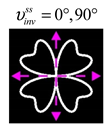
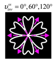
4.3. Sin-Sin Vector Lissajous Beams (ss-VLBs)

For this type of VLBs, some of the distributions are similar to the previous cases and some of the distributions are different. A feature of this type is the presence of infinite directions with a reverse energy flow for arbitrary indices ( p , q ) .
As can be seen from the modeling results for ss-VLBs with indices ( 1 , q ) (Table 6), there is always one horizontal direction υ i n v s s = 0 ° with a reverse energy flow. Note that in this case, if the Lissajous curve is not closed, then Im ( S z ) = 0 , i.e., the opposite situation is observed for cs-VLBs with indices ( 2 , q ) (Table 2).
For ss-VLBs with indices ( 2 , q ) (Table 7), there is always one horizontal direction υ i n v s s = 0 ° or two diagonal directions υ i n v s s = 45 ° , 135 ° with a reverse energy flow, depending on the parity of the indices ( p , q ) .
Table 8 shows the modeling results, clearly illustrating the differences between the three types of VLBs for the same indices ( p , q ) . As can be seen, similar (up to rotation) distributions can be observed for different types, depending on the parity of the indices. However, some distributions cannot be obtained by rotation.
Note, as the indices ( p , q ) increase, the total area with inverse energy flow increases, although infinitely extended directions may be absent.

5. Discussion

As follows from the theoretical analysis and the results of numerical modeling, with the same pair of indices ( p , q ) , the number of directions with a negative energy flow are different in the three considered cases. We pay special attention to these directions, since it is their appearance that provides an advantage in the distribution of the reverse energy flow for the considered types of VLBs over CVBs [16,17,18,19], circularly polarized vortex beams [14,15], and also linearly polarized beams with trigonometric amplitude [21,23].
As shown by the results of the numerical simulation given in Section 4, the intensity curves defined by Equation (31) are very useful for predicting the properties of focused beams: 1) the number of infinite directions is equal to a multiple of the zero point of this curve, 2) the convex parts of the curve correspond to the locations of maximum positive energy flow, and the concave parts indicate the directions for the presence of negative energy flow locations. Directions passing through the center (without crossing the intensity curve) correspond to the infinite directions of negative energy flow. These are the directions (indicated by magenta arrows) that satisfy the conditions defined by Equations (18), (23) and (28) and correspond to the infinite directions of negative energy flow.
Below, we provide tables with the numbers of such directions in the range [ 0 ; π ) for ( p , q ) 10 . The direction angles in the range [ π ; 2 π ) are obtained by simply adding π to each angle in the range [ 0 ; π ) .
For type cs-VLBs, angles with directions υ i n v c s are determined from Equation (18). This case is the most difficult to analyze, since it is necessary to take into account not only the parity of the indices but also their multiplicity:
(1) If q = p , then there are no directions,
(2) If q is odd, then there are no directions,
(3) If q and p are even, but q / 2 is odd, then there are no directions,
(4) If q is even and p = 1 , then there is one direction,
(5) If q is even and p = q / 2 , then there are p directions,
(6) If q is even and p is a multiple of q / 2 , then there is at least one direction.
The listed rules do not cover all possible cases, therefore, to fill in Table 9, sometimes it is required to explicitly calculate the roots of the equations cos p φ = 0 and sin q φ = 0 . In total, 49 directions were obtained for the considered set of indices (Table 9). Note that the matrix is not symmetric, and there are no negative directions on the diagonal ( p = q corresponds to CVBs).
The methods for calculating the number of directions for the types cc-VLBs and ss-VLBs are much simpler and are based on the use of the greatest common divisor (GCD). For cc-VLBs, the number of directions is calculated as follows: denote GCD of ( p , q ) as L; if the numbers p/L and q/L are of different parity, then there are no directions, otherwise, the number of directions is equal to L.
For the considered set of indices, there are only 91 possibilities (Table 10), and a significant number of them (it equals to 55) are situated on the diagonal ( p = q corresponds to linear polarization). The matrix is symmetrical.
For ss-VLBs, the number of directions is equal to L, i.e., GCD of ( p , q ) . In this case, for the considered set of indices, the largest number of negative directions is 189 (Table 11). The matrix is symmetrical, there is the same number of directions as for cc-VLBs (it equals to 55) on the diagonal ( p = q corresponds to linear polarization).
The diagonals are discussed separately, since it corresponds to beams that are degenerate Lissajous beams, which were considered earlier: for cs-VLBs, these are beams with p-th order radial polarization [18]; for cc-VLBs and ss-VLBs, these are beams with linear diagonal polarization, which do not qualitatively differ from beams with linear x-polarization [21,23].
Thus, ceteris paribus, the ss-VLBs type provides, on average, the largest area of the negative energy flow region.

6. Conclusions

The study of the possibility of forming a reverse energy flow for various types of VLBs showed the effectiveness of this type of polarization for a given characteristic of a focused field. The conditions for the indices ( p , q ) for the considered types of VLBs were obtained, under which the formation of not only separate isolated regions with a reverse energy flow but also entire directions were provided. In this case, the formed region was infinitely extended along a certain direction in the focal plane.
Numerical simulations have shown that intensity curves are useful for effectively predicting the properties of focused beams: the presence of infinite connected directions with negative energy flow is guaranteed when the intensity curve passes through the origin, and the number of such directions is equal to a multiple of the zero point of the intensity curve. Moreover, the convex parts of the intensity curve correspond to the locations of maximum positive energy flow, and the concave parts indicate the directions for the presence of negative energy flow locations. Directions passing through the center (without crossing the intensity curve) correspond to the infinite directions of negative energy flow.
Although some of the generated distributions are similar for different types of VLBs, even for small values of the indices ( p , q ) , a significant variety of energy flow distributions is provided, which is convenient for practical implementation, since high-frequency distributions require a higher resolution of optical elements.
A feature of ss-VLBs is the presence of infinite directions with a reverse energy flow for arbitrary indices ( p , q ) . In this case, the largest number of such directions is formed, which, providing others are equal, provides the largest area of the negative energy flow region. The results of numerical studies fully confirm this.
Thus, the variety of optical fields with negative energy flow generated by VLBs is useful for controlling light on a nano- and microscale to form a given distribution of forces acting on optically trapped particles.

Author Contributions

Conceptualization, S.N.K. and N.L.K.; methodology, S.N.K. and A.V.U.; software, S.N.K. and M.S.K.; validation, S.N.K. and A.P.P.; formal analysis, S.N.K. and A.V.U.; investigation, S.N.K., M.S.K. and A.V.U.; writing—original draft preparation, S.N.K. and A.P.P.; writing—review and editing, S.N.K., A.P.P. and N.L.K.; supervision, S.N.K. and N.L.K.; funding acquisition, N.L.K. All authors have read and agreed to the published version of the manuscript.

Funding

This research was funded by the Russian Science Foundation (grant number 21-79-20075) and the Russian Federation Ministry of Science and Higher Education (007-GZ/Ch3363/26).

Institutional Review Board Statement

Not applicable.

Informed Consent Statement

Not applicable.

Data Availability Statement

Not applicable.

Conflicts of Interest

The authors declare that there are no conflict of interest related to this article.

References

  1. Forbes, A.; de Oliveira, M.; Dennis, M.R. Structured light. Nat. Photonics 2021, 15, 253–262. [Google Scholar] [CrossRef]
  2. Willner, A.E.; Pang, K.; Song, H.; Zou, K.; Zhou, H. Orbital angular momentum of light for communications. Appl. Phys. Rev. 2021, 8, 041312. [Google Scholar] [CrossRef]
  3. Otte, E.; Denz, C. Optical trapping gets structure: Structured light for advanced optical manipulation. Appl. Phys. Rev. 2020, 7, 041308. [Google Scholar] [CrossRef]
  4. Yang, Y.; Ren, Y.; Chen, M.; Arita, Y.; Rosales-Guzmán, C. Optical trapping with structured light: A review. Adv. Photonics 2021, 3, 034001. [Google Scholar] [CrossRef]
  5. Flamm, D.; Grossmann, D.G.; Sailer, M.; Kaiser, M.; Zimmermann, F.; Chen, K.; Jenne, M.; Kleiner, J.; Hellstern, J.; Tillkorn, C.; et al. Structured light for ultrafast laser micro- and nanoprocessing. Opt. Eng. 2021, 60, 025105. [Google Scholar] [CrossRef]
  6. Rubinsztein-Dunlop, H.; Forbes, A.; Berry, M.V.; Dennis, M.R.; Andrews, D.L.; Mansuripur, M.; Denz, C.; Alpmann, C.; Banzer, P.; Bauer, T.; et al. Roadmap on structured light. J. Opt. 2017, 19, 013001. [Google Scholar] [CrossRef]
  7. Vaveliuk, P.; Martinez-Matos, O. Negative propagation effect in nonparaxial Airy beams. Opt. Express 2012, 20, 26913–26921. [Google Scholar] [CrossRef] [Green Version]
  8. Li, H.; Cao, Y.; Zhou, L.-M.; Xu, X.; Zhu, T.; Shi, Y.; Qiu, C.-W.; Ding, W. Optical pulling forces and their applications. Adv. Opt. Photon. 2020, 12, 288–366. [Google Scholar] [CrossRef]
  9. Nalimov, A.G.; Stafeev, S.S.; Kotlyar, V.V. Optical force acting on a particle in a reverse energy flow near the focus of a gradient lens. J. Opt. 2020, 22, 115001. [Google Scholar] [CrossRef]
  10. Novitsky, A.; Qiu, C.-W.; Wang, H. Single gradientless light beam drags particles as tractor beams. Phys. Rev. Lett. 2011, 107, 203601. [Google Scholar] [CrossRef] [Green Version]
  11. Qiu, C.-W.; Palima, D.; Novitsky, A.; Gao, D.; Ding, W.; Zhukovsky, S.; Gluckstad, J. Engineering light-matter interaction for emerging optical manipulation applications. Nanophotonics 2014, 3, 181–201. [Google Scholar] [CrossRef]
  12. Kotlyar, V.V.; Stafeev, S.S.; Nalimov, A.G.; Kovalev, A.A.; Porfirev, A.P. Mechanism of formation of an inverse energy flow in a sharp focus. Phys. Rev. A 2020, 101, 033811. [Google Scholar] [CrossRef]
  13. Saari, P.; Besieris, I. Backward energy flow in simple four-wave electromagnetic fields. Eur. J. Phys. 2021, 42, 055301. [Google Scholar] [CrossRef]
  14. Kotlyar, V.V.; Kovalev, A.A. Reverse flux of energy of a nonparaxial optical vortex in the near field. Comput. Opt. 2019, 43, 54–62. [Google Scholar] [CrossRef]
  15. Kotlyar, V.V.; Nalimov, A.G.; Kovalev, A.A.; Porfirev, A.P. Experimental investigation of the energy backflow in the tight focal spot. Comput. Opt. 2020, 44, 863–870. [Google Scholar] [CrossRef]
  16. Kotlyar, V.V.; Stafeev, S.S.; Nalimov, A.G. Energy backflow in the focus of a light beam with phase or polarization singularity. Phys. Rev. A 2019, 99, 033840. [Google Scholar] [CrossRef]
  17. Stafeev, S.S.; Kotlyar, V.V.; Nalimov, A.G.; Kozlova, E.S. The non-vortex inverse propagation of energy in a tightly focused high-order cylindrical vector beam. IEEE Photonics J. 2019, 11, 4500810. [Google Scholar] [CrossRef]
  18. Khonina, S.N.; Ustinov, A.V.; Degtyarev, S.A. Inverse energy flux of focused radially polarized optical beams. Phys. Rev. A 2018, 98, 043823. [Google Scholar] [CrossRef]
  19. Li, H.; Wang, C.; Tang, M.; Li, X. Controlled negative energy flow in the focus of a radial polarized optical beam. Opt. Express 2020, 28, 18607–18615. [Google Scholar] [CrossRef]
  20. Kotlyar, V.V.; Stafeev, S.S.; Kovalev, A.A. Reverse and toroidal flux of light fields with both phase and polarization higher-order singularities in the sharp focus area. Opt. Express 2019, 27, 16689–16702. [Google Scholar] [CrossRef]
  21. Khonina, S.N.; Ustinov, A.V. Increased reverse energy flux area when focusing a linearly polarized annular beam with binary plates. Opt. Lett. 2019, 44, 2008–2011. [Google Scholar] [CrossRef] [PubMed]
  22. Stafeev, S.S.; Kotlyar, V.V. Elongation of the area of energy backflow through the use of ring apertures. Opt. Commun. 2019, 450, 67–71. [Google Scholar] [CrossRef]
  23. Ustinov, A.V.; Khonina, S.N.; Porfirev, A.P. Formation of inverse energy flux in the case of diffraction of linearly polarized radiation by conventional and generalized spiral phase plates. Photonics 2021, 8, 283. [Google Scholar] [CrossRef]
  24. Khonina, S.N.; Ustinov, A.V.; Porfirev, A.P. Vector Lissajous laser beams. Opt. Lett. 2020, 45, 4112–4115. [Google Scholar] [CrossRef]
  25. Khonina, S.N.; Degtyarev, S.A.; Ustinov, A.V.; Porfirev, A.P. Metalenses for the generation of vector Lissajous beams with a complex Poynting vector density. Opt. Express 2021, 29, 18634–18645. [Google Scholar] [CrossRef]
  26. Wu, H.; Zhang, P.; Zhang, X.; Hu, Y.; Chen, Z.; Xu, J. Selective trapping of chiral nanoparticles via vector Lissajous beams. Opt. Express 2022, 30, 3592–3600. [Google Scholar] [CrossRef]
  27. Richards, B.; Wolf, E. Electromagnetic diffraction in optical systems. II. Structure of the image field in an aplanatic system. Proc. R. Soc. A 1959, 253, 358–379. [Google Scholar] [CrossRef]
  28. Youngworth, K.; Brown, T. Focusing of high numerical aperture cylindrical-vector beams. Opt. Express 2000, 7, 77–87. [Google Scholar] [CrossRef]
  29. Zhan, Q.; Leger, J. Focus shaping using cylindrical vector beams. Opt. Express 2002, 10, 324–331. [Google Scholar] [CrossRef]
  30. Petrov, N.I. Evanescent and propagating fields of a strongly focused beam. JOSA A 2003, 20, 2385–2389. [Google Scholar] [CrossRef]
  31. Lerman, G.M.; Levy, U. Tight focusing of spatially variant vector optical fields with elliptical symmetry of linear polarization. Opt. Lett. 2007, 32, 2194–2196. [Google Scholar] [CrossRef]
  32. Jabbour, T.G.; Kuebler, S.M. Vectorial beam shaping. Opt. Express 2008, 16, 7203–7213. [Google Scholar] [CrossRef] [PubMed]
  33. Pu, J.; Zhang, Z. Tight focusing of spirally polarized vortex beams. Opt. Laser Technol. 2010, 42, 186–191. [Google Scholar] [CrossRef]
  34. Khonina, S.N.; Ustinov, A.V.; Volotovsky, S.G. Shaping of spherical light intensity based on the interference of tightly focused beams with different polarizations. Opt. Laser Technol. 2014, 60, 99–106. [Google Scholar] [CrossRef]
  35. Zhou, Z.-H.; Guo, Y.-K.; Zhu, L.-Q. Tight focusing of axially symmetric polarized vortex beams. Chin. Phys. B 2014, 23, 044201. [Google Scholar] [CrossRef]
  36. Khonina, S.N. Vortex beams with high-order cylindrical polarization: Features of focal distributions. Appl. Phys. B 2019, 125, 100. [Google Scholar] [CrossRef]
  37. Meier, M.; Romano, V.; Feurer, T. Material processing with pulsed radially and azimuthally polarized laser radiation. Appl. Phys. A 2007, 86, 329–334. [Google Scholar] [CrossRef] [Green Version]
  38. Hnatovsky, C.; Shvedov, V.G.; Shostka, N.; Rode, A.V.; Krolikowski, W. Polarization-dependent ablation of silicon using tightly focused femtosecond laser vortex pulses. Opt. Lett. 2012, 37, 226–228. [Google Scholar] [CrossRef]
  39. Hacyan, S.; Jáuregui, R. Evolution of optical phase and polarization vortices in birefringent media. J. Opt. A Pure Appl. Opt. 2009, 11, 085204. [Google Scholar] [CrossRef]
  40. Fadeyeva, T.; Shvedov, V.; Shostka, N.; Alexeyev, C.; Volyar, A. Natural shaping of the cylindrically polarized beams. Opt. Lett. 2010, 35, 3787–3789. [Google Scholar] [CrossRef] [Green Version]
  41. Petrov, N.I. Vector Laguerre–Gauss beams with polarization-orbital angular momentum entanglement in a graded-index medium. J. Opt. Soc. Am. A 2016, 33, 1363–1369. [Google Scholar] [CrossRef] [PubMed] [Green Version]
  42. Khonina, S.N.; Karpeev, S.V.; Paranin, V.D.; Morozov, A.A. Polarization conversion under focusing of vortex laser beams along the axis of anisotropic crystals. Phys. Lett. A 2017, 381, 2444–2455. [Google Scholar] [CrossRef]
  43. Wolf, E.; Li, Y. Conditions for the validity of the Debye integral representation of focused fields. Opt. Comm. 1981, 39, 205–210. [Google Scholar] [CrossRef]
  44. Torok, P. Focusing of electromagnetic waves through a dielectric interface by lenses of finite Fresnel number. J. Opt. Soc. Am. A 1998, 15, 3009–3015. [Google Scholar] [CrossRef]
  45. Sheppard, C.J.R. Validity of the Debye approximation. Opt. Lett. 2000, 25, 1660–1662. [Google Scholar] [CrossRef] [PubMed]
  46. Li, Y.; Wolf, E. Three-dimensional intensity distribution near the focus in systems of different Fresnel numbers. J. Opt. Soc. Am. A 1984, 1, 801–808. [Google Scholar] [CrossRef]
  47. Leutenegger, M.; Rao, R.; Leitgeb, R.A.; Lasser, T. Fast focus field calculations. Opt. Express 2006, 14, 11277–11291. [Google Scholar] [CrossRef]
  48. Khonina, S.N.; Golub, I. Engineering the smallest 3D symmetrical bright and dark focal spots. J. Opt. Soc. Am. A 2013, 30, 2029–2033. [Google Scholar] [CrossRef]
  49. Bliokh, K.Y.; Bekshaev, A.Y.; Nori, F. Extraordinary momentum and spin in evanescent waves. Nat. Commun. 2014, 5, 3300. [Google Scholar] [CrossRef]
  50. Bekshaev, A.Y.; Bliokh, K.Y.; Nori, F. Transverse spin and momentum in two-wave interference. Phys. Rev. X 2015, 5, 011039. [Google Scholar] [CrossRef]
  51. Xu, X.; Nieto-Vesperinas, M. Azimuthal imaginary Poynting momentum density. Phys. Rev. Lett. 2019, 123, 233902. [Google Scholar] [CrossRef] [PubMed]
  52. Sheppard, C.J.R.; Choudhury, A. Annular pupils, radial polarization, and superresolution. Appl. Opt. 2004, 43, 4322–4327. [Google Scholar] [CrossRef] [PubMed]
Table 1. Calculation results for cs-VLBs in the focal plane in the case ( p , q ) = ( 1 , q ) : | E c s | 2 , | H c s | 2 (red color for x-components and green color for y-components), and S z c s (gray color for positive values and magenta color for negative values).
Polarization   State   c ( φ ) ,   Lissajous   Curve | E c s | 2   and   | H c s | 2
in the Focal Plane
Intensity Curve Re ( S z c s )   and   Im ( S z c s )
in the Focal Plane
Photonics 09 00121 i001 Photonics 09 00121 i002 Photonics 09 00121 i003 Photonics 09 00121 i004
Photonics 09 00121 i005 Photonics 09 00121 i006 Photonics 09 00121 i007 Photonics 09 00121 i008
Photonics 09 00121 i009 Photonics 09 00121 i010 Photonics 09 00121 i011 Photonics 09 00121 i012
Photonics 09 00121 i013 Photonics 09 00121 i014 Photonics 09 00121 i015 Photonics 09 00121 i016
Photonics 09 00121 i017 Photonics 09 00121 i018 Photonics 09 00121 i019 Photonics 09 00121 i020
Photonics 09 00121 i021 Photonics 09 00121 i022 Photonics 09 00121 i023 Photonics 09 00121 i024
Table 2. Calculation results for cs-VLBs in the focal plane in the case (p, q) = (2, q).
Polarization   State   c ( φ ) ,   Lissajous   Curve | E c s | 2   and   | H c s | 2
in the Focal Plane
Intensity Curve Re ( S z c s )   and   Im ( S z c s )
in the Focal Plane
Photonics 09 00121 i025 Photonics 09 00121 i026 Photonics 09 00121 i027 Photonics 09 00121 i028
Photonics 09 00121 i029 Photonics 09 00121 i030 Photonics 09 00121 i031 Photonics 09 00121 i032
Photonics 09 00121 i033 Photonics 09 00121 i034 Photonics 09 00121 i035 Photonics 09 00121 i036
Photonics 09 00121 i037 Photonics 09 00121 i038 Photonics 09 00121 i039 Photonics 09 00121 i040
Photonics 09 00121 i041 Photonics 09 00121 i042 Photonics 09 00121 i043 Photonics 09 00121 i044
Photonics 09 00121 i045 Photonics 09 00121 i046 Photonics 09 00121 i047 Photonics 09 00121 i048
Photonics 09 00121 i049 Photonics 09 00121 i050 Photonics 09 00121 i051 Photonics 09 00121 i052
Table 3. Calculation results for cs-VLBs in the focal plane in the case (p, q) = (3, q).
Polarization   State   c ( φ ) ,   Lissajous   Curve | E c s | 2   and   | H c s | 2
in the Focal Plane
Intensity Curve Re ( S z c s )   and   Im ( S z c s )
in the Focal Plane
Photonics 09 00121 i053 Photonics 09 00121 i054 Photonics 09 00121 i055 Photonics 09 00121 i056
Photonics 09 00121 i057 Photonics 09 00121 i058 Photonics 09 00121 i059 Photonics 09 00121 i060
Photonics 09 00121 i061 Photonics 09 00121 i062 Photonics 09 00121 i063 Photonics 09 00121 i064
Photonics 09 00121 i065 Photonics 09 00121 i066 Photonics 09 00121 i067 Photonics 09 00121 i068
Photonics 09 00121 i069 Photonics 09 00121 i070 Photonics 09 00121 i071 Photonics 09 00121 i072
Table 4. Calculation results for cc-VLBs in the focal plane in the case (p, q) = (1, q).
Polarization State c ( φ ) ,
Lissajous Curve
| E c c | 2   and   | H c c | 2  
in the Focal Plane
Intensity Curve Re ( S z c c )   and   Im ( S z c c )  
in the Focal Plane
Photonics 09 00121 i073 Photonics 09 00121 i074 Photonics 09 00121 i075 Photonics 09 00121 i076
Photonics 09 00121 i077 Photonics 09 00121 i078 Photonics 09 00121 i079 Photonics 09 00121 i080
Photonics 09 00121 i081 Photonics 09 00121 i082 Photonics 09 00121 i083 Photonics 09 00121 i084
Photonics 09 00121 i085 Photonics 09 00121 i086 Photonics 09 00121 i087 Photonics 09 00121 i088
Photonics 09 00121 i089 Photonics 09 00121 i090 Photonics 09 00121 i091 Photonics 09 00121 i092
Table 5. Calculation results for cc-VLBs in the focal plane in the case (p, q) = (2, q).
Polarization   State   c ( φ ) ,   Lissajous   Curve | E c c | 2   and   | H c c | 2  
in the Focal Plane
Intensity Curve Re ( S z c c )   and   Im ( S z c c )  
in the Focal Plane
Photonics 09 00121 i093 Photonics 09 00121 i094 Photonics 09 00121 i095 Photonics 09 00121 i096
Photonics 09 00121 i097 Photonics 09 00121 i098 Photonics 09 00121 i099 Photonics 09 00121 i100
Photonics 09 00121 i101 Photonics 09 00121 i102 Photonics 09 00121 i103 Photonics 09 00121 i104
Photonics 09 00121 i105 Photonics 09 00121 i106 Photonics 09 00121 i107 Photonics 09 00121 i108
Photonics 09 00121 i109 Photonics 09 00121 i110 Photonics 09 00121 i111 Photonics 09 00121 i112
Table 6. Calculation results for ss-VLBs in the focal plane in the case (p, q) = (1, q).
Polarization   State   c ( φ ) ,   Lissajous   Curve | E s s | 2   and   | H s s | 2  
in the Focal Plane
Intensity Curve Re ( S z s s )   and   Im ( S z s s )  
in the Focal Plane
Photonics 09 00121 i113 Photonics 09 00121 i114 Photonics 09 00121 i115 Photonics 09 00121 i116
Photonics 09 00121 i117 Photonics 09 00121 i118 Photonics 09 00121 i119 Photonics 09 00121 i120
Photonics 09 00121 i121 Photonics 09 00121 i122 Photonics 09 00121 i123 Photonics 09 00121 i124
Photonics 09 00121 i125 Photonics 09 00121 i126 Photonics 09 00121 i127 Photonics 09 00121 i128
Photonics 09 00121 i129 Photonics 09 00121 i130 Photonics 09 00121 i131 Photonics 09 00121 i132
Table 7. Calculation results for ss-VLBs in the focal plane in the case (p, q) = (2, q).
Polarization   State   c ( φ ) ,   Lissajous   Curve | E s s | 2   and   | H s s | 2
in the Focal Plane
Intensity Curve Re ( S z s s )   and   Im ( S z s s )
in the Focal Plane
Photonics 09 00121 i133 Photonics 09 00121 i134 Photonics 09 00121 i135 Photonics 09 00121 i136
Photonics 09 00121 i137 Photonics 09 00121 i138 Photonics 09 00121 i139 Photonics 09 00121 i140
Photonics 09 00121 i141 Photonics 09 00121 i142 Photonics 09 00121 i143 Photonics 09 00121 i144
Photonics 09 00121 i145 Photonics 09 00121 i146 Photonics 09 00121 i147 Photonics 09 00121 i148
Photonics 09 00121 i149 Photonics 09 00121 i150 Photonics 09 00121 i151 Photonics 09 00121 i152
Table 8. Calculation results for cs-, cc-, and ss-VLBs in the focal plane in the case (p, q) = (6, 2) and (p, q) = (6, 3).
Polarization   State   c ( φ ) ,   Lissajous   Curve | E c s | 2   and   | H c s | 2
in the Focal Plane
Intensity Curve Re ( S z c s )   and   Im ( S z c s )
in the Focal Plane
Photonics 09 00121 i153 Photonics 09 00121 i154 Photonics 09 00121 i155 Photonics 09 00121 i156
Photonics 09 00121 i157 Photonics 09 00121 i158 Photonics 09 00121 i159 Photonics 09 00121 i160
Photonics 09 00121 i161 Photonics 09 00121 i162 Photonics 09 00121 i163 Photonics 09 00121 i164
Photonics 09 00121 i165 Photonics 09 00121 i166 Photonics 09 00121 i167 Photonics 09 00121 i168
Photonics 09 00121 i169 Photonics 09 00121 i170 Photonics 09 00121 i171 Photonics 09 00121 i172
Photonics 09 00121 i173 Photonics 09 00121 i174 Photonics 09 00121 i175 Photonics 09 00121 i176
Table 9. Number of directions with negative energy flow for cs-VLBs.
q12345678910
p
10101010101
20002000200
30101030101
40000000400
50101010105
60002000200
70101010101
80000000000
90101030101
100002000200
Table 10. The number of directions with negative energy flow for cc-VLBs.
q12345678910
p
11010101010
20200020002
31030101030
40004000000
51010501010
60200060002
71010107010
80000000800
91030101090
1002000200010
Table 11. The number of directions with negative energy flow for ss-VLBs.
q12345678910
p
11111111111
21212121212
31131131131
41214121412
51111511115
61232161232
71111117111
81214121812
91131131191
1012125212110
Publisher’s Note: MDPI stays neutral with regard to jurisdictional claims in published maps and institutional affiliations.

