Communication

A Hybrid Genetic/Powell Algorithm for Wind Measurement in Doppler Lidar

1
School of Physics and Material Engineering, Hefei Normal University, Hefei 230601, China
2
School of Electronic Information and Electrical Engineering, Hefei Normal University, Hefei 230601, China
*
Author to whom correspondence should be addressed.
Photonics 2022, 9(11), 802; https://doi.org/10.3390/photonics9110802
Submission received: 23 September 2022 / Revised: 24 October 2022 / Accepted: 24 October 2022 / Published: 26 October 2022

Abstract

:
Doppler peaks extraction from massive raw data is a tricky part of coherent Doppler wind Lidar (CDWL) optimization. In this paper, a hybrid genetic/Powell algorithm (HGAP) is proposed to process the power spectrum of the measured signal from CDWL. The HGAP has excellent global exploration capability, which likes traditional genetic algorithms and fast convergence, which like the Powell method. Hence, the HGAP has advantages to find the center frequency of the Doppler peaks from massive raw data, especially to search multiple peaks in complex wind field measurement. Compared with other notable algorithms, the HGAP shows excellent performance in numerical optimization when we use it to solve 27 typical benchmark functions. Then, our algorithm is used to process the raw data in a field experiment of radial wind measurement. The results show that the HGAP can obtain wind speed components quickly and accurately and has value for application in complex wind field analysis.

1. Introduction

Coherent Doppler wind Lidar (CDWL), as a widespread wind remote sensing method, has been used in the fields of aerodynamic, aviation safety and wind power generation [1,2,3]. The CDWL recodes the Doppler peaks of the backscattered signal to retrieve the radial wind speed. To increase the identification of the Doppler peaks with low carrier-to-noise ratio (CNR), the raw data are transformed into the frequency domain and accumulated incoherently [4]. Then, the retrial algorithms are used to calculate the center frequency of the Doppler peaks from the power spectrum. With the development of hardware technology, the raw data recoded by the CDWL contain more details, which make complex wind field (e.g., wind shear and turbulence) analysis possible [5,6]. Several typical algorithms have been reported and evaluated: maximum, centroid, Gaussian fitting, maximum likelihood, etc., but they are not good at processing massive data or irregular signals [7,8,9]. Therefore, it is necessary to design more effective algorithms to extract the Doppler peaks in CDWL systems.
In recent years, machine learning has been widely used in wind measurement. Especially, when a mechanism is difficult to analyze, data training becomes a more preferred choice. Some new modes and algorithms based on machine learning are introduced for wind field forecasting and noise filtering, which achieved acceptable accuracy [10,11,12,13]. For wind field analysis, many researchers have proposed machine learning algorithms to measure important parameters, such as wind shear index and turbulence intensity [14,15,16]. Numerous studies have shown that machine learning technology has advantages in resolving complex mapping relationships in which data are nonlinear, massive and multivariable.
In this paper, a hybrid genetic/Powell algorithm (HGAP) is proposed to process the backscattered signals from CDWL. The algorithm has global search ability and fast convergence, which can output all wind speed components and their corresponding strength. The structure of this paper is as follows: in Section 2, the problem of the Doppler peaks extraction in the CDWL system is described; in Section 3, the HGAP is designed for finding the global numerical solution; in Section 4, we used our algorithm to solve the benchmark functions published by IEEE Congress on Evolutionary Computation (ICEC) and process the raw data measured by CDWL to show performance; in Section 5, we summarized our work.

2. The CDWL System

There are a lot of aerosols moving within the atmosphere, which are the tracers of wind. A laser with frequency f emits into the atmosphere from the transmitting optics. When the light beam impacts the aerosols, a small fraction of light is backscattered into the receiving optics. The motion of the aerosols along the beam direction leads to a change Δ f in the frequency of light via the Doppler shift, given by:
Δ f = 2 v / λ
where λ is the laser wavelength. The essential features are readily seen in the simplified generic CDWL depicted in Figure 1. The local oscillator, serving as the reference beam, amplifies the backscattered signal via the beating process to allow operation at a sensitivity that approaches the shot-noise limit. Therefore, the CDWL system has the ability to be applied in complex wind field detection.
According to Formula (1), the frequency of the Doppler signal Δ f determines the retrieved result of the wind speed. The complex wind field contains inconsistent speed or direction components, and the backscattered signals received by CDWL are irregular, which makes it difficult to extract the Doppler peaks from the background noise reliably [17]. With the development of acquisition technology, a high sampling rate helps to record more details of wind fields. Hence, more efficient algorithms are needed for finding the Doppler shift from a large amount of raw data. In this paper, the proposed HGAP algorithm can output the numerical solution of global max/min values and local max/min values accurately and quickly. On wind measurement, our algorithm can obtain all speed components and their corresponding strength, respectively.

3. HGAP

It is well known that genetic algorithms have outstanding global search ability, and the Powell method has fast convergence [18,19]. The HGAP is a hybrid algorithm, which is the combination of a genetic algorithm and Powell method, so it can find global numerical solutions in massive data accurately and quickly. In order to be consistent with the wind measurement application, we use the HGAP to locate the maximum value point in a rectangular coordinated system, as shown in Figure 2.
(1) Initial population. A chaos map is used to generate random numbers in the interested range of the x-axis. In order to simplify the expression, it is assumed that the generated random numbers are x 1 , x 2 , x 3 and x 4 , which are the first population. We use a logistic map to initialize populations with random distributions as Formulas (2) and (3).
x n + 1 = r x n ( 1 x n )         ( 0 r 4 , 0 < x n < 1 )
x i = x n + 1 ( U L ) + L         ( 0 i p o p u l a t i o n s i z e )
where U is the upper bound and L is the lower bound. In this paper, numbers of population r = 4 and iterations n = 100 are chosen. The initial value x 0 is a random number and x 0 { 0.25 , 0.5 , 0.75 } .
(2) First Powell method. The Powell method is always known as a directional acceleration algorithm. From any initial point, the method can finally obtain the global max/min value by using the conjugate direction as the search direction [20]. At first, the population will converge at the local optimal solutions, and we need to apply the Powell method iteratively to find the global optimal solution.
(3) Crossover and mutation. New populations x 1 , x 2 , x 3 and x 4 are generated by crossover and mutation to maintain the diversity of population, as well as avoid premature convergence. The float encoding is selected for crossover operators as Formulas (4) and (5):
x A i + 1 = α x B i + ( 1 α ) x A i
x B i + 1 = α x A i + ( 1 α ) x B i
where x A i and x B i are two individuals in the population. x A i + 1 and x B i + 1 are new individuals after crossover. α is a random number and 0 < α 1 . We still choose the logistic map for mutation, and the new genes will be obtained by Formulas (2) and (3).
(4) Second Powell method. The population will converge at global optimal solutions by using the Powell method again. In order to prevent linear correlation of direction sets, the Powell method is used twice in the HGAP. It not only provides excellent populations but also a complementary measure to refine search.
(5) Selection. In this step, we use roulette selection method. A new population will be generated according to F i t n e s s , which is defined by Formula (6).
F i t n e s s ( x i ) = M a x ( F ( x ) ) F ( x i ) + ε
where F ( x ) is the objective function, and F i t n e s s ( x i ) is the fitness of each individual in the population. Note that F ( x ) is fitted by the sampling data in consideration of real time and accuracy. To prevent F i t n e s s ( x i ) from being zero, we added a very small number ε = 10 3 . If there are N individuals in the population, the probability of each individual being selected is calculated by Formula (7).
P i = F i t n e s s ( x i ) i = 1 N F i t n e s s ( x i )
According to P i , excellent individuals will be selected. The survival of the fittest is achieved by choosing the population with high probability.
According to the number of wind speed components needed to be extracted, the HGAP can set the number of individuals and the times of iteration. Usually, one time for each iteration is enough when the wind speed components we want are fewer than ten.

4. Test and Discussion

In order to test performance, the HGAP was compared with other notable algorithms to test the benchmark functions published by ICEC. Then, our algorithm was used to process the raw data from a CDWL, and the result is analyzed.

4.1. Test the Benchmark Functions

Four notable global optimization algorithms: particle swarm optimization algorithm (PSO), sparrow search algorithm (SSA), gray wolf optimization algorithm (GWO) and whale optimization algorithm (WOA) are selected for comparison with the HGAP to solve the benchmark functions. The parameters we used are the same as the original paper [21,22,23,24]. We chose three criteria (Success Rate, Standard Deviation and Iteration) to evaluate the processing results.
The twenty-seven benchmark functions published by ICEC 2017 are summarized in Table 1. In reference [25], these functions can be divided into five classifications, which are many Local Minima ( f 1 , f 5 , f 6 , f 10 , f 13 , f 14 , f 18 , f 20 , f 21 and f 22 ), bowl-shaped ( f 23 and f 25 ), valley-shaped ( f 19 and f 26 ), steep-ridges ( f 8 and f 17 ), plate-shaped ( f 4 , f 15 , f 16 and f 27 ) and others ( f 2 , f 3 , f 7 , f 9 , f 11 , f 12 and f 24 ).
To be fair, each benchmark function test was repeated 50 times, and the results are shown in Table 2.
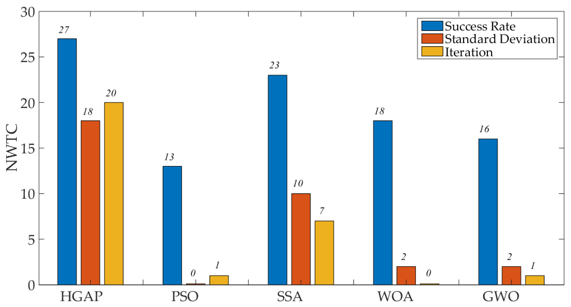
From the results, the HGAP has a 100% success rate for the 27 tested functions, while the other four algorithms all fail on f 5 . In addition, the standard deviation of the HGAP is the smallest in 18 tests, and the convergence speed of the HGAP is the fastest in 18 tests. The number of winning test criteria (NWTC) for each algorithm is counted and shown in Figure 3. A higher NWTC means a better algorithm performance. Note that different algorithms may win the same test criteria. From the results, the HGAP wins all of the test criteria, especially in minimum number of iterations. Most function tests output the final solutions with only a single iteration.
The results show that the HGAP has excellent exploration capabilities with a fewer number of iterations. In addition, since the HGAP does not require gradient information to guide the search, it can avoid falling into the local optimum trap and outputs the globe min/max value more reliably. Hence, the HGAP has more advantage to extract Doppler peaks (max value) from massive raw data in wind measurement.

4.2. Test the Raw Data from the CDWL

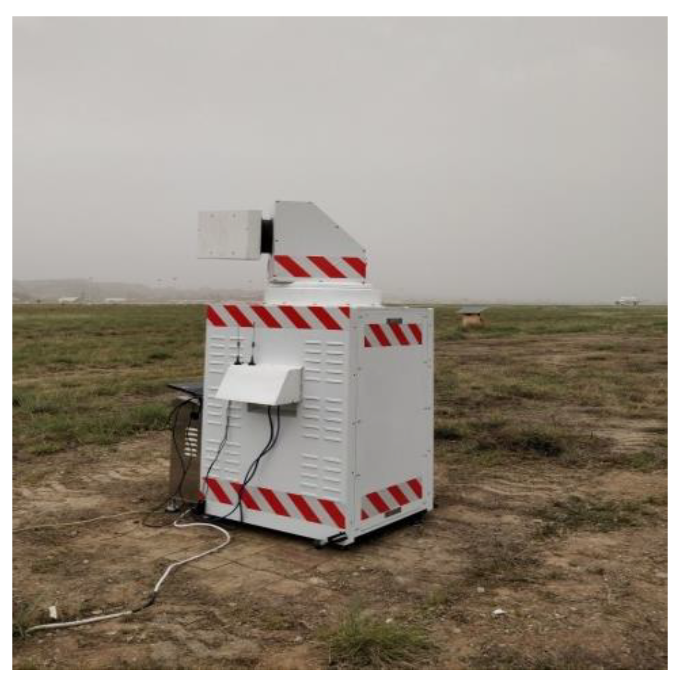
Radial wind measurement was carried out to collect complex wind field data by using a CDWL at Zhong Chuan Airport (36.51 N, 103.62 E), as illustrated in Figure 4. In the experiment, the laser beam emitted by the CDWL was pointed at the runway horizontally.
The key parameters of the CDWL are summarized in Table 3. The detection distance is set at one kilometer with a distance gate of 60 m. In the raw data, it can be seen that some spectra of backscattered signals contain several Doppler peaks. After removing the noise floor, we converted frequency to wind speed according to Formula (1), and the typical spectra are shown in Figure 5.
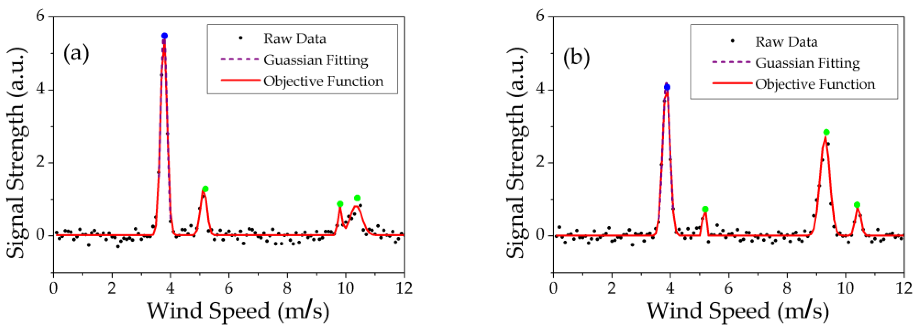
We used the HGAP to process the raw data in Figure 5 and obtained the results as shown in Figure 6. The threshold is set to filter the local maximum value whose strength is not stronger than the noise floor. Figure 6a,b both have four wind speed components, in which the blue dot is the main one and the green dot is the minor. However, traditional Gaussian fitting (GF) just finds the peak of the main component and misses the others. As shown in Table 4, the HGAP not only finds multiple wind speed components quickly but also records the corresponding strength of the backscattered signals. Hence, we can use the spectral centroid method to retrieve the wind speed conveniently, which is more reasonable than the average or the main component. It can be seen that the HGAP is helpful for the analysis of complex wind fields.

5. Conclusions

In this paper, we propose the HGAP, which is the combination of a genetic algorithm and the Powell method, for wind measurement in CDWL. The HGAP has strong ability in global search and fast convergence, which is suitable for massive data analysis. We compared the HGAP with four notable algorithms to solve 27 benchmark functions published by ICEC, and the result shows that our algorithm has great advantages in finding max/min values. In the wind measurement experiments, the HGAP is used to process the raw data from a CDWL, and it also obtained the Doppler peaks efficiently and reliably. The results show that our algorithm not only output wind speed components quickly but also recorded the signal strength of each component. Therefore, the HGAP is helpful for complex wind field analysis and can be further studied for application in more practical models.

Author Contributions

Conceptualization, S.J.; methodology, Z.W. and J.F.; software, Z.W. and D.W.; validation, A.N. and S.L.; formal analysis, J.F.; investigation, S.J.; data curation, Z.W.; writing—original draft preparation, A.N.; writing—review and editing, S.L.; supervision, S.J.; project administration, L.Y.; funding acquisition, S.J. All authors have read and agreed to the published version of the manuscript.

Funding

This research was funded by the Collaborative Innovation Project in Colleges and Universities of Anhui Province grant number GXXT-2020050, and Key Project of Natural Science Research in Colleges and Universities of Anhui Province grant number KJ2020A0125.

Institutional Review Board Statement

Not applicable.

Informed Consent Statement

Not applicable.

Data Availability Statement

Not applicable.

Conflicts of Interest

The authors declare no conflict of interest.

References

  1. Kelley, C.; Herges, T.; Martinez, L.; Mikkelsen, T. Wind turbine aerodynamic measurements using a scanning lidar. J. Phys. Conf. Ser. 2018, 1037, 052014. [Google Scholar] [CrossRef]
  2. Smalikho, I.; Banakh, V.; Holzäpfel, F.; Rahm, S. Method of radial velocities for the estimation of aircraft wake vortex parameters from data measured by coherent Doppler lidar. Opt. Express 2015, 23, 1194–1207. [Google Scholar] [CrossRef] [PubMed] [Green Version]
  3. Käsler, Y.; Rahm, S.; Simmet, R.; Kuhn, M. Wake Measurements of a Multi-MW Wind Turbine with Coherent Long-Range Pulsed Doppler Wind Lidar. J. Atmos. Ocean. Technol. 2010, 27, 1529. [Google Scholar] [CrossRef] [Green Version]
  4. Frehlich, R.; Hannon, S.; Henderson, S. Coherent Doppler lidar measurements of winds in the weak signal regime. Appl. Opt. 1997, 36, 3491. [Google Scholar] [CrossRef]
  5. Huang, J.; Kwok, M.; Chan, P. Wind Shear Prediction from Light Detection and Ranging Data Using Machine Learning Methods. Atmosphere 2021, 12, 644. [Google Scholar] [CrossRef]
  6. Newman, J.; Clifton, A. An error reduction algorithm to improve lidar turbulence estimates for wind energy. Wind Energy Sci. 2017, 2, 77–95. [Google Scholar] [CrossRef] [Green Version]
  7. Eberhard, W. Accuracy of maximum likelihood and least-squares estimates in the lidar slope method with noisy data. Appl. Opt. 2017, 56, 2667–2685. [Google Scholar] [CrossRef]
  8. Agnes, D.; Guillaume, C.; Laurent, L.; Matthieu, V.; Anne, D.; Claudine, B. Long-range wind monitoring in real time with optimized coherent lidar. Opt. Eng. 2016, 56, 031217. [Google Scholar]
  9. Jiang, S.; Feng, J.; Han, F.; Li, Z.; Xiong, D.; Niu, D. Generalized Rayleigh criterion for signal resolution on coherent Doppler wind measurement. Opt. Eng. 2021, 60, 044106. [Google Scholar] [CrossRef]
  10. Lucy, R. Progress towards an HF Radar Wind Speed Measurement Method Using Machine Learning. Remote Sens. 2022, 14, 2098. [Google Scholar]
  11. Williams, C.; Mazoyer, P.; Combrexelle, S. Wind field reconstruction from lidar measurements at high-frequency using machine learning. J. Phys. Conf. Ser. 2018, 1102, 012003. [Google Scholar] [CrossRef]
  12. Sung-Ho, H. Short-term wind speed prediction using Extended Kalman filter and machine learning. Energy Rep. 2021, 7, 1046–4054. [Google Scholar]
  13. Zeng, X.; Guo, W.; Yang, K.; Xia, M. Noise reduction and retrieval by modified lidar inversion method combines joint retrieval method and machine learning. Appl. Phys. B 2018, 124, 238. [Google Scholar] [CrossRef]
  14. Mohandes, M.; Rehman, S. Wind Speed Extrapolation Using Machine Learning Methods and LiDAR Measurements. IEEE Access 2018, 6, 77634–77642. [Google Scholar] [CrossRef]
  15. Newman, J.; Clifton, A. Improving Lidar-Derived Turbulence Estimates for Wind Energy. Wind Energy. Sci. 2016, 22, 072010. [Google Scholar]
  16. Shimada, S.; Kogaki, T.; Takeyama, Y.; Ohsawa, T.; Nakamura, S.; Kawaguchi, K. Accuray of offshore wind measurement using a scanning LiDAR. In Proceedings of the Grand Renewable Energy 2018 Proceedings, Yokohama, Japan, 17–22 June 2018; p. O-We-3-6. [Google Scholar]
  17. Jiang, S.; Sun, D.; Han, F.; Han, Y.; Zheng, J. Performance of continous-wave coherent Doppler Lidar for wind measurement. Curr. Opt. Photonics 2019, 3, 466–472. [Google Scholar]
  18. Holland, J. Adaptation in Natural and Artificial Systems; MIT Press: Cambridge, MA, USA, 1992; pp. 121–140. [Google Scholar]
  19. Powell, M. An efficient method for finding the minimum of a function of several variables without calculating derivatives. Comput. J. 1964, 7, 155–162. [Google Scholar] [CrossRef]
  20. Lin, M.; Chen, W.; Li, B.; Zheng, Y.; Chen, Z. Fast Field Calibration of MIMU Based on the Powell Algorithm. Sensors 2014, 14, 16062–16081. [Google Scholar]
  21. Mirjalili, S.; Lewis, A. The whale optimization algorithm. Adv. Eng. Softw. 2016, 95, 51–67. [Google Scholar] [CrossRef]
  22. Assimi, H.; Jamali, A. A hybrid algorithm coupling genetic programming and Nelder–Mead for topology and size optimization of trusses with static and dynamic constraints. Expert Syst. Appl. 2018, 95, 127–141. [Google Scholar] [CrossRef]
  23. Paul, P.; Moganarangan, N.; Kumar, S.; Raju, R.; Vengattaraman, T.; Dhavachelvan, P. Performance analyses over population seeding techniques of the permutation-coded genetic algorithm: An empirical study based on traveling salesman problems. Appl. Soft Comput. 2015, 32, 383–402. [Google Scholar] [CrossRef]
  24. Okamoto, M.; Nonaka, T.; Ochiai, S.; Tominaga, D. Nonlinear numerical optimization with use of a hybrid genetic algorithm incorporating the modified Powell method. Appl. Math. Comput. 1998, 91, 63–72. [Google Scholar] [CrossRef]
  25. Virtual Library of Simulation Experiments: Test Functions and Datasets. Available online: http://www.sfu.ca/~ssurjano/optimization (accessed on 12 January 2022).
Figure 1. Schematic of the coherent Doppler wind Lidar.
Photonics 09 00802 g001
Figure 2. The process illustration of the HGAP to locate the maximum value point.
Photonics 09 00802 g002
Figure 3. NWTC for each algorithm.
Photonics 09 00802 g003
Figure 4. The CDWL in the field experiment.
Photonics 09 00802 g004
Figure 5. The spectra of radial wind measurements. (a) Spectrum 1; (b) Spectrum 2.
Photonics 09 00802 g005
Figure 6. The spectra processed by the HGAP and the GF. (a) The processing result of spectrum 1; (b) The processing result of spectrum 2.
Photonics 09 00802 g006
Table 1. Benchmark functions published by ICEC 2017.
Function IDFunction NameDimensionGlobe Minimum
f1Ackley100
f2Beale20
f3Bent Cigar100
f4Booth20
f5Bukin20
f6Cross-in-Tray2−2.06
f7Discus100
f8Easom2−1
f9Goldstein-Price2−3
f10Griewank’s100
f11High Conditioned Elliptic100
f12Himmelblau’s20
f13Hölder table2−19.21
f14Levy100
f15Matyas20
f16McCormick2−1.91
f17Michalewicz5−4.69
f18Rastrigin’s100
f19Rosenbrock’s100
f20Schaffer’s F7100
f21Schaffer N.220
f22Schaffer N.420.29
f23Sphere100
f24Styblinski-Tang5−195.83
f25Sum of Different Power100
f26Three-hump camel20
f27Zakharov100
Table 2. The results of the Benchmark functions processing.
Function IdCriteriaHGAPPSOSSAWOAGWO
f1Success rate100%12%100%100%100%
STD4.97 × 10−139.4906.90 × 10−52.69 × 10⁻⁹
Iteration1.996.835.127126.72
f2Success rate100%100%100%100%98%
STD3.92 × 10−328.92 × 10−111.09 × 10−105.19 × 10−70.11
Iteration1.0016.629.0214.8410.24
f3Success rate100%0%100%100%100%
STD6.21 × 10−2239.045.19 × 10−405.56 × 10−66.35 × 10−13
Iteration1.00-7.2475.630.28
f4Success rate100%100%100%100%100%
STD08.20 × 10−111.19 × 10−56.06 × 10−61.45 × 10⁻⁶
Iteration1.0025.0239.8631.3217.78
f5Success rate100%0%0%0%0%
STD2.54 × 10−60.072.96 × 10−160.130.15
Iteration72.86----
f6Success rate100%100%100%100%100%
STD01.05 × 10−109.27 × 10−127.16 × 10−83.41 × 10−8
Iteration1.009.541.265.583.58
f7Success rate100%0%100%100%100%
STD2.95 × 10−266.121.41 × 10−561.10 × 10−94.65 × 10−18
Iteration1.00-7.2254.7417.72
f8Success rate100%100%100%100%100%
STD01.53 × 10−92.48 × 10−85.87 × 10−61.80 × 10⁻⁶
Iteration1.0038.1411.9440.8229.48
f9Success rate100%100%100%100%100%
STD3.14 × 10−161.86 × 10−104.98 × 10−82.33 × 10−51.02 × 10⁻⁴
Iteration1.0027.1830.3235.0421.34
f10Success rate100%0%100%38%4%
STD00.0700.020.04
Iteration82.12-1.3868.6332.50
f11Success rate100%0%100%100%100%
STD4.96 × 10−205.17 × 10−41.69 × 10−382.36 × 10−81.72 × 10−15
Iteration1.00-6.0265.9024.82
f12Success rate100%100%100%100%98%
STD03.60 × 10−104.51 × 10−58.97 × 10−54.85 × 10⁻⁴
Iteration1.0027.7640.6062.7674.22
f13Success rate100%100%100%100%98%
STD3.55 × 10−153.55 × 10−105.25 × 10−62.30 × 10−45.00 × 10⁻³
Iteration1.0025.2236.0073.7886.43
f14Success rate100%100%100%4%44%
STD00.441.44 × 10−60.100.07
Iteration2.6452.942.5098.5094.59
f15Success rate100%100%100%100%100%
STD2.31 × 10−327.79 × 10−121.03 × 10−456.70 × 10−461.47 × 10−43
Iteration1.0011.721.008.403.16
f16Success rate100%78%90%100%100%
STD2.22 × 10−160.020.023.02 × 10−71.79 × 10⁻⁷
Iteration1.0016.748.6615.966.12
f17Success rate100%18%0%0%2%
STD3.97 × 10−160.370.460.460.26
Iteration81.6861.11--100
f18Success rate100%0%100%74%22%
STD08.7101.503.06
Iteration1.90-4.727.153.50
f19Success rate100%0%100%0%0%
STD8.23 × 10−24390.472.26 × 10−797.876.15
Iteration1.00-6.00--
f20Success rate100%64%100%48%26%
STD5.46 × 10−324.39 × 10−36.67 × 10−160.010.06
Iteration1.0033.031.0288.1789.31
f21Success rate100%100%100%100%100%
STD0 4.24 × 10 13 000
Iteration17.2818.321.0017.685.26
f22Success rate100%100%100%100%100%
STD1.76 × 10−71.17 × 10−81.20 × 10−41.33 × 10−61.39 × 10−6
Iteration75.5020.9226.0219.465.94
f23Success rate100%100%100%100%100%
STD1.78 × 10−268.42 × 10−76.03 × 10−421.40 × 10−89.80 × 10−17
Iteration1.0071.061.8060.0620.94
f24Success rate100%34%98%6%32%
STD011.948.56 × 10−46.314.24
Iteration50.4247.1125.6787.6595.60
f25Success rate100%28%100%100%100%
STD1.15 × 10−321.40 × 10−91.13 × 10−381.02 × 10−132.94 × 10⁻³⁰
Iteration1.0083.501.4056.9818.14
f26Success rate100%100%100%100%100%
STD2.25 × 10−312.76 × 10−124.44 × 10−396.08 × 10−442.91 × 10−70
Iteration1.0015.081.549.263.20
f27Success rate100%0%100%100%100%
STD1.15 × 10−259.28 × 10−92.19 × 10−526.19 × 10−91.17 × 10−17
Iteration1.0050.162.7654.2616.08
Table 3. Key parameters of the CDWL.
ItemParametersValue
LaserWavelength1547 nm
Line width4 kHz @ 1547 nm
Pulse energy150 uJ
Pulse width200 ns
Pulse repetition frequency10 kHz
TelescopeEffective aperture150 mm
Balanced detectorResponsiveness0.95 A/W
3-dB bandwidth250 MHz
A/D converterSample rate500 MHz
Table 4. The measurement result of Figure 6.
FigureComponentSpeed
(m/s)
Strength
(a.u.)
Speed Measured by GF (m/s)Speed Measured by HGAP(m/s)
Figure 6aMain3.816.133.795.56
Minor 15.151.52
Minor 29.821.06
Minor 310.351.43
Figure 6bMain3.944.763.916.71
Minor 15.201.88
Minor 29.283.45
Minor 310.401.93
Publisher’s Note: MDPI stays neutral with regard to jurisdictional claims in published maps and institutional affiliations.