Article

Toward Real-Time Giga-Voxel Optoacoustic/Photoacoustic Microscopy: GPU-Accelerated Fourier Reconstruction with Quasi-3D Implementation

1
Institute of Applied Physics RAS, 603950 Nizhny Novgorod, Russia
2
Institute of Applied Physics, University of Bern, 3012 Bern, Switzerland
*
Author to whom correspondence should be addressed.
These authors contributed equally to this work.
Photonics 2022, 9(1), 15; https://doi.org/10.3390/photonics9010015
Submission received: 29 November 2021 / Revised: 17 December 2021 / Accepted: 21 December 2021 / Published: 29 December 2021
(This article belongs to the Special Issue Advances in Modern Photonics)

Abstract

:
We propose a GPU-accelerated implementation of frequency-domain synthetic aperture focusing technique (SAFT) employing truncated regularized inverse k-space interpolation. Our implementation achieves sub-1s reconstruction time for data sizes of up to 100 M voxels, providing more than a tenfold decrease in reconstruction time as compared to CPU-based SAFT. We provide an empirical model that can be used to predict the execution time of quasi-3D reconstruction for any data size given the specifications of the computing system.

1. Introduction

Raster-scan optoacoustic (OA) angiography is a hybrid technique allowing for the imaging of blood vessels using focused ultrasonic detectors due to local, laser-generated thermoelastic expansion of hemoglobin [1]. High optical absorption by hemoglobin near the 532 nm laser wavelength, and wideband ~100 MHz ultrasound detectors provide commercial OA microscopes (OAMs) [2,3] with the ability to perform volumetric optoacoustic angiography of a ~6 × 6 × 3 mm3 volume with mega-voxel resolution in several minutes. Modern laboratory OAM prototypes equipped with higher-powered lasers and faster-scanning electronics [4,5] provide giga-voxel images within the same scanning time.
To improve the lateral resolution of OAM angiography above or below the focal plane (Figure 1), the acquired OAM datasets require processing by reconstruction algorithms utilizing the synthetic aperture focusing technique (SAFT) [6]. Similar to other mechanical scanning techniques (such as cross-sectional CT and MRI), OAM SAFT reconstruction algorithms are typically not applied to full-3D datasets (XYZ), but to sequential 2D datasets (XZ) called B-scans, which are obtained in the course of mechanical zig-zag scanning. While XZ-reconstructions can often be done in parallel with B-scan acquisition, YZ-reconstructions usually require prior compensation for motion artifacts [7] characteristic of most in vivo subjects due to their respiration and heartbeat during the scanning.
Although sequential 2D reconstruction is computationally less complex than its full-3D counterparts [8], the 2D SAFT reconstruction algorithms performed in the time domain (TD) may require relatively large numbers of computations, especially if performed using standard central processing units (CPUs). For example, 2D realization of the SAFT-TD reported in [9] and performed on a standard CPU could require more than one minute even for mega-voxel datasets.
Significant reduction in the computation time was achieved by performing two-dimensional SAFT reconstruction in the frequency domain (FD) [10,11,12]. The 2D fast Fourier transform (FFT) simplifies the computational complexity by the factor [ N X × N Z ] / l o g 2 [ N X × N Z ] , thus providing the performance necessary for online reconstruction of mega-voxel resolution at the speed of volume scanning. However, real-time SAFT-FD processing of giga-voxel datasets still remained an unmet challenge.
This manuscript focuses on the comparison of algorithms for accelerated reconstruction of large volumes of OAM data using parallel computing [13]. Since most SAFT-FD calculations are arithmetically simple and not co-dependent, they fit well with the architecture of modern graphics processing units (GPUs), which are optimized for parallel computations. The algorithm implemented in this manuscript is described in [10].

2. Materials and Methods

2.1. GPU-FD Accelerated Reconstruction

The GPU-FD algorithm used in this study is based on the SAFT-FD algorithm developed in [10]. In summary, this algorithm relates the spatial frequencies ( k X , k Z ) of the discrete Fourier transform of the to-be-reconstructed image to the spatial/time frequencies ( k X , k t ) of the discrete Fourier transform of the B-scan. This is nearly a one-to-one relation given that k t is a function of the modulus of ( k X , k Z ) , which is the reason why the computational complexity of SAFT-FD is dominated by the discrete FT. Due to the discreteness of the frequency grids, however, crosstalk exists between different k t , and interpolation is needed to invert this relation. In [10], complex-valued interpolation weights were determined based on a regularized pseudo-inverse approach. Previous work [10] also showed that the number of interpolation nodes ( k X , k Z ) per ( k X , k Z ) can be truncated to a small value α (typically 5 to 10) without a significant change to image quality, and that this is independent of the total grid sizes.
A simplified block diagram of the GPU-FD algorithm implemented in MATLAB is shown in Figure 2. While the initialization of data-independent parameters is performed on the CPU, processing of the data is performed as parallelized tasks on the GPU. The data-independent parameters are: the definition of interpolation node indices, interpolation weights, and a filter matrix for combined processing of focal plane selection; compensation of limited angle detection; and Hilbert transform.
The implemented pipeline consists of the simplest arithmetic operations with the exception of forward/inverse FFT 2D functions (Figure 2) [14]. The number of spatial frequencies ( k X , k Z ) is chosen to be identical to the number of pixels N X × N Z . However, in the case of using zero padding, the number of frequencies would be double the number of pixels in both the X- and the Z-dimensions.
While the characteristics of the GPU-FD algorithm can be determined according to certain classifications [15], the following advantages of the pipeline (Figure 2) should be mentioned: First, GPU-FD realization has massive (>75%) data parallelism. Next, the number of threads exceeds the number of spatial frequencies, and therefore the thread count is relatively high. Further, the number of synchronizations used for one B-scan after each arithmetic operation between the FFT 2D and the inverse FFT 2D is relatively small (6 pcs). Finally, the implemented pipeline (Figure 2) does not have branch divergence.
The minimum memory required for implementation of the GPU-FD algorithm is:
2 ( α + 1 ) N X × N Z , where N Z 2 Δ Z / A R where N Z is the required number of points in the A-scan defined by the ultrasound probing depth Δ Z and the axial resolution (AR) of the OAM system (usually N Z ~ 200), and N z 2 Δ X / L R is the required number of scanning lines in B-scan defined by the scanning range Δ X and the lateral resolution (LR) of the detector (usually N X > 200 ). For enhanced OA image quality, oversampling by a factor of two, as dictated by the Nyquist sampling theorem, can often be replaced by a factor of five, leading to N Z = 5 Δ Z / A R and N X = 5 Δ X / L R evaluations. For enhanced reconstruction quality within the depth range Δ Z , it is also important that the acquisition range is wider than Δ Z , so that the diagonals corresponding to the maximum receiving angles of the detector are fully covered. However, for simplicity we will assume that the number of axial pixels N Z in the raw and the reconstruction volumes is the same throughout the manuscript.
The computation time T e x e of the GPU-FD reconstruction algorithm can be estimated as:
T e x e = T 0 + N Y × T r e c
where T 0 is the execution time of the preliminary preparation of indices and coefficients, T r e c is the execution time of the 2D reconstruction per B-scan (Figure 2) and N Y is the number of B-scans.
The algorithmic complexity of both the preparation T 0 and the reconstruction T r e c stages are dependent on the number of spatial frequencies in the X - and Z -dimensions. In the considered case (Figure 2) of minimally required spatial sampling periods ( 2 π / N X , 2 π / N Z , the number of spatial frequencies is equal to the number of pixels in each B-scan O ( [ N X × N Z ] ) . However, denser linear sampling in the Fourier domain quadratically increases the algorithmic complexity. For example, a factor-of-two zero-padding quadruples the number of spatial frequencies with respect to the original number of pixels.
The reconstruction stage primarily depends on the FFT execution, with a computational complexity of O ( N X × N Z × l o g 2 [ N X × N Z ] ) . In the case of fully parallelized execution of the algorithm [16], the execution time can be approximated as:
T e x e = A · N X × N Y × N Z p G P U · f G P U + B · N X × N Y × N Z p G P U · f G P U · l o g 2 ( N X × N Z ) + C · N X p C P U · f C P U
where f G P U , C P U are the clock speeds; p G P U , C P U are the effective number of processing cores (cores in the case of CPU; stream processors/CUDA cores in the case of GPU); and the parameters A, B and C are scaling factors dependent on the algorithm implementation (and independent of the computing system configuration and the data volume).

2.2. Experimental Data

A fiber-based version [17] of dark-field OAM [18] with L R = 50 µ m was used to perform a Δ X = Δ Y = 8 m m lateral OA scan of an experimental tumor CT-26 [19] with δ X = δ Y = 10 µ m scanning steps at a laser wavelength of 532 nm. The superficial tumor vasculature was aligned with a 6.7 ± 0.75 mm depth-of-field, a custom-made [20,21], 6.7 ± 0.75 mm depth-of-field, wideband 1–100 MHz spherical ultrasonic PVDF detector. Each OA A-scan with 10.24 µs duration was converted to 2048 samples by a 16-bit Razor16 (GaGe, Lockport, IL, USA) digitizer at a sampling rate of 200 MHz. The acquired XYZ-volume was then cropped above and below the focal plane within the 1 µs time interval corresponding to a depth range of ~6.7 ± 0.75 mm. The initial size of the raw OA dataset thus contained { N X × N Y × N Z = 800 × 800 × 200 = 128 M } voxels. To evaluate the voxel-count dependent characteristics of the GPU-FD algorithm, OAM angiograms with a larger/smaller number of voxels were synthesized by resampling the original OAM angiogram.

3. Results and Discussion

Figure 3 shows the maximum intensity projections (MIP) of a raw angiographic image (128 M voxels) and the procedure of consecutive application of the GPU-FD algorithm (Figure 2) in two perpendicular orientations, leading to quasi-3D reconstruction. While the first reconstruction in the XZ-plane improves the resolution in the X-direction, the second reconstruction in the YZ-plane also improves the resolution in the Y-direction, resulting in the OA MIP angiogram representing the vascular tumor microenvironment down to 50-micron resolution in both the X- and Y-directions.
Since the mouse was immobilized using gas anesthesia, and the thigh with the tumor located on it was fixed against the OAM immersion chamber, the mouse respiratory movements did not have a visible effect on the image quality in the Y-direction. In the presence of motion artifacts, motion compensation algorithms [22] would have to be applied between XZ- and YZ-reconstruction.
Figure 4 compares the execution times of the CPU-TD [9] and CPU-FD [11], and the GPU-based counterpart of the latter. The numerical tests evaluating voxel-dependent execution time for different reconstruction algorithms were performed on different processing units characterized by different clock speeds and different thread counts (Table 1).
In comparison to the CPU-FD reconstruction (blue circles in Figure 4), the decrease in execution time for the GPU-FD algorithm (green circles in Figure 4) is more than one order of magnitude over the whole range of considered OAM data volumes. While the largest data volume (4.2G voxels) required ~7 h execution time for the CPU-TD algorithm and ~13 min for the CPU-FD algorithm, the accelerated GPU-FD algorithm obtained the same reconstructed 3D-dataset in less than 40 s (Figure 4). A more recent GPU (Nvidia GeForce RTX 3090) executed the GPU-FD algorithm for the standard 128M-voxel data volume in less than a second.
The execution times measured for different data sets using three different GPUs are plotted as solid curves in Figure 5. The dotted curves were fitted according to Equation (2), thus providing empirical evaluation of constants A, B and C.
The precise analytical prediction of the reconstruction time T a ( f , p , N X , N Y , N Z ) is difficult due to the uncertainty in p e f f , which is an estimate of the effective number of cores participating in the computation. This is necessary because a large number of cores can only be used efficiently if the voxel count is comparatively large. While Formula (2) remains applicable in the case of large datasets N X × N Z p , leading to all cores becoming involved ( p e f f / p = 1 ), in the case of relatively small datasets N X × N Z < p not every core can be utilized ( p e f f / p < 1 ), thus leading to lower GPU performance. The effective number of cores p e f f is estimated to increase linearly with the voxel count up to a saturation point p r a t i o , where p e f f / p = 1 . To take into account voxel-dependence of the p e f f / p ratio, the initial model (2) can be expanded to the following, where p r a t i o , the saturation point, is an additional fitting parameter:
T e x e = A · N X × N Y × N Z f G P U · p e f f + B · N X × N Y × N Z f G P U · p e f f · l o g 2 ( N X × N Z ) + C · N X f C P U · p C P U
p e f f = { p , i f ( N X × N Z ) / p > p r a t i o ( N X × N Z ) / p r a t i o , i f ( N X × N Z ) / p < p r a t i o
A = 2.3 × 10 3 , B = 1.1 × 10 1 , C = 5.4 × 10 4 , p r a t i o = 7.8
The expanded model as described in Formula (3) is thus capable of providing an accurate estimation of the GPU-FD algorithm computation time for any dataset size based on the technical specifications of a given computing system.
In comparison to the 3D-SAFT developed in [13], our quasi-3D implementation reaches equal performance even for the relatively small data size the authors provided as an example. This comparison is also true for a full-3D implementation of GPU-FD, due to the independence of the FFT algorithm on the dimensionality of the data. It is important to note, however, that our implementation does not employ the same level of optimization, instead prioritizing ease of development and platform-independence over performance by keeping the implementation purely as MATLAB code. Implementation as an OpenCL or CUDA kernel instead, as was done in [13], is expected to yield a significant performance advantage.
While this manuscript focuses solely on the application in optoacoustic microscopy, the same algorithm for quasi-3D reconstruction can also be used for tomography. For 2D tomography based on a linear detector array, the cyclic part of the pipeline (Figure 2) can be directly applied to individual B-scans. Since the speed of operation in 2D mode can be several orders of magnitude higher than in quasi-3D mode, 2D real-time reconstruction at more than 100 Hz B-scan acquisition rates is feasible.

4. Conclusions

The proposed GPU-accelerated implementation of a frequency-domain, 2D synthetic aperture focusing technique shows great promise in speeding up optoacoustic image reconstruction in both 2D and 3D. The developed numerical methods reduce the time for quasi-3D processing of giga-voxel optoacoustic data volumes to several seconds. To study the applicability of the developed algorithm for solving certain practical problems, it is advisable to use the empirical model proposed in this manuscript, which allows estimating the expected reconstruction time depending on the volume of processed data and the parameters of the computing system.

Author Contributions

Conceptualization, V.P., F.S., M.J., M.F. and P.S.; Software, A.K. (Andrey Kovalchuk), A.K. (Aleksandr Khilov), V.P., F.S. and P.S.; Investigation, F.S., P.S. and M.J.; Resources, M.J. and P.S.; Visualization, K.P., A.K. (Alexey Kurnikov) and P.S.; Writing—original draft, P.S. and F.S.; Writing—review and editing, F.S., P.S., M.F. and M.J. Funding acquisition, P.S. and M.J. All authors have read and agreed to the published version of the manuscript.

Funding

The development of the GPU-accelerated (GPU-FD) version of the reconstruction algorithm was supported by the Centre of Excellence “Center of Photonics” funded by the Ministry of Science and High Education of the Russian Federation, agreement No. 075-15-2020-906. The evaluation of the developed algorithms has been funded by the Swiss National Science Foundation, under Project No. 205320-179038.

Institutional Review Board Statement

The animal study protocol was approved by the Ethics Committee of Lobachevsky State University of Niznhny Novgorod (Protocol No 47, 22.10.2020).

Data Availability Statement

The code for the GPU-FD algorithm and the data used in this research are available from Pavel Subochev and Florentin Spadin upon reasonable request.

Acknowledgments

The authors are thankful to Anna Orlova for assistance with the experimental animal.

Conflicts of Interest

The authors declare no conflict of interest.

References

  1. Yao, J.; Wang, L.V. Photoacoustic microscopy. Laser Photonics Rev. 2013, 7, 758–778. [Google Scholar] [CrossRef] [PubMed]
  2. Haedicke, K.; Agemy, L.; Omar, M.; Berezhnoi, A.; Roberts, S.; Longo-Machado, C.; Skubal, M.; Nagar, K.; Hsu, H.-T.; Kim, K. High-resolution optoacoustic imaging of tissue responses to vascular-targeted therapies. Nat. Biomed. Eng. 2020, 4, 286–297. [Google Scholar] [CrossRef] [PubMed]
  3. Saijo, Y.; Ida, T.; Iwazaki, H.; Miyajima, J.; Tang, H.; Shintate, R.; Sato, K.; Hiratsuka, T.; Yoshizawa, S.; Umemura, S. Visualization of skin morphology and microcirculation with high frequency ultrasound and dual-wavelength photoacoustic microscope. In Photons Plus Ultrasound: Imaging and Sensing 2019; International Society for Optics and Photonics: Bellingham, WA, USA, 2019; p. 108783E. [Google Scholar] [CrossRef]
  4. Hofmann, U.A.; Rebling, J.; Estrada, H.; Subochev, P.; Razansky, D. Rapid functional optoacoustic micro-angiography in a burst mode. Opt. Lett. 2020, 45, 2522–2525. [Google Scholar] [CrossRef] [PubMed]
  5. Baik, J.W.; Kim, J.Y.; Cho, S.; Choi, S.; Kim, J.; Kim, C. Super wide-field photoacoustic microscopy of animals and humans in vivo. IEEE Trans. Med. Imaging 2019, 39, 975–984. [Google Scholar] [CrossRef] [PubMed]
  6. Li, M.-L.; Zhang, H.F.; Maslov, K.; Stoica, G.; Wang, L.V. Improved in vivo photoacoustic microscopy based on a virtual-detector concept. Opt. Lett. 2006, 31, 474–476. [Google Scholar] [CrossRef] [PubMed] [Green Version]
  7. Schwarz, M.; Garzorz-Stark, N.; Eyerich, K.; Aguirre, J.; Ntziachristos, V. Motion correction in optoacoustic mesoscopy. Sci. Rep. 2017, 7, 10386. [Google Scholar] [CrossRef] [PubMed] [Green Version]
  8. Lutzweiler, C.; Razansky, D. Optoacoustic imaging and tomography: Reconstruction approaches and outstanding challenges in image performance and quantification. Sensors 2013, 13, 7345–7384. [Google Scholar] [CrossRef] [PubMed] [Green Version]
  9. Perekatova, V.V.; Kirillin, M.Y.; Turchin, I.V.; Subochev, P.V. Combination of virtual point detector concept and fluence compensation in acoustic resolution photoacoustic microscopy. J. Biomed. Opt. 2018, 23, 091414. [Google Scholar] [CrossRef] [PubMed] [Green Version]
  10. Jaeger, M.; Schüpbach, S.; Gertsch, A.; Kitz, M.; Frenz, M. Fourier reconstruction in optoacoustic imaging using truncated regularized inverse k-space interpolation. Inverse Probl. 2007, 23, S51. [Google Scholar] [CrossRef]
  11. Spadin, F.; Jaeger, M.; Nuster, R.; Subochev, P.; Frenz, M. Quantitative comparison of frequency-domain and delay-and-sum optoacoustic image reconstruction including the effect of coherence factor weighting. Photoacoustics 2020, 17, 100149. [Google Scholar] [CrossRef] [PubMed]
  12. Jin, H.; Liu, S.; Zhang, R.; Liu, S.; Zheng, Y. Frequency domain based virtual detector for heterogeneous media in photoacoustic imaging. IEEE Trans. Comput. Imaging 2020, 6, 569–578. [Google Scholar] [CrossRef]
  13. Liu, S.; Feng, X.; Gao, F.; Jin, H.; Zhang, R.; Luo, Y.; Zheng, Y. Gpu-accelerated two dimensional synthetic aperture focusing for photoacoustic microscopy. APL Photonics 2018, 3, 026101. [Google Scholar] [CrossRef]
  14. Puchała, D.; Stokfiszewski, K.; Yatsymirskyy, M.; Szczepaniak, B. Effectiveness of fast fourier transform implementations on gpu and cpu. In Proceedings of the 2015 16th International Conference on Computational Problems of Electrical Engineering (CPEE), Lviv, Ukraine, 2–5 September 2015; pp. 162–164. [Google Scholar] [CrossRef]
  15. Smistad, E.; Falch, T.L.; Bozorgi, M.; Elster, A.C.; Lindseth, F. Medical image segmentation on gpus—A comprehensive review. Med. Image Anal. 2015, 20, 1–18. [Google Scholar] [CrossRef] [PubMed]
  16. Chu, E.; George, A. Inside the FFT Black Box: Serial and Parallel Fast Fourier Transform Algorithms; CRC Press: Boca Raton, FL, USA, 1999. [Google Scholar]
  17. Subochev, P. Cost-effective imaging of optoacoustic pressure, ultrasonic scattering, and optical diffuse reflectance with improved resolution and speed. Opt. Lett. 2016, 41, 1006–1009. [Google Scholar] [CrossRef] [PubMed]
  18. Maslov, K.; Stoica, G.; Wang, L.V. In vivo dark-field reflection-mode photoacoustic microscopy. Opt. Lett. 2005, 30, 625–627. [Google Scholar] [CrossRef] [PubMed]
  19. Orlova, A.; Sirotkina, M.; Smolina, E.; Elagin, V.; Kovalchuk, A.; Turchin, I.; Subochev, P. Raster-scan optoacoustic angiography of blood vessel development in colon cancer models. Photoacoustics 2019, 13, 25–32. [Google Scholar] [CrossRef] [PubMed]
  20. Kurnikov, A.A.; Pavlova, K.G.; Orlova, A.G.; Khilov, A.V.; Perekatova, V.V.; Kovalchuk, A.V.; Subochev, P.V. Broadband (100 kHz–100 MHz) ultrasound PVDF detectors for raster-scan optoacoustic angiography with acoustic resolution. Quantum Electron. 2021, 51, 383. [Google Scholar] [CrossRef]
  21. Subochev, P.V.; Prudnikov, M.; Vorobyev, V.; Postnikova, A.S.; Sergeev, E.; Perekatova, V.V.; Orlova, A.G.; Kotomina, V.; Turchin, I.V. Wideband linear detector arrays for optoacoustic imaging based on polyvinylidene difluoride films. J. Biomed. Opt. 2018, 23, 091408. [Google Scholar] [CrossRef] [PubMed] [Green Version]
  22. Ron, A.; Davoudi, N.; Deán-Ben, X.L.; Razansky, D. Self-gated respiratory motion rejection for optoacoustic tomography. Appl. Sci. 2019, 9, 2737. [Google Scholar] [CrossRef] [Green Version]
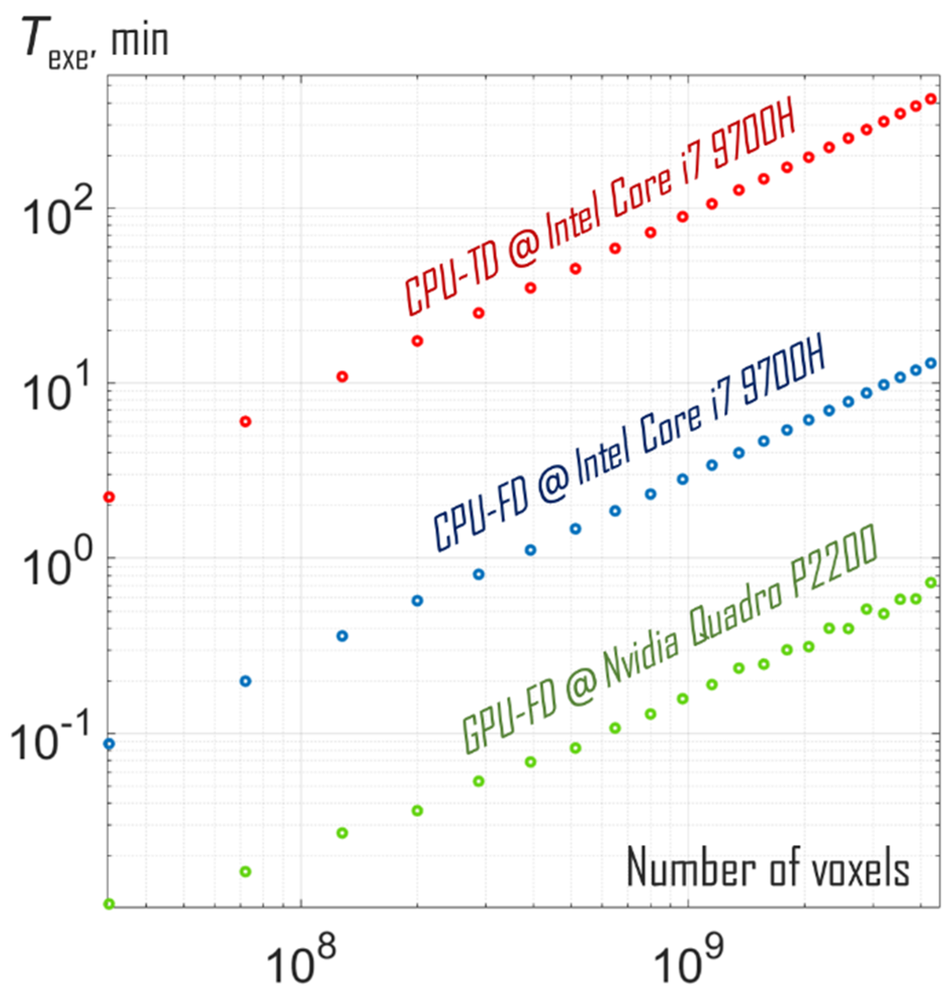
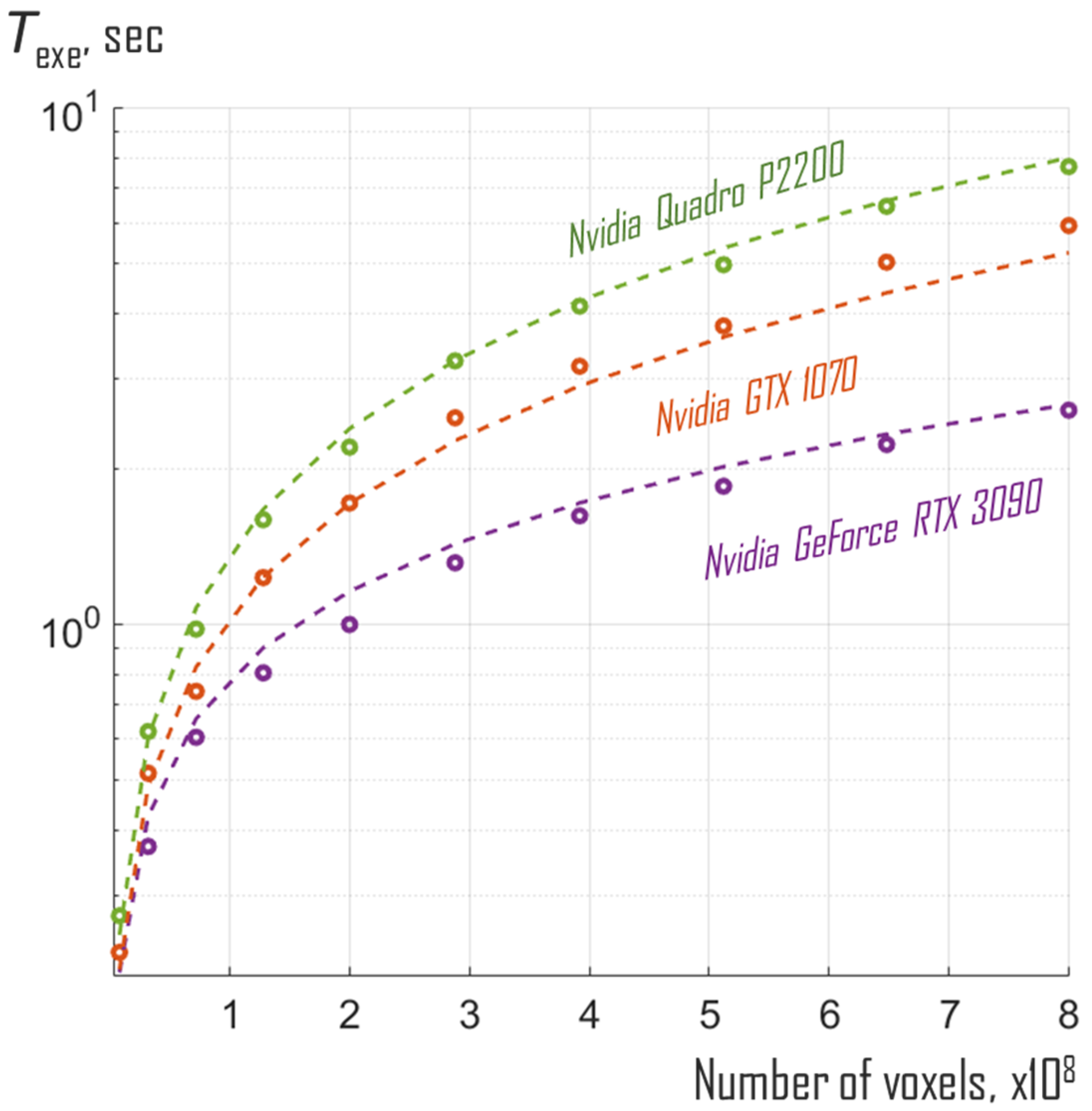
Figure 1. Raster-scan OAM angiography with simultaneous acquisition and SAFT reconstruction.
Photonics 09 00015 g001
Figure 2. Block diagram of the GPU-FD algorithm. Represented in the center are pre-processed matrices containing the reconstruction indices (with α denoting the number of interpolation nodes), the complex interpolation weights used for interpolation and the filter matrix.
Photonics 09 00015 g002
Figure 3. Sequential implementation of GPU-FD algorithm in XZ/YZ planes.
Photonics 09 00015 g003
Figure 4. Execution times for different algorithms and different data volumes.
Photonics 09 00015 g004
Figure 5. Execution times for different voxel counts and different processing units: experimental data (markers); and theoretical data (dotted curves).
Photonics 09 00015 g005
Table 1. Execution times for 128M-voxel OAM data volume using different processing units.
Processing UnitClock SpeedNumber of CoresExecution Time, s
CPU-TDCPU-FDGPU-FD
Nvidia GeForce RTX 30901.7 GHz10,496n/an/a0.8
Nvidia GTX 10701.7 GHz1920n/an/a1.2
Nvidia Quadro P22001.5 GHz1280n/an/a1.6
Intel Core i7 9700H4.7 GHz870022n/a
Publisher’s Note: MDPI stays neutral with regard to jurisdictional claims in published maps and institutional affiliations.

