1. Introduction
Photoacoustic computed tomography (PACT) combines the merits of high ultrasound penetration and high optical contrast in a single modality, and is capable of high-resolution structural and functional imaging in biological tissue beyond the depth of optical diffusion limit [
1,
2,
3]. To date, it has been widely employed in a variety of biomedical applications [
3,
4,
5], such as brain vascular network visualization [
6], small animal whole body imaging [
7], breast cancer detection [
8], and finger joint imaging [
9].
In PACT, wide illumination over the whole sample is used, and ultrasound signals are collected by scanning the transducer around the sample or using transducer arrays, assuming that each transducer element covers the whole image domain. Then, an image reconstruction method is utilized to restore the light absorption distribution of the whole region at once [
6,
9,
10,
11].
The scanning geometry of PACT can be linear, circular, and spherical, or the combinations of the above geometries. Compared with linear scanning [
11], the circular (for 2D imaging) [
9] and spherical (for 3D imaging) [
10] scanning can provide better imaging quality for covering a more complete angle of views of the target. Besides the optimization of the scanning geometry, a fast and accurate image reconstruction algorithm is the key to improve the quality of the reconstructed images [
12].
Among various PACT reconstruction algorithms, the back-projection (BP) method is mostly employed due to its good stability and low computation cost [
13,
14,
15]. However, most of the current PAT reconstruction algorithms including the BP method simply model the ultrasound transducer as point detectors, which however are usually planar and can reach several millimeters in size in circular or spherical scanning [
16,
17]. This geometry miss-model of the transducer detection surface in the reconstruction algorithm leads to the “finite aperture effect” [
17,
18,
19]. Due to this effect, in PACT based on circular/spherical scanning, when the target is far away from the rotation center, the lateral resolution will deteriorate rapidly. Theoretical analysis shows that the lateral resolution is proportional to the distance from the rotation center, and equal to the transducer aperture size on the transducer detection surface [
19].
To date, several methods have been proposed to improve this elongated lateral resolution. A large number of researchers employ focus transducers in circular-scanning-based PAT with a virtual-point-detector method [
20,
21], but these methods are reported to be unable to reliably reconstruct the high frequency part of the target [
22]. Model-based method have been proposed to incorporate the transducer geometries to overcome the “finite aperture effect”, but the computational cost is too high to be applied on routing practice imaging. Deconvolution as an image post-processing method can also potentially improve the lateral resolution, but as a typical inverse method, it can induce strong image noises [
23,
24,
25,
26]. Therefore, new PACT reconstruction algorithms are still needed to overcome the influence of the finite transducer sized in circular/spherical-scanning-based PACT.
Essentially, the decrease of the lateral resolution is due to the spatial averaging of the photoacoustic signal over the transducer aperture, which makes the spatial impulse response (SIR) of a finite-sized transducer different from an ideal point detector [
27]. Therefore, in this work we propose a novel BP method that is based on the fast calculation of SIR related parameters. Here, the lateral resolution improvement with this novel SIR based BP (SIR-BP) method was demonstrated with both simulations and phantom experiments in 2D circular-scanning-based PAT. Results show that the computational time of this SIR-BP method was as short as the conventional BP method.
2. Materials and Methods
2.1. Reconstruction Algorithms
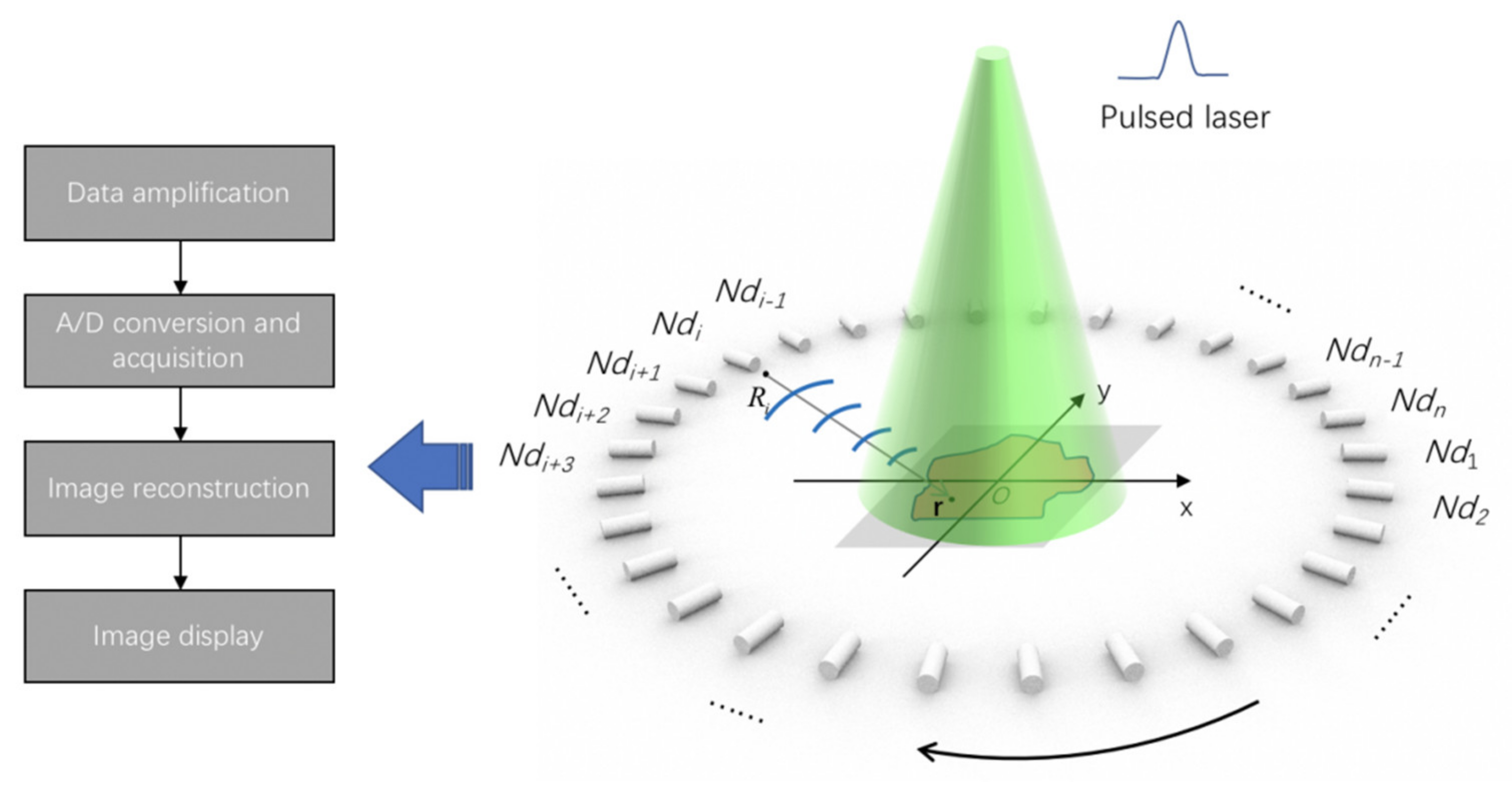
Figure 1 shows the schematic of a conventional 2D circular PAT scan. Aerial illumination is given on the target with an infinitely short, pulsed laser. The generated photoacoustic signal
is collected at a total of
transducer positions around the target. If the acoustic velocity is assumed to be homogenous, there is analytical solutions to the optical absorption distribution
in the image domain, which can be given as the following universal BP equation by Xu and Wang [
14],
Here, is the received acoustic signal by the -th transducer at . The coefficient is to weight the contributions from different transducers based on their angular coverage with respect to the target.
The above BP methods models the transducer as an ideal point detector. However, in most current PAT systems the transducer aperture is mostly planar, and the aperture size can be of several millimeters. If considering the effect of the transducer aperture, the actual received photoacoustic pressure
at the transducer position
should be written as the follows integral over the transducer detection surface
SHere,
r is the position of the photoacoustic source, and
is the position on the transducer. Therefore,
It can be seen that is greatly affected by the SIR due to the spatial integral over the transducer detection surface. Thus, the analytical solution in (1) becomes invalid in this case. The result is that the image will be blurred in the regions far from the rotation center due to an elongated lateral resolution, which is also known as the “finite aperture effect”. From a deeper point of view, the SIR determines the flight time from the acoustic point source (or the time delay), as well as the spatial-dependent sensitivity. Because these two factors are different in the SIR of a finite-sized transducer and the SIR of an ideal point detector, they must be reflected in the image reconstruction method.
Therefore, we propose to replace the time delay and the weighting factor in (1) with SIR related expressions, which is the basis of our proposed SIR-BP method in this work. Firstly, in the conventional BP method, the time delay is expressed as
. In the SIR-BP method, considering the finite transducer aperture, the time delay is a function of the relative distance from the transducer to the acoustic source
, which can be termed to be
. Thus, (1) becomes
Here, the weighting factor is not considered and we assume signals collected at different transducer positions give equal contributions. We call this kind of time delay compensation-based BP method to be the TDC-BP method.
Furthermore, in the conventional BP method given by (1), the weighting factor
is set to be constant. However, because the acoustic field or the sensitivity of the finite-sized transducer is spatially dependent, and it is also a function of the vector
, we termed the weighting factor to be
. Then, the SIR-BP method obtained from (4) can be written as follows
Here, the weighting factor is set to be the reciprocal of the amplitude of the
SIR waveform
, as in (6)
2.2. SIR-Related Time-Delay and Weighting Factor Expressions
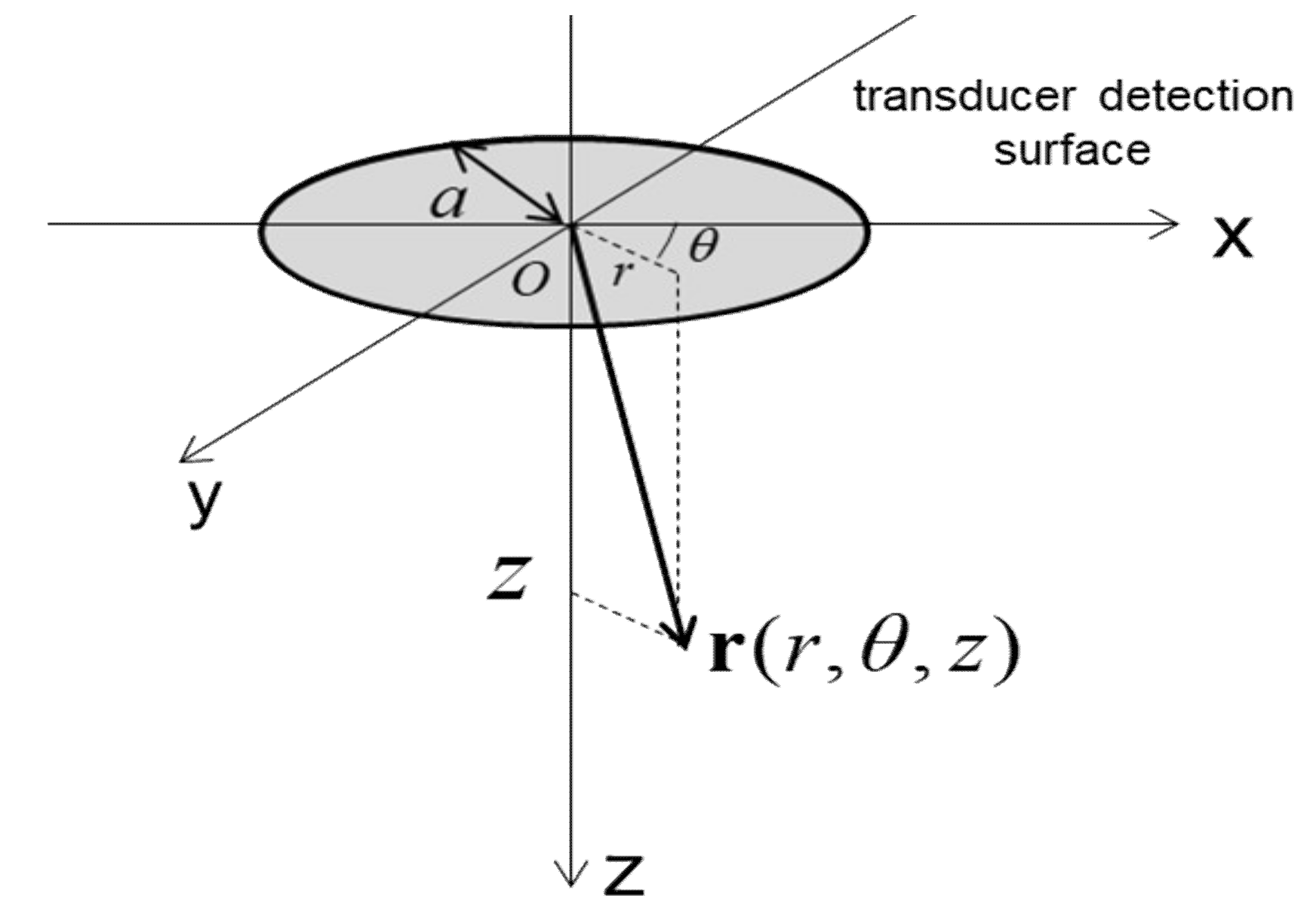
Next, we have to find the expressions based on the SIR for and . As in (3), the SIR is calculated to be the integral over the transducer’s detection surface. Because most planar transducers’ detection surface is circular, the SIR can be obtained analytically in the cylindrical coordination due to the symmetry.
As shown in
Figure 2, we set the detection surface of the transducer in the z = 0 plane and take its center to be the origin of the coordinates. The detection surface of the transducer has a radius of
, and the laser pulse width is sufficiently small. Then, for an observation point
, the
SIR is
There are analytical expressions of the integral of (7), which can be derived in two different cases depending on whether the acoustic point source is within the aperture of the disk in the x-y plane or not [
28], as shown in (8)
Here,
t1 and
t2 correspond to the flight time from the edges of the disk closest and farthest to the photoacoustic source position
respectively, so that
In this work, we take the peak arrival time of the
SIR waveform to be
. From (8), we can see that the analytical expression of this time delay can also be divided into two cases:
Additionally, the analytical expression for the amplitude of the SIR waveform
can be obtained from (10) after dropping the constant of
, so that
The final reconstruction results were given by taking (10) and (11) into (7) in SIR-BP, or just taking (10) into (6) in TDC-BP.
2.3. Numerical Simulations
Point targets imaging simulations were carried out. A planar transducer was employed, which had a bandwidth of 70% and a diameter of 5 mm, and the distance from the transducer to the rotation center was 25 mm. There were 720 detectors in the full scan with an angular interval of 0.5 degree. In these simulations, different transducer central frequencies was tested, which were 3 MHz, 5 MHz, 10 MHz, and 20 MHz, respectively, and the sampling frequency was 100MHz. This was to demonstrate the adaptability of our proposed SIR-BP method to different transducer frequencies. The simulated transducer signal
was generated by convoluting the acoustic pressure at the transducer detection surface
given by (4) with the transducer’s electrical response function
he(t), as in (12).
Here, we utilized that
he(t) equals to zero at
and
. We define
to be the impulse function of the system, which can be experimentally obtained by measuring the photoacoustic signal of an infinite small point target. In this work, its expression was given by a Gaussian enveloped sine function as in (13).
Here, represents the central frequency of the transducer, and is the pulse width of this impulse function, which is determined by the bandwidth of the transducer.
For noise assessment, an ensemble of 1000 trials were applied. In each trial, the Box-Muller method was employed to add Gaussian white noise to the data, with the standard deviation to be 5 % of the signal amplitude of the point target at the rotation center. The mean value of the 1000 reconstructed amplitudes for each target was taken as the signal
As, and the standard deviation of these reconstructed amplitudes was taken as the noise
An, and the signal to noise ratio (
SNR) was calculated to be
2.4. Phantom Experiments
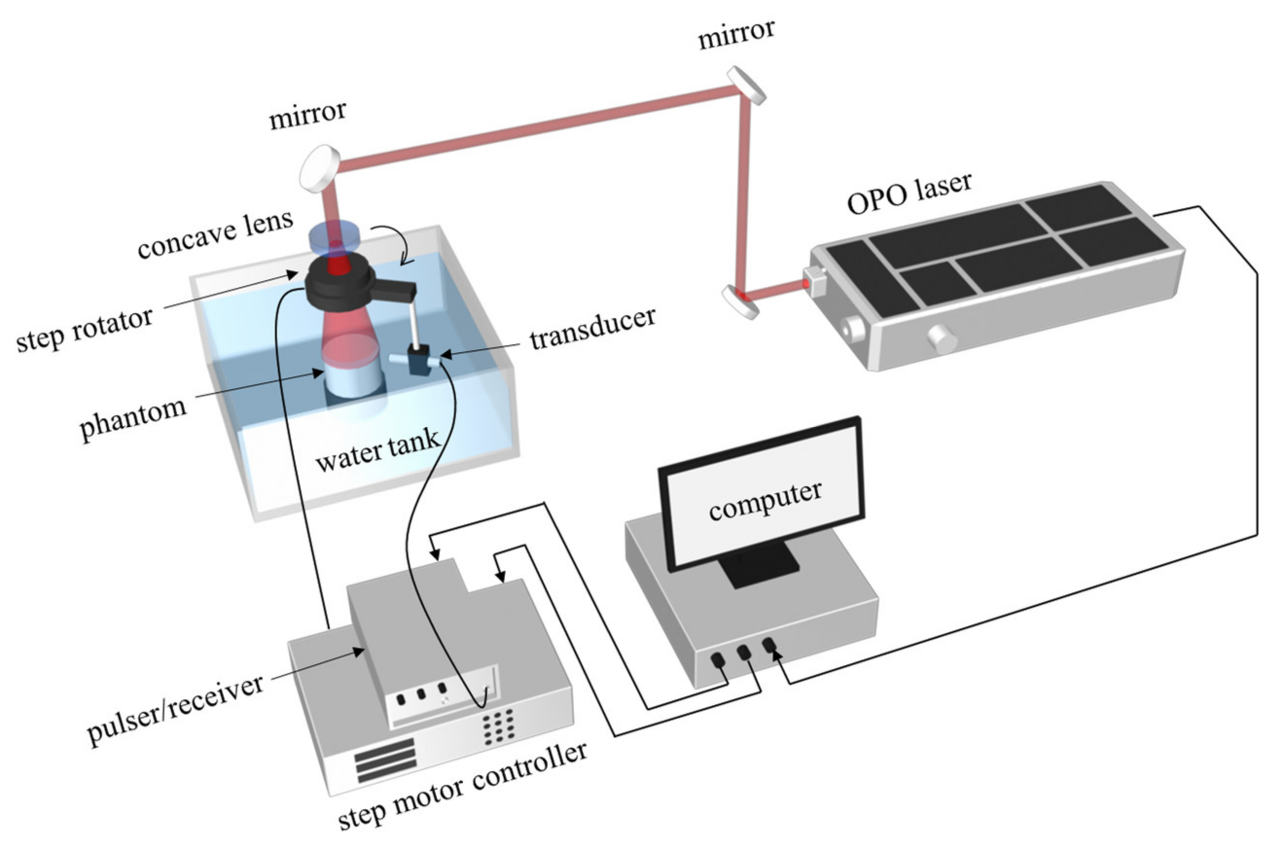
A conventional 2D PAT system was built to test our method, whose schematic is shown in
Figure 3. Pulsed 740 nm laser from an optical parametric oscillator (OPO) laser (SpitLight 600 OPO-532 midband, Innolas, München, Germany) was directed to give illumination of the target. The optical intensity on the top of the phantom was about 5 mJ/cm
2, and the repetition rate was 20 Hz. The total step number of the 2D scan was 360, with an angular step 1 degree. The employed planar transducer (Zunen Industries, Shanghai, China) had a central frequency of 5 MHz, its bandwidth was 80%, and its active element was 3 mm in diameter. The distance between the rotation center to the transducer detection surface was about 20 mm. The signal was first amplified by the a pulser/receiver (DPR500, Ultrasonics California, San Juan Capistrano, CA, USA), and then digitized with an acquisition card (NI-5124, 12 bit, 100 MHz sampling frequency) in the computer. The whole system was synchronized by the laser, and the data were collected on the hard disk for later processing.
Two phantoms were imaged. The phantoms were made of 2% ager, water and intralipid, which had a diameter of 3 cm and a scattering coefficient of 1 /mm. The first phantom had 7 pencil leads (0.5 mm thick) vertically inserted as point targets, and the second phantom had a piece of leaf vein (about 8 mm in size) embedded on its surface.
3. Results
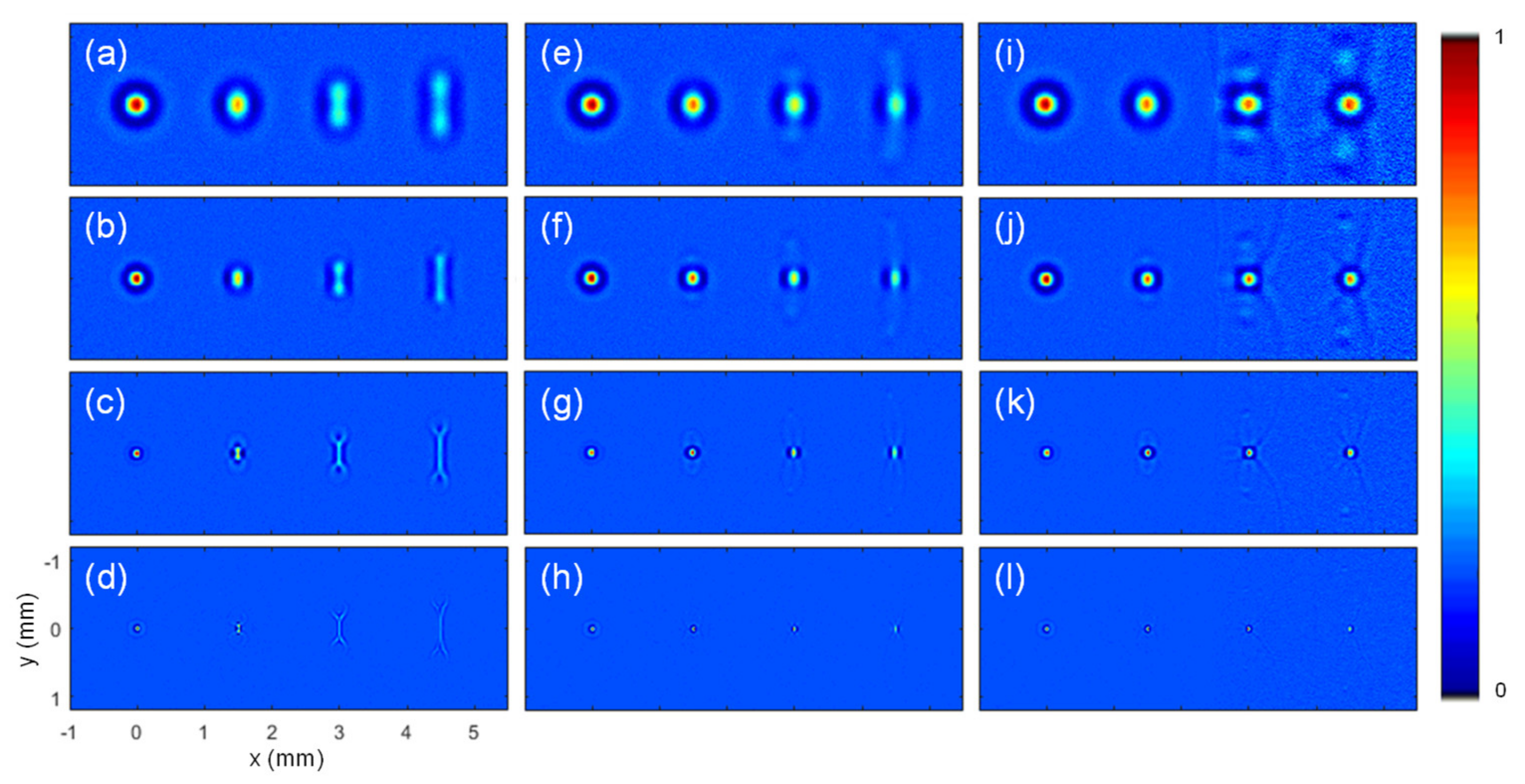
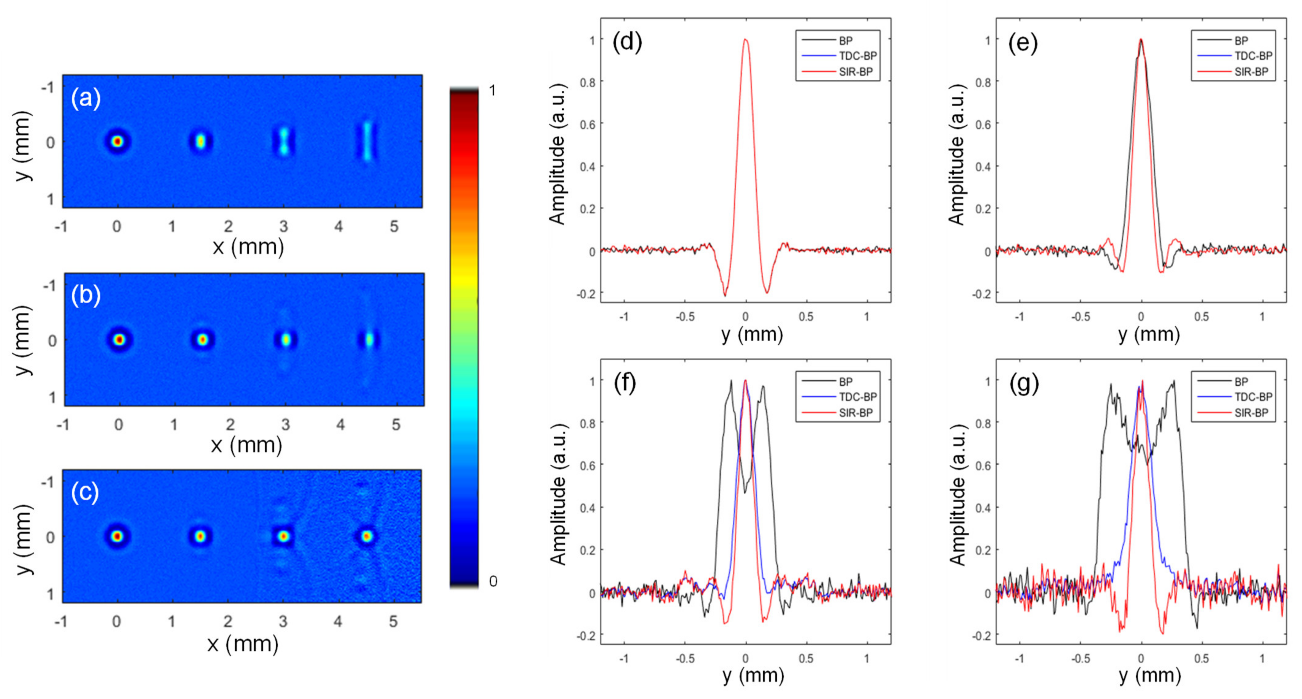
Figure 4 presents the reconstruction results of the simulated data with 5 MHz central frequency and 5 % noise. There were four point-targets evenly distributed on the x-axis from 0 to 4.5 mm. The image domain was −1 mm < x < 5.5 mm, −1.2 mm < y < 1.2 mm. Here,
Figure 4a–c are reconstructed with the conventional BP method (with (3)), the TDC-BP method (with (6)), and the SIR-BP method (with (7)), respectively. Because the transducers were distributed uniformly, the weighting factor
in (3) was set to be one for all the detectors. The cross sections of the four targets in
Figure 4a–c were also extracted and compared in
Figure 4d–g. The full width at half height (FWHM) for all these lateral profiles of the point targets are obtained as lateral resolutions, which are listed in
Table 1 along with the SNRs of the four targets.
It can be seen from
Figure 4 that when the target is away from the center of rotation, the lateral profile of the target becomes wider. For the point target at x = 4.5 mm, it’s lateral resolution was 0.654mm, which was about five times the target of the rotation center (0.136 mm). For the point target at x = 4.5 mm, the lateral resolutions given by the TDC-BP method and the SIR-BP method were 0.204 mm and 0.138 mm, which were about 3.2 and 4.7 times smaller than that given by the conventional BP method.
For SNR comparison and noise assessment, it’s noted that in
Figure 4a,b the background noise is evenly distributed in the image domain. However, the background noise in
Figure 4c is stronger for regions far from the rotation center than the regions near the rotation center. From
Table 1, for all the three off-center targets, both the TDC-BP method and the SIR-BP method give higher SNRs than the conventional BP method. For the target at x = 4.5 mm, the SNR with the conventional BP method is 24.863 dB, but with the TDC-BP method and the SIR-BP method, the SNR improves to 33.311 dB and 27.562 dB, respectively. However, it’s noted that the SNR given by the SIR-BP method is lower than that by the TDC-BP method in the off-center regions. This is due to the fact that the transducer’s sensitivity in the off-center regions is low, so that the background noise in these regions is increased when inverting the SIR amplitude to obtain the weighting factor with (8).
Figure 5 shows the reconstruction results for different central frequencies, as to further explore the adaptability of the proposed method. Here, different rows represent results with different central frequencies, and different columns are reconstructed with different methods.
Table 2 lists the SNRs and FWHMs for the most right-side target at x = 4.5 mm. From the first column, it’s clearly noted that the effect of finite transducer aperture is frequency dependent. For lower frequencies such as 3 MHz and 5 MHz, due to the larger divergence angle of the transducer, the lateral blur is not serious for the target at x = 1.5 mm, which however is more notable for higher frequencies. With the time delay compensation by the TDC-BP method, the lateral blur for the off-center targets is well restored for all the frequencies, and the reconstructed amplitudes of these targets are also increased, which is reflected in the improved SNRs, as in
Table 2. With the SIR-BP method, the lateral resolutions and the reconstructed amplitudes of the off-center targets are also further increased. However, due to the concurrent increased background noise, the SNRs are not as good as those given by the TDC-BP method, but are still better than those by the conventional BP method. As seen in
Table 2, for the target at x = 4.5 mm, the SIR-BP method improves the lateral resolution four to nine times, along with a 3 to 7 dB improvement in the SNR, as compared with the conventional BP method.
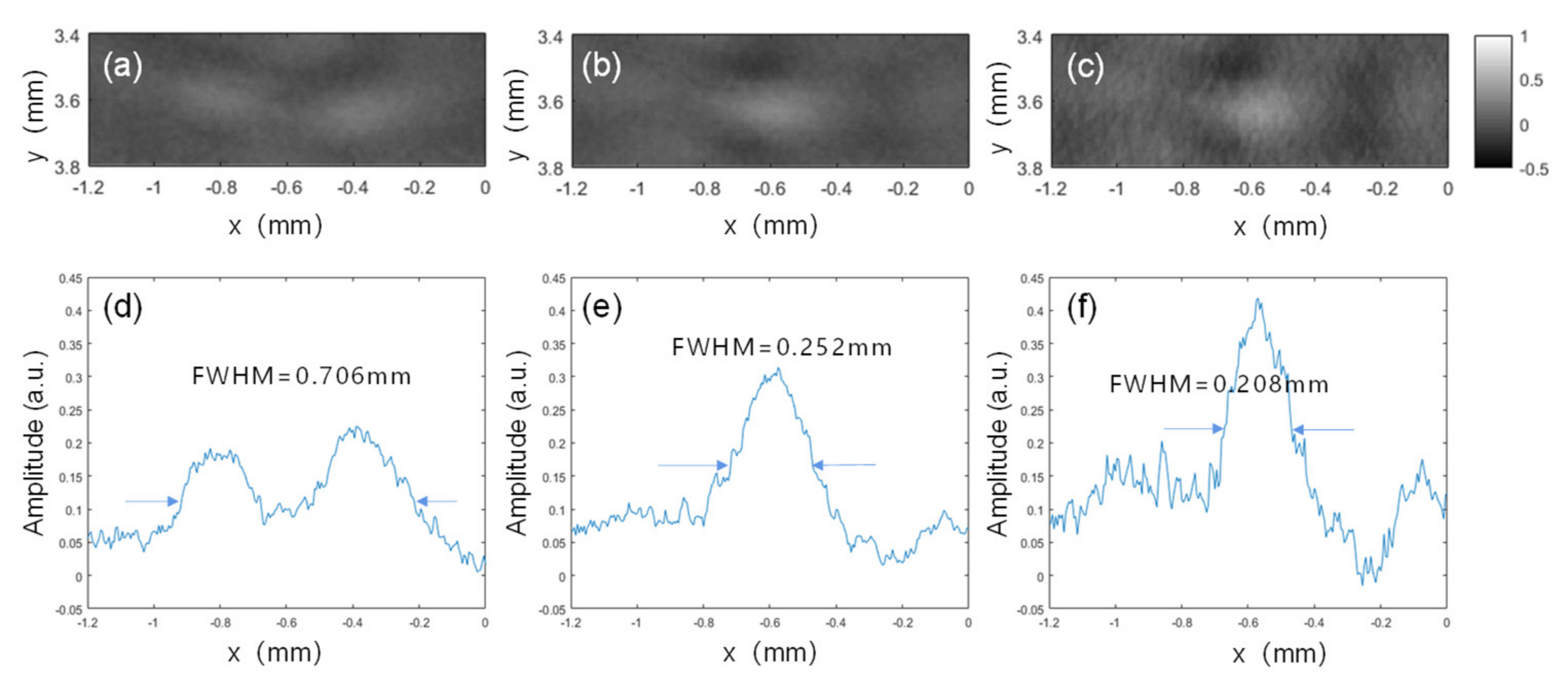
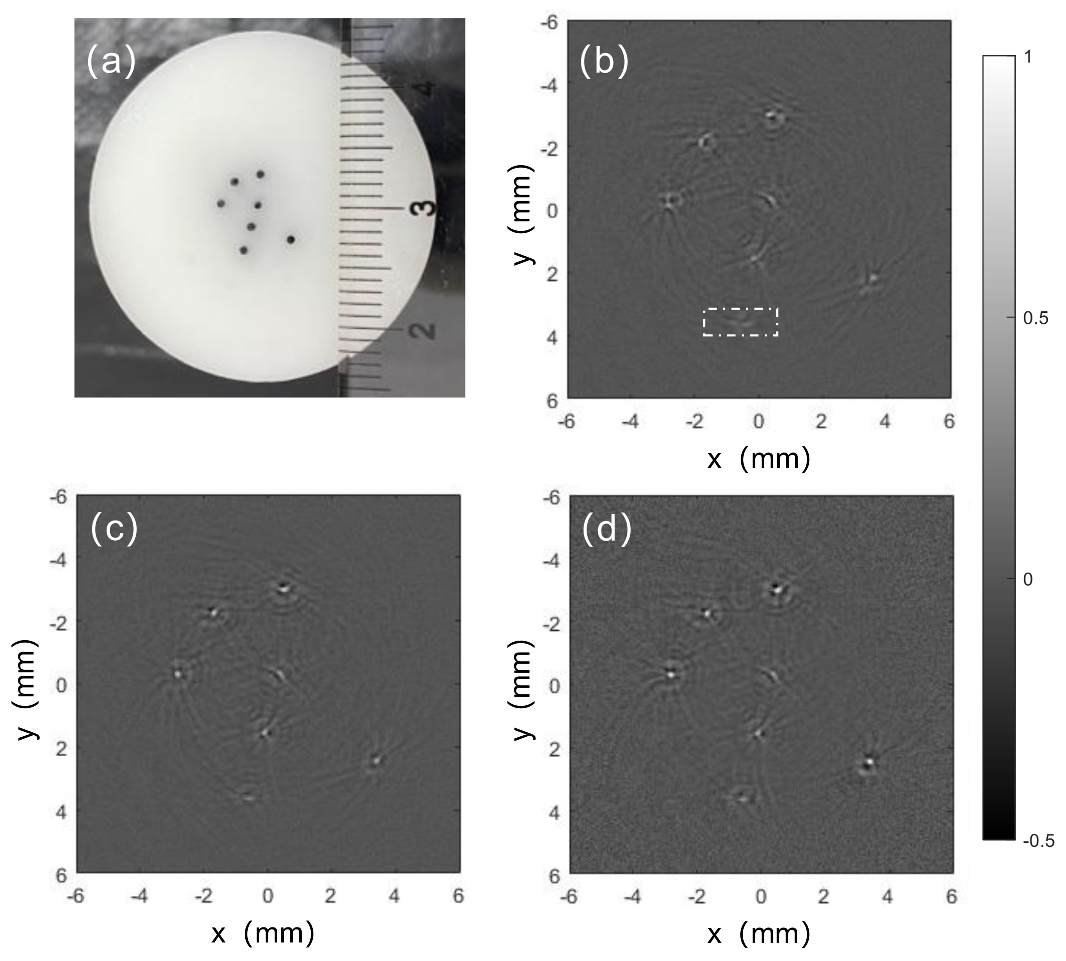
The first phantom experiment was to test the improvement of lateral resolution with our proposed method. There were seven pencil leads vertically inserted in the phantom as point targets, as seen in
Figure 6a, and the reconstructed images with the conventional BP method, the TDC-BP method, and the SIR-BP method are shown in
Figure 6b–d, respectively. Compared with the photo image, it’s seen that all three images can reliably reveal the locations of the seven targets. However, in
Figure 6b the five targets located far from the rotation center are distorted in the lateral directions due to the effect of the finite transducer aperture. With the time delay compensation, the lateral resolutions of these targets are well restored, as seen in
Figure 6c. When directional sensitivity compensation is applied, the lateral blur of these five targets is further reduced in
Figure 6d.
Comparing the obtained FWHMs from the three curves of about 0.70 mm, 0.25 mm and 0.21 mm, it can be seen that the improvement of the FWHM with the TDC-BP and SIR-BP methods were about 2.8 times and 3.3 times, respectively, with respect to the conventional BP method. It’s also noted that the SNRs for
Figure 7d–f were 19.09 dB, 22.78 dB and 19.23 dB, respectively. These results are in good agreement with the conclusions we achieved in the simulation studies.
As seen in
Table 3, in simulation results for the target at x = 4.5 mm, the SIR-BP method improves the lateral resolution four to nine times as compared with the conventional BP method. In phantom experiment result for the target at about 4 mm away from the rotation center, the SIR-BP method improves the lateral resolution 3.3 times as compared with the conventional BP method.
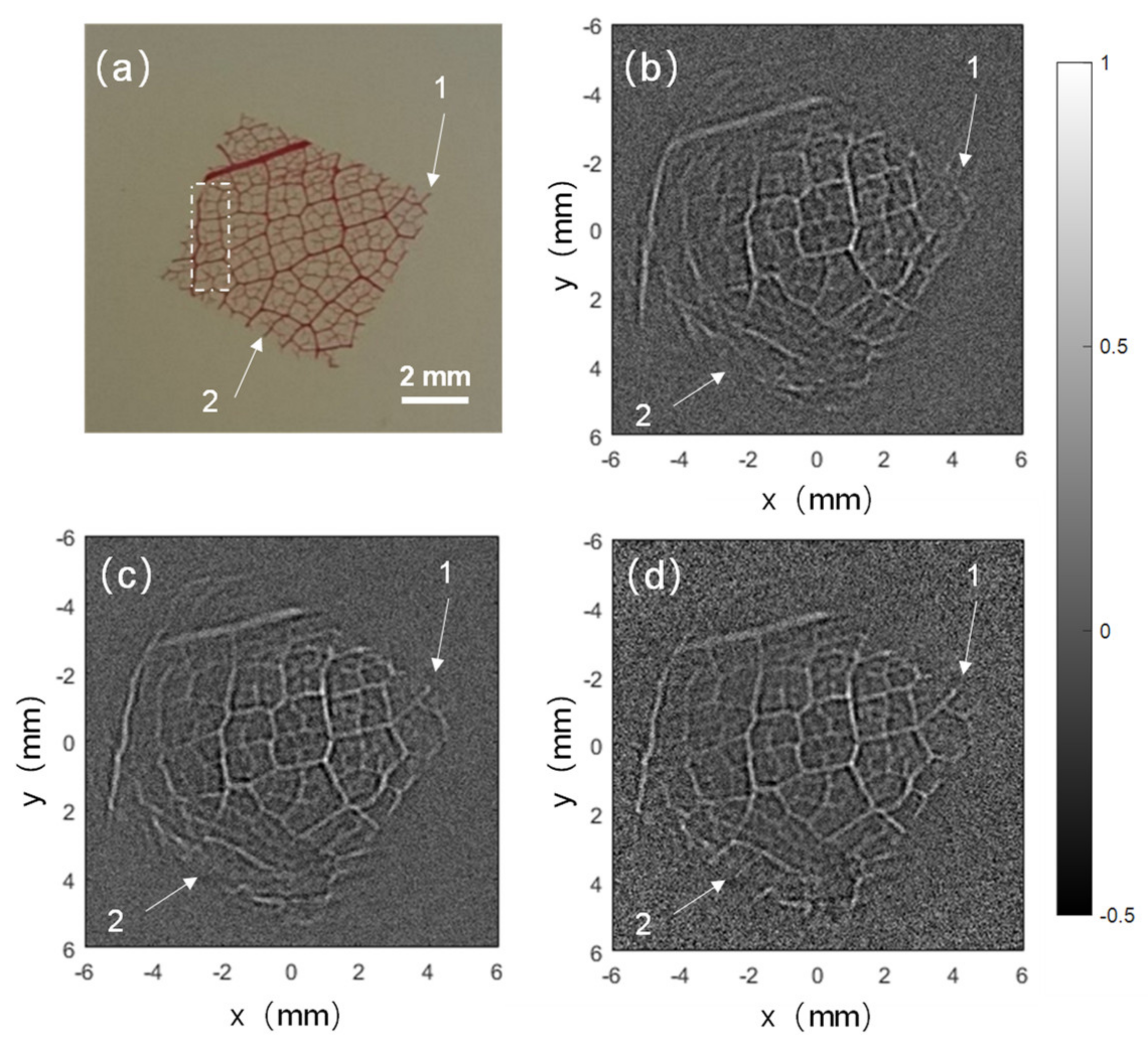
From
Figure 8 we can see the complex reconstruction imaging results of a piece of leaf veins. The size of the leaf veins was about 8 mm. It is noticed that many small structures around the margins of the target were seriously distorted and missed in
Figure 8b. One example is the small branch as indicated with arrow 1. After applying the time delay obtained from the SIR of the transducer, it can be well reconstructed, as seen in
Figure 8c,d. Furthermore, it can be seen that many veins along the axial direction in the dotted rectangle in
Figure 8a were missed in
Figure 8b,c, whereas it can be better revealed in
Figure 8d with the SIR-BP method. Another example is the small branch pointed with arrow 2, which is less clear in
Figure 8c than that in
Figure 8d. This proves the advantage of the SIR-BP method in reconstructing complex objects over the conventional BP method and the TDC-BP method. In
Figure 8d, there is more background noise, and this was because we were trying to suppress the contributions from the in-axial signals while boosting the contributions from the off-axial signals, which makes the signal amplitude low and noise level higher.
In terms of the computational time, because the three methods shared the same BP structure, the reconstruction time cost was similar. For the reconstruction of
Figure 8, which had 601 × 601 pixels and 360 detectors, the time cost with the conventional BP method, the TDC-BP method and the SIR-BP method were 15.2 s, 18.3 s, and 20.2 s, respectively, running on a single CPU (1.80 GHz) on MATLAB.
4. Discussion
The “finite aperture effect” is one of the biggest problem that hinders the acquisition of high-quality images in circular/spherical-scanning-based PACT. The purpose of this paper is to find a fast and stable image reconstruction method for tackling this problem. Because the degraded lateral resolution is largely due to the time delay error and spatial-dependent sensitivity introduced by the SIR of the finite transducer aperture, this work proposes to calculate and compensate for these two factors in the framework of the BP method. Therefore, compared with existing model-based algorithms [
18,
27,
28,
29] for this “finite aperture effect” problem, our proposed method inherits the simplicity, stability and low computation cost from the BP method [
30,
31], so that it is more practical.
The proposed method was validated with both numerical simulations and phantom experiments. As seen in the simulation study, by correcting the time delay in the BP equation with the SIR, both the lateral resolution and SNR in the off-center regions are effectively improved. By further compensating the sensitivity loss in the off-center regions with the SIR-BP method, simulation results indicate that the elongated lateral resolution can almost be completely restored.
It is noted that our proposed method was tested in simulations in the frequency range from 3 MHz to 20 MHz, which covers the common frequency range of existing PAT systems. Results showed that the proposed method showed consistent improvement of the lateral resolution and the SNRs over the conventional BP method, which proves its adaptability and effectiveness. The stability of the proposed method has also been proved with simulated data with 5% noise and the experimental data. In addition, the SIR-BP method is almost as fast as the conventional BP method and the TDC-BP method in terms of run time. All these indicates that the SIR-BP method is a better alternative to the conventional BP method, and can be used for guidance of system designs.
The proposed method has been successfully tested with two phantom experiments. The first experiment validated the improvement in lateral resolution and SNR with the proposed method. The second experiment was to explore the potential of the proposed method for imaging complicated targets. Results showed the proposed method can well recover the blurred structures in the off-center regions, especially for small features along the axial directions. In short, the proposed SIR-BP method can comprehensively improve the image fidelity. In future works, we will accelerate the proposed method with GPU based parallel techniques [
32], and extend it to the spherical-scanning-based PAT for 3D imaging.


