Electromagnetic Hanbury Brown and Twiss Effect in Atmospheric Turbulence

Abstract

The evolution of the 4 × 4 matrix with elements being the scintillation indices of the single-point Stokes parameters of a stationary electromagnetic beam-like optical field in classic, weak atmospheric turbulence is revealed. It is shown that depending on the choice of the source parameters, the source-induced changes in the matrix elements of the propagating beam and those produced by turbulence can be either range-separated or conjoined. For theoretical analysis, the unified theory of coherence and polarization is used together with the extended Huygens-Fresnel integral approach. The results can be of interest for building robust communication and sensing systems operating in the presence of atmospheric fluctuations.

1. Introduction

The discovery by Hanbury Brown and Twiss of non-trivial correlations in the intensity of spatially separated, fluctuating, classic light fields [1,2] has led to a number of ground-breaking technologies, the most important of which are the stellar interferometry [3] and ghost imaging [4]. In the majority of scenarios, the measured light field is thermal, i.e., obeys the circular Gaussian statistics, and, hence, involves a very simple relation between the field correlations and the intensity correlations, as a consequence of the Gaussian moment theorem [5].

Another area greatly benefiting from the optical intensity correlation analysis is the laser beam interaction with atmospheric turbulence, including a variety of applications, such as remote sensing, classic imaging, and free-space optical communications [6]. The laser beams, initially fully spatially coherent, are modulated by the air’s fluctuating refractive index, being a very complex and non-Gaussian random process. The intensity correlations of the laser field interacting with turbulence hence carry a complex signature of the atmospheric refractive index’s random process, which cannot be directly related to that acquired by field correlations.

Light fields radiated by thermal and partially coherent sources have also been studied on interaction with atmospheric turbulence, mostly under scalar treatment [7,8,9,10,11,12]. In such situations, the fluctuations in the optical field propagating through turbulence are also governed by a random process different from Gaussian. The usefulness of the spatially pre-randomized optical fields, however, is in the reduction of their intensity fluctuations as compared with those in a beam with the same geometry launched into the same turbulence channel by a laser. This idea was employed a number of times for improving the quality of free-space optical communications [13,14,15].

The original Hanbury Brown and Twiss experiment was based on the unpolarized, thermal light and relied on the scalar coherence theory. However, partially coherent light sources were later introduced that can have arbitrary polarization distribution and arbitrary vectorial spatial correlations [16,17]. Such sources can exhibit changes in coherence and polarization states as the generated field evolves, even in free space. Furthermore, for such sources, the vectorial version of the Brown and Twiss correlations was studied for the instantaneous intensity and the instantaneous single-point Stokes vector [18,19,20]. Free-space evolution and weak scattering of self-correlations in the single-point Stokes parameters of such fields were examined, under the Gaussian statistics assumption [21,22]. Also, the atmospheric propagation of the single-point Stokes parameters’ self-correlations (but not the joint correlations) was studied in theory, via computer simulations and experiments [23,24,25,26].

The most general Hanbury Brown and Twiss 4 × 4 correlation matrix of the optical vector field having the diagonal/off-diagonal elements occupied with the self-correlations/joint correlations of the instantaneous Stokes parameters was recently introduced in [27], and its free-space evolution and interaction with optical systems were examined in [28]. A related study elucidating the behavior of the degree of cross-polarization (a quantity derived from the electromagnetic intensity–intensity correlations) in the classic atmospheric turbulence was also performed [29,30]. This study, however, was entirely based on the second-order coherence theory.

The purpose of this paper is to investigate the behavior of the 4 × 4 Hanbury Brown and Twiss correlation matrix in the atmospheric turbulence depending on the source and turbulence parameters. The taken approach relies on the Extended Huygens Fresnel (EHF) integral developed for the second and the fourth-order electromagnetic field correlations [6] (see also [31] for discussion about the limitations of the EHF integral).

The practical use of our work is anticipated in free-space communications in which 16 polarization-based sub-channels can be established by a single optical source. The quality of each channel can be controlled by modulating the individual elements of the 4 × 4 Hanbury Brown and Twiss matrix at the source plane.

2. Method

2.1. The Average Stokes Parameters in Turbulence

The cross-spectral density matrix of an electromagnetic beam at positions ${\mathbf{r}}_1$ and ${\mathbf{r}}_2$ (where ${\mathbf{r}}_1=({\mathit{\rho }}_1,z)$ and ${\mathbf{r}}_2=({\mathit{\rho }}_2,z)$, ${\mathit{\rho }}_1$ and ${\mathit{\rho }}_2$ are two-dimensional transverse position vectors, z is the direction of propagation) and at frequency $\omega$ is given as [16]:

$$\mathbf{W}({\mathbf{r}}_1,{\mathbf{r}}_2,\omega )=\left(\begin{array}{cc}{W}_{xx}& W_{xy}\\ W_{yx}& W_{yy}\end{array}\right),$$

(1)

where the matrix elements are

$$W_{\alpha \beta }({\mathbf{r}}_1,{\mathbf{r}}_2,\omega )=\langle E_{\alpha }^{\ast }({\mathbf{r}}_1,\omega )E_{\beta }({\mathbf{r}}_2,\omega )\rangle \hspace{0.17em}\hspace{0.17em}\hspace{0.17em}\hspace{0.17em}\hspace{0.17em}\hspace{0.17em}\hspace{0.17em}\hspace{0.17em}\hspace{0.17em}(\alpha ,\beta =x,y),$$

(2)

with $E_{\alpha }(\mathbf{r},\omega )$ being a realization of the Cartesian component $\alpha$ of the beam-like electric field. Here $\ast$ and $\langle .\rangle$ denote the complex conjugation and the average over the ensemble of monochromatic realizations, respectively. The single-point Stokes parameters are related to the cross-spectral density matrix elements as follows [17]:

$$\langle S_0(\mathbf{r},\omega )\rangle =W_{xx}(\mathbf{r},\mathbf{r},\omega )+W_{yy}(\mathbf{r},\mathbf{r},\omega ),$$

(3a)

$$\langle S_1(\mathbf{r},\omega )\rangle =W_{xx}(\mathbf{r},\mathbf{r},\omega )-W_{yy}(\mathbf{r},\mathbf{r},\omega ),$$

(3b)

$$\langle S_2(\mathbf{r},\omega )\rangle =W_{xy}(\mathbf{r},\mathbf{r},\omega )+W_{yx}(\mathbf{r},\mathbf{r},\omega ),$$

(3c)

$$\langle S_3(\mathbf{r},\omega )\rangle =i\left[W_{yx}(\mathbf{r},\mathbf{r},\omega )-W_{xy}(\mathbf{r},\mathbf{r},\omega )\right],$$

(3d)

where the angular brackets are used here in contrast with a classic notation to distinguish the averaged and the instantaneous sets of parameters (the latter will be introduced below). Further, the two-point (generalized) Stokes parameters are defined as [32].

$$\langle S_0({\mathbf{r}}_1,{\mathbf{r}}_2,\omega )\rangle =W_{xx}({\mathbf{r}}_1,{\mathbf{r}}_2,\omega )+W_{yy}({\mathbf{r}}_1,{\mathbf{r}}_2,\omega ),$$

(4a)

$$\langle S_1({\mathbf{r}}_1,{\mathbf{r}}_2,\omega )\rangle =W_{xx}({\mathbf{r}}_1,{\mathbf{r}}_2,\omega )-W_{yy}({\mathbf{r}}_1,{\mathbf{r}}_2,\omega ),$$

(4b)

$$\langle S_2({\mathbf{r}}_1,{\mathbf{r}}_2,\omega )\rangle =W_{xy}({\mathbf{r}}_1,{\mathbf{r}}_2,\omega )+W_{yx}({\mathbf{r}}_1,{\mathbf{r}}_2,\omega ),$$

(4c)

$$\langle S_3({\mathbf{r}}_1,{\mathbf{r}}_2,\omega )\rangle =i\left[W_{yx}({\mathbf{r}}_1,{\mathbf{r}}_2,\omega )-W_{xy}({\mathbf{r}}_1,{\mathbf{r}}_2,\omega )\right].$$

(4d)

On assuming that a beam propagates in free space from the source plane $z=0$ into half-space $z>0$, close to the positive z-direction, and that the realizations of the electric field components in the source plane and in the receiver plane, at the point is $\mathbf{r}=(\mathit{\rho },z)$, are $E_{\alpha }^s({\mathit{\rho }}^{\prime },\omega )$ and $E_{\alpha }(\mathit{\rho },z,\omega )$ respectively, the relation between them can be expressed via the Huygens-Fresnel integral [17,33]:

$$E_{\alpha }(\mathit{\rho },z,\omega )={\displaystyle \underset{-\infty }{\overset{\infty }{\int }}{E}_{\alpha }^s({\mathit{\rho }}^{\prime },\omega )}G(\mathit{\rho }-{\mathit{\rho }}^{\prime },z,\omega ){\mathrm{d}}^2{\mathit{\rho }}^{\prime },\hspace{0.17em}\hspace{0.17em}\hspace{0.17em}\hspace{0.17em}\hspace{0.17em}\hspace{0.17em}\alpha =x,y,$$

(5)

where $G(\mathit{\rho }-{\mathit{\rho }}^{\prime },z,\omega )$ is the free-space Green’s function of a point source:

$$G(\mathit{\rho }-{\mathit{\rho }}^{\prime },z,\omega )=-\frac{ik}{2\pi z}\exp \left[\frac{ik{\left(\mathit{\rho }-{\mathit{\rho }}^{\prime }\right)}^2}{2z}\right],$$

(6)

with $k=\omega /c$ and $c$ being the speed of light in a vacuum. Then the elements of the cross-spectral density matrices at a pair of points in the source plane and in the receiver plane are related as:

$$\begin{array}{l}{W}_{\alpha \beta }({\mathbf{r}}_1,{\mathbf{r}}_2,\omega )={\displaystyle \underset{-\infty }{\overset{\infty }{\int }}{\displaystyle \underset{-\infty }{\overset{\infty }{\int }}{\mathrm{d}}^2{\mathit{\rho }}_1{}^{\prime }{\mathrm{d}}^2{\mathit{\rho }}_2{}^{\prime }{W}_{\alpha \beta }({\mathit{\rho }}_1{}^{\prime },{\mathit{\rho }}_2{}^{\prime },z=0)}}\\ \hspace{0.17em}\hspace{0.17em}\hspace{0.17em}\hspace{0.17em}\hspace{0.17em}\hspace{0.17em}\hspace{0.17em}\hspace{0.17em}\hspace{0.17em}\hspace{0.17em}\hspace{0.17em}\hspace{0.17em}\hspace{0.17em}\hspace{0.17em}\hspace{0.17em}\hspace{0.17em}\hspace{0.17em}\hspace{0.17em}\times G^{\ast }({\mathit{\rho }}_1-{\mathit{\rho }}_1{}^{\prime },z,\omega )G({\mathit{\rho }}_2-{\mathit{\rho }}_2{}^{\prime },z,\omega ),\hspace{0.17em}\hspace{0.17em}\hspace{0.17em}\hspace{0.17em}\hspace{0.17em}\hspace{0.17em}\hspace{0.17em}\hspace{0.17em}\hspace{0.17em}\alpha =x,y,\hspace{0.17em}\hspace{0.17em}\hspace{0.17em}\hspace{0.17em}\beta =x,y.\end{array}$$

(7)

If the half-space z > 0 is filled with classic (homogeneous, isotropic, Kolmogorov-like) atmospheric turbulence, the product of the Green’s functions become its second-order correlation function [6]:

$$\begin{array}{l}\langle G^{\ast }({\mathit{\rho }}_1-{\mathit{\rho }}_1{}^{\prime },z,\omega )G({\mathit{\rho }}_2-{\mathit{\rho }}_2{}^{\prime },z,\omega )\rangle \\ \hspace{0.17em}\hspace{0.17em}\hspace{0.17em}\hspace{0.17em}\hspace{0.17em}\hspace{0.17em}\hspace{0.17em}\hspace{0.17em}\hspace{0.17em}\hspace{0.17em}\hspace{0.17em}\hspace{0.17em}\hspace{0.17em}\hspace{0.17em}={\left(\frac{k}{2\pi z}\right)}^2\exp \left\{-\frac{ik}{2z}\left[{\left({\mathit{\rho }}_1-{\mathit{\rho }}_1{}^{\prime }\right)}^2-{\left({\mathit{\rho }}_2-{\mathit{\rho }}_2{}^{\prime }\right)}^2\right]\right\}\\ \hspace{0.17em}\hspace{0.17em}\hspace{0.17em}\hspace{0.17em}\hspace{0.17em}\hspace{0.17em}\hspace{0.17em}\hspace{0.17em}\hspace{0.17em}\hspace{0.17em}\hspace{0.17em}\hspace{0.17em}\hspace{0.17em}\hspace{0.17em}\times \exp \{-\frac{{\pi }^2{k}^{2}z}{3}{\displaystyle \underset{0}{\overset{\infty }{\int }}{\kappa }^3{\mathsf{\Phi }}_n(\kappa )d\kappa }\left[{\left({\mathit{\rho }}_1-{\mathit{\rho }}_2\right)}^2+\left({\mathit{\rho }}_1-{\mathit{\rho }}_2\right)\left({\mathit{\rho }}_1{}^{\prime }-{\mathit{\rho }}_2{}^{\prime }\right)+{\left({\mathit{\rho }}_1{}^{\prime }-{\mathit{\rho }}_2{}^{\prime }\right)}^2\right]\}\end{array}$$

(8)

where ${\mathsf{\Phi }}_n(\kappa )$ is the turbulence power spectrum and $\kappa$ is the spatial frequency. This implies that the cross-spectral density matrix elements become:

$$\begin{array}{l}{W}_{\alpha \beta }({\mathbf{r}}_1,{\mathbf{r}}_2,\omega )={\left(\frac{k}{2\pi z}\right)}^2{\displaystyle \underset{-\infty }{\overset{\infty }{\int }}{\displaystyle \underset{-\infty }{\overset{\infty }{\int }}{\mathrm{d}}^2{\mathit{\rho }}_1{}^{\prime }{\mathrm{d}}^2{\mathit{\rho }}_2{}^{\prime }{W}_{\alpha \beta }({\mathit{\rho }}_1{}^{\prime },{\mathit{\rho }}_2{}^{\prime },z=0)}}\exp \left\{-\frac{ik}{2z}\left[{\left({\mathit{\rho }}_1-{\mathit{\rho }}_1{}^{\prime }\right)}^2-{\left({\mathit{\rho }}_2-{\mathit{\rho }}_2{}^{\prime }\right)}^2\right]\right\}\\ \hspace{0.17em}\hspace{0.17em}\hspace{0.17em}\hspace{0.17em}\hspace{0.17em}\hspace{0.17em}\hspace{0.17em}\hspace{0.17em}\hspace{0.17em}\hspace{0.17em}\hspace{0.17em}\hspace{0.17em}\hspace{0.17em}\hspace{0.17em}\hspace{0.17em}\hspace{0.17em}\hspace{0.17em}\hspace{0.17em}\hspace{0.17em}\hspace{0.17em}\hspace{0.17em}\hspace{0.17em}\times \exp \{-\frac{{\pi }^2{k}^{2}z}{3}{\displaystyle \underset{0}{\overset{\infty }{\int }}{\kappa }^3{\mathsf{\Phi }}_n(\kappa )d\kappa }\left[{\left({\mathit{\rho }}_1-{\mathit{\rho }}_2\right)}^2+\left({\mathit{\rho }}_1-{\mathit{\rho }}_2\right)\left({\mathit{\rho }}_1{}^{\prime }-{\mathit{\rho }}_2{}^{\prime }\right)+{\left({\mathit{\rho }}_1{}^{\prime }-{\mathit{\rho }}_2{}^{\prime }\right)}^2\right]\}.\end{array}$$

(9)

If the source radiating the beam is of the electromagnetic Gaussian Schell model class, its cross-spectral density matrix has the form [17]:

$$W_{\alpha \beta }({\mathbf{r}}_1,{\mathbf{r}}_2,z=0)=A_{\alpha }{A}_{\beta }{B}_{\alpha \beta }\exp \left[-\frac{1}{4{\sigma }^2}\left({{\mathit{\rho }}^{\prime }}_1^2+{{\mathit{\rho }}^{\prime }}_2^2\right)\right]\exp \left[-\frac{1}{2{\delta }_{\alpha \beta }^2}{\left({\mathit{\rho }}_1{}^{\prime }-{\mathit{\rho }}_2{}^{\prime }\right)}^2\right],\hspace{0.17em}\hspace{0.17em}\hspace{0.17em}\hspace{0.17em}\hspace{0.17em}\hspace{0.17em}\hspace{0.17em}\hspace{0.17em}\alpha ,\beta =x,y.$$

(10)

Here $A_{\alpha }$ and $A_{\beta }$ are the amplitudes of the electric field vector components $E_{\alpha }$ and $E_{\beta }$, $B_{\alpha \beta }$ is the correlation coefficient between $E_{\alpha }$ and $E_{\beta }$ components, $B_{xy}=B_{xy}\exp \left(-j\varphi \right)$, $\varphi$ is the phase of the xy component, $B_{xy}=B_{yx}^{\ast }$, ${\sigma }^2$ is the variance of the source spectral density width and ${\delta }_{\alpha \beta }^2$ is the variance of the correlation between components $E_{\alpha }$ and $E_{\beta }$. The parameters of the source must satisfy the beam conditions and the realizability conditions that are the consequence of the non-negative definiteness and quasi-Hermiticity of the cross-spectral density matrix [17]. Substituting from Equation (10) into Equation (9) yields:

$$\begin{array}{l}{W}_{\alpha \beta }({\mathbf{r}}_1,{\mathbf{r}}_2,\omega )=A_{\alpha }{A}_{\beta }{B}_{\alpha \beta }{\left(\frac{k}{2\pi z}\right)}^2{\displaystyle \underset{-\infty }{\overset{\infty }{\int }}{\displaystyle \underset{-\infty }{\overset{\infty }{\int }}{\mathrm{d}}^2{\mathit{\rho }}_1{}^{\prime }{\mathrm{d}}^2{\mathit{\rho }}_2{}^{\prime }\exp \left[-\frac{1}{4{\sigma }^2}\left({{\mathit{\rho }}^{\prime }}_1^2+{{\mathit{\rho }}^{\prime }}_2^2\right)\right]}}\exp \left[-\frac{1}{2{\delta }_{\alpha \beta }^2}{\left({\mathit{\rho }}_1{}^{\prime }-{\mathit{\rho }}_2{}^{\prime }\right)}^2\right]\\ \hspace{0.17em}\hspace{0.17em}\hspace{0.17em}\hspace{0.17em}\hspace{0.17em}\hspace{0.17em}\hspace{0.17em}\hspace{0.17em}\hspace{0.17em}\hspace{0.17em}\hspace{0.17em}\hspace{0.17em}\hspace{0.17em}\hspace{0.17em}\hspace{0.17em}\hspace{0.17em}\hspace{0.17em}\hspace{0.17em}\hspace{0.17em}\hspace{0.17em}\hspace{0.17em}\hspace{0.17em}\times \exp \left\{-\frac{ik}{2z}\left[{\left({\mathit{\rho }}_1-{\mathit{\rho }}_1{}^{\prime }\right)}^2-{\left({\mathit{\rho }}_2-{\mathit{\rho }}_2{}^{\prime }\right)}^2\right]\right\}\exp \{-\frac{{\pi }^2{k}^{2}z}{3}{\displaystyle \underset{0}{\overset{\infty }{\int }}{\kappa }^3{\mathsf{\Phi }}_n(\kappa )d\kappa }\\ \hspace{0.17em}\hspace{0.17em}\hspace{0.17em}\hspace{0.17em}\hspace{0.17em}\hspace{0.17em}\hspace{0.17em}\hspace{0.17em}\hspace{0.17em}\hspace{0.17em}\hspace{0.17em}\hspace{0.17em}\hspace{0.17em}\hspace{0.17em}\hspace{0.17em}\hspace{0.17em}\hspace{0.17em}\hspace{0.17em}\hspace{0.17em}\hspace{0.17em}\hspace{0.17em}\hspace{0.17em}\times \left[{\left({\mathit{\rho }}_1-{\mathit{\rho }}_2\right)}^2+\left({\mathit{\rho }}_1-{\mathit{\rho }}_2\right)\left({\mathit{\rho }}_1{}^{\prime }-{\mathit{\rho }}_2{}^{\prime }\right)+{\left({\mathit{\rho }}_1{}^{\prime }-{\mathit{\rho }}_2{}^{\prime }\right)}^2\right]\}.\end{array}$$

(11)

Using Tatarskii’s power spectrum ${\mathsf{\Phi }}_n(\kappa )=0.033C_n^2{\kappa }^{-11/3}\exp \left(-{\kappa }^2/{\kappa }_m^2\right)$ where $C_n^2$ is the refractive-index structure constant, ${\kappa }_m=5.92/l_0$, $l_0$ is the Kolmogorov inner scale length [34], one finds that $P=\frac{{\pi }^2{k}^{2}z}{3}{\displaystyle \underset{0}{\overset{\infty }{\int }}{\kappa }^3{\mathsf{\Phi }}_n(\kappa )d\kappa }=0.55C_n^2{l}_0^{-1/3}{k}^{2}z$, and hence,

$$\begin{array}{l}{W}_{\alpha \beta }({\mathbf{r}}_1,{\mathbf{r}}_2,\omega )=A_{\alpha }{A}_{\beta }{B}_{\alpha \beta }{\left(\frac{k}{2\pi z}\right)}^2{\displaystyle \underset{-\infty }{\overset{\infty }{\int }}{\displaystyle \underset{-\infty }{\overset{\infty }{\int }}{\mathrm{d}}^2{\mathit{\rho }}_1{}^{\prime }{\mathrm{d}}^2{\mathit{\rho }}_2{}^{\prime }\exp \left[-\frac{1}{4{\sigma }^2}\left({{\mathit{\rho }}^{\prime }}_1^2+{{\mathit{\rho }}^{\prime }}_2^2\right)\right]}}\\ \hspace{0.17em}\hspace{0.17em}\hspace{0.17em}\hspace{0.17em}\hspace{0.17em}\hspace{0.17em}\hspace{0.17em}\hspace{0.17em}\hspace{0.17em}\hspace{0.17em}\hspace{0.17em}\hspace{0.17em}\hspace{0.17em}\hspace{0.17em}\hspace{0.17em}\hspace{0.17em}\hspace{0.17em}\hspace{0.17em}\hspace{0.17em}\times \exp \left[-\frac{1}{2{\delta }_{\alpha \beta }^2}{\left({\mathit{\rho }}_1{}^{\prime }-{\mathit{\rho }}_2{}^{\prime }\right)}^2\right]\exp \left\{-\frac{ik}{2z}\left[{\left({\mathit{\rho }}_1-{\mathit{\rho }}_1{}^{\prime }\right)}^2-{\left({\mathit{\rho }}_2-{\mathit{\rho }}_2{}^{\prime }\right)}^2\right]\right\}\\ \hspace{0.17em}\hspace{0.17em}\hspace{0.17em}\hspace{0.17em}\hspace{0.17em}\hspace{0.17em}\hspace{0.17em}\hspace{0.17em}\hspace{0.17em}\hspace{0.17em}\hspace{0.17em}\hspace{0.17em}\hspace{0.17em}\hspace{0.17em}\hspace{0.17em}\hspace{0.17em}\hspace{0.17em}\hspace{0.17em}\hspace{0.17em}\times \exp \left\{-P\left[{\left({\mathit{\rho }}_1-{\mathit{\rho }}_2\right)}^2+\left({\mathit{\rho }}_1-{\mathit{\rho }}_2\right)\left({\mathit{\rho }}_1{}^{\prime }-{\mathit{\rho }}_2{}^{\prime }\right)+{\left({\mathit{\rho }}_1{}^{\prime }-{\mathit{\rho }}_2{}^{\prime }\right)}^2\right]\right\}.\end{array}$$

(12)

Changing variables as ${{\mathit{\rho }}^{\prime }}_s=\frac{1}{2}\left({\mathit{\rho }}_1{}^{\prime }+{\mathit{\rho }}_2{}^{\prime }\right)$ and ${{\mathit{\rho }}^{\prime }}_d=\left({\mathit{\rho }}_1{}^{\prime }-{\mathit{\rho }}_2{}^{\prime }\right)$, and after performing integrations, Equation (12) reduces to form (see Appendix A):

$$\begin{array}{l}{W}_{\alpha \beta }({\mathbf{r}}_1,{\mathbf{r}}_2,\omega )=A_{\alpha }{A}_{\beta }{B}_{\alpha \beta }\frac{{\sigma }^2}{{\Delta }_1}{\left(\frac{k}{2z}\right)}^2\exp \left(-\frac{ik}{z}{\mathit{\rho }}_s{\mathit{\rho }}_d\right)\exp \left\{-\left[P-{\sigma }^2{\left(\frac{ik}{z}\right)}^2\right]{\mathit{\rho }}_d^2\right\}\\ \hspace{0.17em}\hspace{0.17em}\hspace{0.17em}\hspace{0.17em}\hspace{0.17em}\hspace{0.17em}\hspace{0.17em}\hspace{0.17em}\hspace{0.17em}\hspace{0.17em}\hspace{0.17em}\hspace{0.17em}\hspace{0.17em}\hspace{0.17em}\hspace{0.17em}\hspace{0.17em}\hspace{0.17em}\hspace{0.17em}\hspace{0.17em}\times \exp \left[\frac{1}{2{\Delta }_1}{\left({\Delta }_2{\mathit{\rho }}_d+{\Delta }_3{\mathit{\rho }}_s\right)}^2\right],\end{array}$$

(13)

where ${\mathit{\rho }}_s=\frac{1}{2}\left({\mathit{\rho }}_1+{\mathit{\rho }}_2\right)$, ${\mathit{\rho }}_d=\left({\mathit{\rho }}_1-{\mathit{\rho }}_2\right)$, ${\Delta }_1=\left(\frac{1}{2{\delta }_{\alpha \beta }^2}+\frac{1}{8{\sigma }^2}+P+\frac{{\sigma }^2{k}^2}{z^2}\right)$, ${\Delta }_2=2\frac{{\sigma }^2{k}^2}{z^2}-P$ and ${\Delta }_3=\frac{ik}{z}$.

2.2. The Correlations in Stokes Parameters in Turbulence

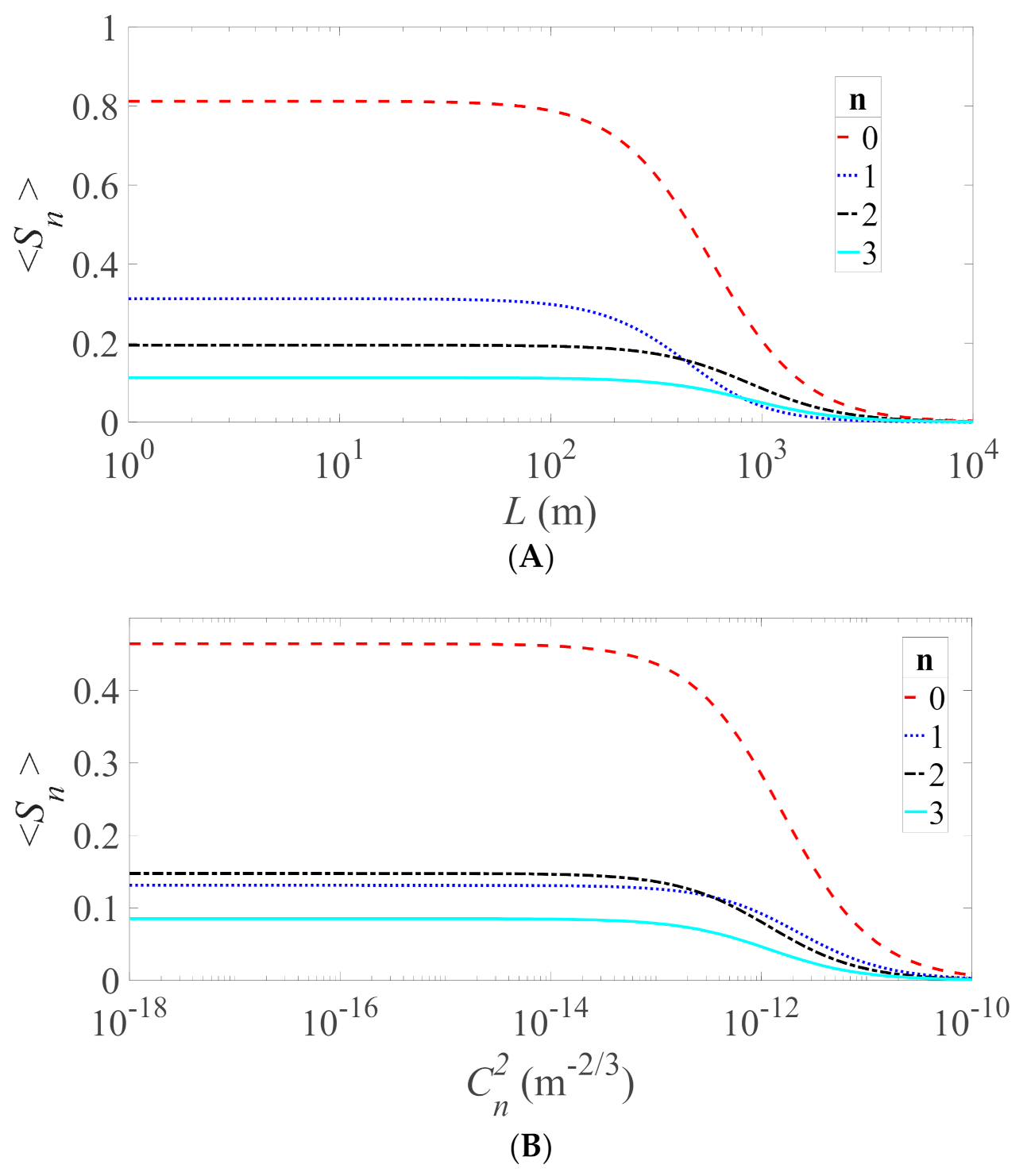
The fluctuation in each instantaneous Stokes parameter about its average value can be defined as:

$$\Delta S_n(\mathbf{r},\omega )=S_n(\mathbf{r},\omega )-\langle S_n(\mathbf{r},\omega )\rangle ,\hspace{0.17em}\hspace{0.17em}\hspace{0.17em}\hspace{0.17em}\hspace{0.17em}\hspace{0.17em}n=0,1,2,3.$$

(14)

To cover all possible correlations among the Stokes fluctuations, the 4 × 4-dimensional correlation matrix $\mathbf{C}({\mathbf{r}}_1,{\mathbf{r}}_2,\omega )$ is defined [27]:

$$C_{nm}({\mathbf{r}}_1,{\mathbf{r}}_2,\omega )=\langle \Delta S_n({\mathbf{r}}_1,\omega )\Delta S_m({\mathbf{r}}_2,\omega )\rangle \hspace{0.17em},$$

(15)

with n,m = 0,1,2,3. The components of this matrix can be also expressed as [27]:

$$\begin{array}{l}{C}_{nm}({\mathbf{r}}_1,{\mathbf{r}}_2,\omega )=\langle \Delta S_n({\mathbf{r}}_1,\omega )\Delta S_m({\mathbf{r}}_2,\omega )\rangle \\ \hspace{0.17em}\hspace{0.17em}\hspace{0.17em}\hspace{0.17em}\hspace{0.17em}\hspace{0.17em}\hspace{0.17em}\hspace{0.17em}\hspace{0.17em}\hspace{0.17em}\hspace{0.17em}\hspace{0.17em}\hspace{0.17em}\hspace{0.17em}\hspace{0.17em}\hspace{0.17em}\hspace{0.17em}\hspace{0.17em}=\langle S_n({\mathbf{r}}_1,\omega )S_m({\mathbf{r}}_2,\omega )\rangle -\langle S_n({\mathbf{r}}_1,\omega )\rangle \langle S_m({\mathbf{r}}_2,\omega )\rangle \\ \hspace{0.17em}\hspace{0.17em}\hspace{0.17em}\hspace{0.17em}\hspace{0.17em}\hspace{0.17em}\hspace{0.17em}\hspace{0.17em}\hspace{0.17em}\hspace{0.17em}\hspace{0.17em}\hspace{0.17em}\hspace{0.17em}\hspace{0.17em}\hspace{0.17em}\hspace{0.17em}\hspace{0.17em}\hspace{0.17em}={\displaystyle \sum _{a,b}{\displaystyle \sum _{c,d}{\sigma }_{ab}^n}}{\sigma }_{cd}^m\langle E_a^{\ast }({\mathbf{r}}_1,w)\hspace{0.17em}{E}_b({\mathbf{r}}_1,\omega )E_c^{\ast }({\mathbf{r}}_2,w)\hspace{0.17em}{E}_d({\mathbf{r}}_2,\omega )\rangle \\ \hspace{0.17em}\hspace{0.17em}\hspace{0.17em}\hspace{0.17em}\hspace{0.17em}\hspace{0.17em}\hspace{0.17em}\hspace{0.17em}\hspace{0.17em}\hspace{0.17em}\hspace{0.17em}\hspace{0.17em}\hspace{0.17em}\hspace{0.17em}\hspace{0.17em}\hspace{0.17em}\hspace{0.17em}\hspace{0.17em}\hspace{0.17em}\hspace{0.17em}-{\displaystyle \sum _{a,b}{\sigma }_{ab}^n}\langle E_a^{\ast }({\mathbf{r}}_1,w)\hspace{0.17em}{E}_b({\mathbf{r}}_1,\omega )\rangle {\displaystyle \sum _{c,d}{\sigma }_{cd}^m}\langle E_c^{\ast }({\mathbf{r}}_2,w)\hspace{0.17em}{E}_d({\mathbf{r}}_2,\omega )\rangle ,\end{array}$$

(16)

where $a,b,c,d=x,y$, and

$${\sigma }^0=\left[\begin{array}{cc}1& 0\\ 0& 1\end{array}\right],\hspace{0.17em}\hspace{0.17em}\hspace{0.17em}{\sigma }^1=\left[\begin{array}{cc}1& 0\\ 0& -1\end{array}\right],\hspace{0.17em}\hspace{0.17em}\hspace{0.17em}{\sigma }^2=\left[\begin{array}{cc}0& 1\\ 1& 0\end{array}\right],\hspace{0.17em}\hspace{0.17em}\hspace{0.17em}{\sigma }^3=\left[\begin{array}{cc}0& -i\\ i& 0\end{array}\right],$$

(17)

are the Pauli spin matrices. We can find the fourth-order coherence of the field in the receiver plane (in Equation (16)) based on the extended Huygens–Fresnel integral [26]. In addition to the second-order correlations that were discussed in Section 2, the right side of Equation (16) involves the fourth-order correlation functions. The relation between these correlation functions in the source plane and in the field takes the form:

$$\begin{array}{l}{W}_{abcd}({\mathbf{r}}_1,{\mathbf{r}}_2,{\mathbf{r}}_3,{\mathbf{r}}_4,\omega )={\left(\frac{k}{2\pi z}\right)}^4{\displaystyle \underset{-\infty }{\overset{\infty }{\int }}{\displaystyle \underset{-\infty }{\overset{\infty }{\int }}{\displaystyle \underset{-\infty }{\overset{\infty }{\int }}{\displaystyle \underset{-\infty }{\overset{\infty }{\int }}{\mathrm{d}}^2{\mathit{\rho }}_1{}^{\prime }{\mathrm{d}}^2{\mathit{\rho }}_2{}^{\prime }{\mathrm{d}}^2{\mathit{\rho }}_3{}^{\prime }{\mathrm{d}}^2{\mathit{\rho }}_4{}^{\prime }}}}}{W}_{abcd}({\mathit{\rho }}_1{}^{\prime },{\mathit{\rho }}_2{}^{\prime },{\mathit{\rho }}_3{}^{\prime },{\mathit{\rho }}_4{}^{\prime },z=0)\\ \hspace{0.17em}\hspace{0.17em}\hspace{0.17em}\hspace{0.17em}\hspace{0.17em}\hspace{0.17em}\hspace{0.17em}\hspace{0.17em}\hspace{0.17em}\hspace{0.17em}\hspace{0.17em}\hspace{0.17em}\hspace{0.17em}\hspace{0.17em}\hspace{0.17em}\hspace{0.17em}\hspace{0.17em}\hspace{0.17em}\hspace{0.17em}\hspace{0.17em}\hspace{0.17em}\hspace{0.17em}\hspace{0.17em}\hspace{0.17em}\hspace{0.17em}\hspace{0.17em}\hspace{0.17em}\hspace{0.17em}\hspace{0.17em}\times \exp \left\{-\frac{ik}{2z}\left[{\left({\mathit{\rho }}_1-{\mathit{\rho }}_1{}^{\prime }\right)}^2-{\left({\mathit{\rho }}_2-{\mathit{\rho }}_2{}^{\prime }\right)}^2+{\left({\mathit{\rho }}_3-{\mathit{\rho }}_3{}^{\prime }\right)}^2-{\left({\mathit{\rho }}_4-{\mathit{\rho }}_4{}^{\prime }\right)}^2\right]\right\}\\ \hspace{0.17em}\hspace{0.17em}\hspace{0.17em}\hspace{0.17em}\hspace{0.17em}\hspace{0.17em}\hspace{0.17em}\hspace{0.17em}\hspace{0.17em}\hspace{0.17em}\hspace{0.17em}\hspace{0.17em}\hspace{0.17em}\hspace{0.17em}\hspace{0.17em}\hspace{0.17em}\hspace{0.17em}\hspace{0.17em}\hspace{0.17em}\hspace{0.17em}\hspace{0.17em}\hspace{0.17em}\hspace{0.17em}\hspace{0.17em}\hspace{0.17em}\hspace{0.17em}\hspace{0.17em}\hspace{0.17em}\hspace{0.17em}\times {\langle \exp \left[\psi ({\mathit{\rho }}_1,{\mathit{\rho }}_1{}^{\prime },w)+{\psi }^{\ast }({\mathit{\rho }}_2,{\mathit{\rho }}_2{}^{\prime },w)+\psi ({\mathit{\rho }}_3,{\mathit{\rho }}_3{}^{\prime },w)+{\psi }^{\ast }({\mathit{\rho }}_3,{\mathit{\rho }}_4{}^{\prime },w)\right]\rangle }_m,\end{array}$$

(18)

where the last term gives the fourth-order correlation function of complex phase $\psi$ induced by the refractive index fluctuations in turbulence, and subscript m denotes average taken over the ensemble of turbulence realizations.

If the source fluctuations obey the Gaussian statistics, the fourth-order correlations in the source plane can be written in terms of the second-order correlations by using the Gaussian moment theorem [5]:

$$\begin{array}{l}{W}_{abcd}({\mathit{\rho }}_1{}^{\prime },{\mathit{\rho }}_2{}^{\prime },{\mathit{\rho }}_3{}^{\prime },{\mathit{\rho }}_4{}^{\prime },z=0)\hspace{0.17em}=\langle E_a({\mathit{\rho }}_1{}^{\prime },w)\hspace{0.17em}{E}_b^{\ast }({\mathit{\rho }}_2{}^{\prime },\omega )E_c({\mathit{\rho }}_3{}^{\prime },w)\hspace{0.17em}{E}_d^{\ast }({\mathit{\rho }}_4{}^{\prime },\omega )\rangle \\ \hspace{0.17em}\hspace{0.17em}\hspace{0.17em}\hspace{0.17em}\hspace{0.17em}\hspace{0.17em}\hspace{0.17em}\hspace{0.17em}\hspace{0.17em}\hspace{0.17em}\hspace{0.17em}\hspace{0.17em}\hspace{0.17em}\hspace{0.17em}\hspace{0.17em}\hspace{0.17em}\hspace{0.17em}\hspace{0.17em}\hspace{0.17em}\hspace{0.17em}\hspace{0.17em}\hspace{0.17em}\hspace{0.17em}\hspace{0.17em}\hspace{0.17em}\hspace{0.17em}\hspace{0.17em}\hspace{0.17em}\hspace{0.17em}\hspace{0.17em}\hspace{0.17em}\hspace{0.17em}\hspace{0.17em}\hspace{0.17em}\hspace{0.17em}\hspace{0.17em}\hspace{0.17em}\hspace{0.17em}=W_{ab}({\mathit{\rho }}_1{}^{\prime },{\mathit{\rho }}_2{}^{\prime })W_{cd}({\mathit{\rho }}_3{}^{\prime },{\mathit{\rho }}_4{}^{\prime })+W_{ad}({\mathit{\rho }}_1{}^{\prime },{\mathit{\rho }}_4{}^{\prime })W_{cb}({\mathit{\rho }}_3{}^{\prime },{\mathit{\rho }}_2{}^{\prime }),\end{array}$$

(19)

Under these assumptions, the correlations in Equation (19) (in the source plane) become:

$$\begin{array}{l}{W}_{abcd}({\mathit{\rho }}_1{}^{\prime },{\mathit{\rho }}_2{}^{\prime },{\mathit{\rho }}_3{}^{\prime },{\mathit{\rho }}_4{}^{\prime },z=0)=W_{ab}({\mathit{\rho }}_1{}^{\prime },{\mathit{\rho }}_2{}^{\prime })W_{cd}({\mathit{\rho }}_3{}^{\prime },{\mathit{\rho }}_4{}^{\prime })+W_{ad}({\mathit{\rho }}_1{}^{\prime },{\mathit{\rho }}_4{}^{\prime })W_{cb}({\mathit{\rho }}_3{}^{\prime },{\mathit{\rho }}_2{}^{\prime })\\ \hspace{0.17em}\hspace{0.17em}\hspace{0.17em}\hspace{0.17em}\hspace{0.17em}\hspace{0.17em}\hspace{0.17em}\hspace{0.17em}\hspace{0.17em}\hspace{0.17em}\hspace{0.17em}\hspace{0.17em}\hspace{0.17em}\hspace{0.17em}\hspace{0.17em}\hspace{0.17em}\hspace{0.17em}\hspace{0.17em}\hspace{0.17em}\hspace{0.17em}\hspace{0.17em}\hspace{0.17em}\hspace{0.17em}\hspace{0.17em}\hspace{0.17em}\hspace{0.17em}\hspace{0.17em}\hspace{0.17em}\hspace{1em}\hspace{1em}\hspace{1em}=A_a{A}_b{A}_c{A}_d\exp \left[-\frac{1}{4{\sigma }^2}\left({{\mathit{\rho }}^{\prime }}_1^2+{{\mathit{\rho }}^{\prime }}_2^2+{{\mathit{\rho }}^{\prime }}_3^2+{{\mathit{\rho }}^{\prime }}_4^2\right)\right]\\ \hspace{0.17em}\hspace{0.17em}\hspace{0.17em}\hspace{0.17em}\hspace{0.17em}\hspace{0.17em}\hspace{0.17em}\hspace{0.17em}\hspace{0.17em}\hspace{0.17em}\hspace{0.17em}\hspace{0.17em}\hspace{0.17em}\hspace{0.17em}\hspace{0.17em}\hspace{0.17em}\hspace{0.17em}\hspace{0.17em}\hspace{0.17em}\hspace{0.17em}\hspace{0.17em}\hspace{0.17em}\hspace{0.17em}\hspace{0.17em}\hspace{0.17em}\hspace{0.17em}\hspace{0.17em}\hspace{0.17em}\hspace{0.17em}\hspace{0.17em}\hspace{0.17em}\hspace{0.17em}\hspace{1em}\hspace{1em}\hspace{1em}\times \{B_{ab}{B}_{cd}\exp \left[-\frac{1}{2{\delta }_{ab}^2}{\left({\mathit{\rho }}_1{}^{\prime }-{\mathit{\rho }}_2{}^{\prime }\right)}^2\right]\exp \left[-\frac{1}{2{\delta }_{cd}^2}{\left({\mathit{\rho }}_3{}^{\prime }-{\mathit{\rho }}_4{}^{\prime }\right)}^2\right]\\ \hspace{0.17em}\hspace{0.17em}\hspace{0.17em}\hspace{0.17em}\hspace{0.17em}\hspace{0.17em}\hspace{0.17em}\hspace{0.17em}\hspace{0.17em}\hspace{0.17em}\hspace{0.17em}\hspace{1em}\hspace{0.17em}\hspace{0.17em}\hspace{0.17em}\hspace{0.17em}\hspace{0.17em}\hspace{0.17em}\hspace{0.17em}\hspace{0.17em}\hspace{0.17em}\hspace{0.17em}\hspace{0.17em}\hspace{0.17em}\hspace{0.17em}\hspace{0.17em}\hspace{0.17em}\hspace{0.17em}\hspace{0.17em}\hspace{0.17em}\hspace{0.17em}\hspace{0.17em}\hspace{0.17em}\hspace{1em}\hspace{1em}+B_{ad}{B}_{cb}\exp \left[-\frac{1}{2{\delta }_{ad}^2}{\left({\mathit{\rho }}_1{}^{\prime }-{\mathit{\rho }}_4{}^{\prime }\right)}^2\right]\exp \left[-\frac{1}{2{\delta }_{cb}^2}{\left({\mathit{\rho }}_3{}^{\prime }-{\mathit{\rho }}_2{}^{\prime }\right)}^2\right]\}.\end{array}$$

(20)

Further, under the conditions of weak turbulence, we can express the last exponential term in Equation (18) as [35]:

$$\begin{array}{l}{\langle \exp \left[\psi ({\mathit{\rho }}_1{}^{\prime },{\mathit{\rho }}_1,w)+{\psi }^{\ast }({\mathit{\rho }}_2{}^{\prime },{\mathit{\rho }}_2,w)+\psi ({\mathit{\rho }}_3{}^{\prime },{\mathit{\rho }}_3,w)+{\psi }^{\ast }({\mathit{\rho }}_4{}^{\prime },{\mathit{\rho }}_3,w)\right]\rangle }_m\\ \hspace{0.17em}\hspace{0.17em}\hspace{0.17em}\hspace{0.17em}\hspace{0.17em}\hspace{0.17em}\hspace{0.17em}\hspace{0.17em}\hspace{0.17em}\hspace{0.17em}\hspace{0.17em}\hspace{0.17em}\hspace{0.17em}\hspace{0.17em}=\left[1+2B_{\chi }({\mathit{\rho }}_1{}^{\prime }-{\mathit{\rho }}_3{}^{\prime },{\mathit{\rho }}_1-{\mathit{\rho }}_3)+2B_{\chi }({\mathit{\rho }}_2{}^{\prime }-{\mathit{\rho }}_4{}^{\prime },{\mathit{\rho }}_2-{\mathit{\rho }}_4)\right]\\ \hspace{0.17em}\hspace{0.17em}\hspace{0.17em}\hspace{0.17em}\hspace{0.17em}\hspace{0.17em}\hspace{0.17em}\hspace{0.17em}\hspace{0.17em}\hspace{0.17em}\hspace{0.17em}\hspace{0.17em}\hspace{0.17em}\hspace{0.17em}\hspace{0.17em}\hspace{0.17em}\times \exp [-\frac{1}{2}{D}_{\psi }({\mathit{\rho }}_1{}^{\prime }-{\mathit{\rho }}_2{}^{\prime },{\mathit{\rho }}_1-{\mathit{\rho }}_2)-\frac{1}{2}{D}_{\psi }({\mathit{\rho }}_1{}^{\prime }-{\mathit{\rho }}_4{}^{\prime },{\mathit{\rho }}_1-{\mathit{\rho }}_4)\\ \hspace{0.17em}\hspace{0.17em}\hspace{0.17em}\hspace{0.17em}\hspace{0.17em}\hspace{0.17em}\hspace{0.17em}\hspace{0.17em}\hspace{0.17em}\hspace{0.17em}\hspace{0.17em}\hspace{0.17em}\hspace{0.17em}\hspace{0.17em}\hspace{0.17em}-\frac{1}{2}{D}_{\psi }({\mathit{\rho }}_2{}^{\prime }-{\mathit{\rho }}_3{}^{\prime },{\mathit{\rho }}_2-{\mathit{\rho }}_3)-\frac{1}{2}{D}_{\psi }({\mathit{\rho }}_3{}^{\prime }-{\mathit{\rho }}_4{}^{\prime },{\mathit{\rho }}_3-{\mathit{\rho }}_4)\\ \hspace{0.17em}\hspace{0.17em}\hspace{0.17em}\hspace{0.17em}\hspace{0.17em}\hspace{0.17em}\hspace{0.17em}\hspace{0.17em}\hspace{0.17em}\hspace{0.17em}\hspace{0.17em}\hspace{0.17em}\hspace{0.17em}\hspace{0.17em}\hspace{0.17em}+\frac{1}{2}{D}_{\psi }({\mathit{\rho }}_2{}^{\prime }-{\mathit{\rho }}_4{}^{\prime },{\mathit{\rho }}_2-{\mathit{\rho }}_4)+\frac{1}{2}{D}_{\psi }({\mathit{\rho }}_1{}^{\prime }-{\mathit{\rho }}_3{}^{\prime },{\mathit{\rho }}_1-{\mathit{\rho }}_3)\\ \hspace{0.17em}\hspace{0.17em}\hspace{0.17em}\hspace{0.17em}\hspace{0.17em}\hspace{0.17em}\hspace{0.17em}\hspace{0.17em}\hspace{0.17em}\hspace{0.17em}\hspace{0.17em}\hspace{0.17em}\hspace{0.17em}\hspace{0.17em}\hspace{0.17em}+i{D}_{\chi S}({\mathit{\rho }}_2{}^{\prime }-{\mathit{\rho }}_4{}^{\prime },{\mathit{\rho }}_2-{\mathit{\rho }}_4)-i{D}_{\chi S}({\mathit{\rho }}_1{}^{\prime }-{\mathit{\rho }}_3{}^{\prime },{\mathit{\rho }}_1-{\mathit{\rho }}_3)],\end{array}$$

(21)

where

$$\frac{1}{2}{D}_{\psi }({\mathit{\rho }}_a{}^{\prime },{\mathit{\rho }}_a)=\frac{1}{{\mathit{\rho }}_0^2}\left({{\mathit{\rho }}^{\prime }}_a^2+{\mathit{\rho }}_a{}^{\prime }.{\mathit{\rho }}_a+{\mathit{\rho }}_a^2\right),$$

(22)

$$B_{\chi }({\mathit{\rho }}_a{}^{\prime },{\mathit{\rho }}_a)={\sigma }_{\chi }^2\exp \left[-\frac{1}{{\mathit{\rho }}_0^2}\left({{\mathit{\rho }}^{\prime }}_a^2+{\mathit{\rho }}_a{}^{\prime }.{\mathit{\rho }}_a+{\mathit{\rho }}_a^2\right)\right],$$

(23)

$$D_{\chi S}({\mathit{\rho }}_a{}^{\prime },{\mathit{\rho }}_a)=\frac{1}{{\mathit{\rho }}_{\chi S}^2}\left({{\mathit{\rho }}^{\prime }}_a^2+{\mathit{\rho }}_a{}^{\prime }.{\mathit{\rho }}_a+{\mathit{\rho }}_a^2\right),$$

(24)

with ${\sigma }_{\chi }^2=0.124k^{7/6}{C}_n^2{z}^{11/6}$ being the log-amplitude variance of the scintillation, ${\rho }_{\chi S}={\left(0.114C_n^2{k}^{13/6}{z}^{5/6}\right)}^{-1/2}$ and ${\rho }_0={\left(0.545C_n^2{k}^{2}z\right)}^{-3/5}$ being the transverse coherence radius of the spherical wave. Since the on-axis scintillation is numerically examined in this study, setting ${\mathit{\rho }}_1={\mathit{\rho }}_2={\mathit{\rho }}_3={\mathit{\rho }}_4=0$, yields the analytic formula for the fourth-order coherence matrix (see Appendix B):

$$\begin{array}{l}{W}_{abcd}(z,\omega )=A_a{A}_b{A}_c{A}_d{\left(\frac{k}{2z}\right)}^4[B_{ab}{B}_{cd}{\sigma }^2\frac{1}{2{\gamma }_3{\gamma }_6{\gamma }_8}+\hspace{0.17em}{B}_{ad}{B}_{cb}\frac{1}{4{\gamma }_9{\gamma }_{13}{\gamma }_{16}{\gamma }_{18}}\\ \hspace{0.17em}\hspace{0.17em}\hspace{0.17em}\hspace{0.17em}\hspace{0.17em}\hspace{0.17em}\hspace{0.17em}\hspace{0.17em}\hspace{0.17em}\hspace{0.17em}\hspace{0.17em}\hspace{0.17em}\hspace{0.17em}\hspace{0.17em}\hspace{0.17em}\hspace{0.17em}\hspace{0.17em}\hspace{0.17em}\hspace{0.17em}\hspace{0.17em}\hspace{0.17em}\hspace{0.17em}\hspace{0.17em}\hspace{0.17em}\hspace{0.17em}\hspace{0.17em}\hspace{0.17em}\hspace{0.17em}+B_{ab}{B}_{cd}{\sigma }_{\chi }^2\frac{1}{2{\gamma }_{19}{\gamma }_{23}{\gamma }_{26}{\gamma }_{28}}+B_{ad}{B}_{cb}{\sigma }_{\chi }^2\frac{1}{2{\gamma }_{29}{\gamma }_{33}{\gamma }_{36}{\gamma }_{38}}\\ \hspace{0.17em}\hspace{0.17em}\hspace{0.17em}\hspace{0.17em}\hspace{0.17em}\hspace{0.17em}\hspace{0.17em}\hspace{0.17em}\hspace{0.17em}\hspace{0.17em}\hspace{0.17em}\hspace{0.17em}\hspace{0.17em}\hspace{0.17em}\hspace{0.17em}\hspace{0.17em}\hspace{0.17em}\hspace{0.17em}\hspace{0.17em}\hspace{0.17em}\hspace{0.17em}\hspace{0.17em}\hspace{0.17em}\hspace{0.17em}\hspace{0.17em}\hspace{0.17em}\hspace{0.17em}\hspace{0.17em}\hspace{0.17em}+\hspace{0.17em}{B}_{ab}{B}_{cd}{\sigma }_{\chi }^2\frac{1}{2{\gamma }_{19}{\gamma }_{41}{\gamma }_{44}{\gamma }_{46}}+B_{ad}{B}_{cb}{\sigma }_{\chi }^2\frac{1}{2{\gamma }_{29}{\gamma }_{49}{\gamma }_{52}{\gamma }_{54}}].\end{array}$$

(25)

where the arguments z and ω of γ_n on the right side were omitted for brevity.

Thus, the on-axis Stokes scintillations can be found with Equation (16) by using the second and the fourth-order coherence functions as:

$$\begin{array}{l}{C}_{nm}(0,\omega ,z)={\displaystyle \sum _{a,b}{\displaystyle \sum _{c,d}{\sigma }_{ab}^n}}{\sigma }_{cd}^m\langle E_a^{\ast }(0,w)\hspace{0.17em}{E}_b(0,\omega )E_c^{\ast }(0,w)\hspace{0.17em}{E}_d(0,\omega )\rangle \\ \hspace{0.17em}\hspace{0.17em}\hspace{0.17em}\hspace{0.17em}\hspace{0.17em}\hspace{0.17em}\hspace{0.17em}\hspace{0.17em}\hspace{0.17em}\hspace{0.17em}\hspace{0.17em}\hspace{0.17em}\hspace{0.17em}\hspace{0.17em}\hspace{0.17em}\hspace{0.17em}\hspace{0.17em}-{\displaystyle \sum _{a,b}{\sigma }_{ab}^n}\langle E_a^{\ast }(0,w)\hspace{0.17em}{E}_b(0,\omega )\rangle {\displaystyle \sum _{c,d}{\sigma }_{cd}^m}\langle E_c^{\ast }(0,w)\hspace{0.17em}{E}_d(0,\omega )\rangle \\ \hspace{0.17em}\hspace{0.17em}\hspace{0.17em}\hspace{0.17em}\hspace{0.17em}\hspace{0.17em}\hspace{0.17em}\hspace{0.17em}\hspace{0.17em}\hspace{0.17em}\hspace{0.17em}\hspace{0.17em}\hspace{0.17em}\hspace{0.17em}\hspace{0.17em}\hspace{0.17em}\hspace{0.17em}=W_{abcd}(0,\omega ,z)-W_{ab}(0,\omega ,z)W_{cd}(0,\omega ,z).\end{array}$$

(26)

For scalar fields, the intensity–intensity correlation function is conventionally normalized by the product of the average intensities of the field. However, on considering the fluctuations in the electromagnetic fields, there are several ways of introducing the normalization. For example, normalization

$${\sigma }_{I,nm}^2({\mathit{\rho }}_1,{\mathit{\rho }}_2,\omega )=\frac{C_{nm}({\mathit{\rho }}_1,{\mathit{\rho }}_2,\omega )}{\langle S_0({\mathit{\rho }}_1,\omega )S_0({\mathit{\rho }}_2,\omega )\rangle }$$

(27)

was used in [27] where $S_0({\mathit{\rho }}_1,\omega )$ and $S_0({\mathit{\rho }}_2,\omega )$ are:

$$S_0({\mathit{\rho }}_1,\omega )=E_x^{\ast }({\mathit{\rho }}_1,\omega )E_x({\mathit{\rho }}_1,\omega )+E_y^{\ast }({\mathit{\rho }}_1,\omega )E_y({\mathit{\rho }}_1,\omega ),$$

(28)

$$S_0({\mathit{\rho }}_2,\omega )=E_x^{\ast }({\mathit{\rho }}_2,\omega )E_x({\mathit{\rho }}_2,\omega )+E_y^{\ast }({\mathit{\rho }}_2,\omega )E_y({\mathit{\rho }}_2,\omega ).$$

(29)

We will follow an alternative normalization:

$${\sigma }_{I,nm}^2({\mathit{\rho }}_1,{\mathit{\rho }}_2,\omega )=\frac{C_{nm}({\mathit{\rho }}_1,{\mathit{\rho }}_2,\omega )}{\langle S_n({\mathit{\rho }}_1,\omega )\rangle \langle S_m({\mathit{\rho }}_2,\omega )\rangle },$$

(30)

where we use Equation (3a) to find the denominator in Equation (30), $\langle S_0({\mathit{\rho }}_1,\omega )\rangle \langle S_0({\mathit{\rho }}_2,\omega )\rangle$ is found to be as:

$$\begin{array}{l}\langle S_0({\mathit{\rho }}_1,\omega )\rangle \langle S_0({\mathit{\rho }}_2,\omega )\rangle =W_{xx}({\mathit{\rho }}_1,{\mathit{\rho }}_1,\omega )W_{xx}({\mathit{\rho }}_2,{\mathit{\rho }}_2,\omega )+W_{xx}({\mathit{\rho }}_1,{\mathit{\rho }}_1,\omega )W_{yy}({\mathit{\rho }}_2,{\mathit{\rho }}_2,\omega )\\ \hspace{0.17em}\hspace{0.17em}\hspace{0.17em}\hspace{0.17em}\hspace{0.17em}\hspace{0.17em}\hspace{0.17em}\hspace{0.17em}\hspace{0.17em}\hspace{0.17em}\hspace{0.17em}\hspace{0.17em}\hspace{0.17em}\hspace{0.17em}\hspace{0.17em}\hspace{0.17em}\hspace{0.17em}\hspace{0.17em}\hspace{0.17em}\hspace{0.17em}\hspace{0.17em}\hspace{0.17em}\hspace{0.17em}\hspace{0.17em}\hspace{0.17em}\hspace{0.17em}\hspace{0.17em}\hspace{0.17em}\hspace{0.17em}\hspace{0.17em}\hspace{0.17em}+W_{yy}({\mathit{\rho }}_1,{\mathit{\rho }}_1,\omega )W_{xx}({\mathit{\rho }}_2,{\mathit{\rho }}_2,\omega )+W_{yy}({\mathit{\rho }}_1,{\mathit{\rho }}_1,\omega )W_{yy}({\mathit{\rho }}_2,{\mathit{\rho }}_2,\omega ).\end{array}$$

(31)

We then can find the cross-spectral density matrices in Equations (25) and (31) by using the analytical expression given in Equation (16).

3. Results

The following sets of parameters were used for all the numerical examples, unless other values are listed in the figure captions:

Figure 1A: $\lambda =0.628\hspace{0.17em}\mu \mathrm{m}$, $\sigma =2.5\hspace{0.17em}\mathrm{cm}$, ${\delta }_{xx}=1.5\hspace{0.17em}\mathrm{mm}$, ${\delta }_{yy}=2\hspace{0.17em}\mathrm{mm}$, ${\delta }_{xy}={\delta }_{yx}=2.5\hspace{0.17em}\mathrm{mm}$, $A_x=1.5$, $A_y=1$, $B_{xy}=B_{yx}^{\ast }=0.3e^{-i\pi /6}$, $C_n^2=1\times {10}^{-16}\hspace{0.17em}\hspace{0.17em}{\mathrm{m}}^{-2/3}$, $l_0=1\hspace{0.17em}\mathrm{mm}$.

Figure 1B, Figure 2: same parameters with Figure 1A and $L=500\hspace{0.17em}\mathrm{mm}$.

Figure 3: same parameters with Figure 1A

Figure 4: Same parameters with Figure 1A and Figure 3 except for ${\delta }_{xx}$, ${\delta }_{yy}$, ${\delta }_{xy}$ and ${\delta }_{yx}$ are multiplied by a coefficient.

Figure 1 shows the average Stokes parameters S_n (n = 0, 1, 2, 3) of the most general EM GSM beam propagating in the weak atmospheric turbulence. In Figure 1A, the value of $C_n^2$ is fixed while the propagation distance L is set to vary. The decay rates of the Stokes parameters depend on the choice of the source r. m. s. correlations. Figure 1B shows the average Stokes parameters at a fixed distance L with varying values of the $C_n^2$. Starting from the value $C_n^2={10}^{-13}\hspace{0.17em}\hspace{0.17em}{\mathrm{m}}^{-2/3}$ and higher, the average Stokes parameters decrease to zero due to the effects of turbulence.

Figure 2 shows the 4 × 4 scintillation matrix elements σ²_I,nm for a fixed range L but for varying $C_n^2$ values. Figure 2A presents the range from $C_n^2={10}^{-18}\hspace{0.17em}\hspace{0.17em}{\mathrm{m}}^{-2/3}$ (negligible turbulence) to $C_n^2=3\times {10}^{-15}\hspace{0.17em}\hspace{0.17em}{\mathrm{m}}^{-2/3}$ (strong turbulence). In the interval $C_n^2=1\times {10}^{-15}\hspace{0.17em}\hspace{0.17em}{\mathrm{m}}^{-2/3}$ to $C_n^2=3\times {10}^{-15}\hspace{0.17em}\hspace{0.17em}{\mathrm{m}}^{-2/3}$, the scintillation index matrix elements exhibit sharp rises. The sharp increase in the scintillations in Figure 2 occurring for the $C_n^2$ values about $C_n^2=3\times {10}^{-15}\hspace{0.17em}\hspace{0.17em}{\mathrm{m}}^{-2/3}$ can be explained by the joint effect of the source and the turbulence correlations when they become comparable in strength at the given distance (L = 500 m). Figure 2B gives the version of Figure 2A, zoomed to values of $C_n^2$ at which the scintillation changes begin. While eight curves are shown to substantially deviate from zero, the other eight curves remain very close to it.

Figure 3 presents the changes in the 4 × 4 matrix of the scintillation indices σ²_I,nm varying with propagation distance L, for the fixed value of $C_n^2$. In Figure 3A, the range of 0 to 10 km is included with two distinctive changes appearing in all the 16 matrix elements. The first set of changes occurs at distances smaller than 100 m. These changes are induced by source correlations and involve one, two, or three maxima for each of the 16 elements, the number depending on index nm. From 100 m to approximately 1 km, all the elements of the scintillation matrix take on very small values. However, starting in the 1 to 2 km range they start deviating from zero again, the effect attributed to the atmospheric turbulence. Figure 3B,C highlights the source-induced and the turbulence-induced scintillations, respectively, within the corresponding ranges.

In Figure 4, the effect of the source correlation widths ${\delta }_{xx}$, ${\delta }_{yy}$, ${\delta }_{xy}$ and ${\delta }_{yx}$ on the changes in the elements of the 4 × 4 scintillation matrix is shown: for subfigures (A)–(E) the values of these parameters are multiplied by 5, 8, 10, 12, and 15 times as compared with those in Figure 4A, respectively. As source correlation widths grow, the effect of the source occurs at larger propagation distances from the source. If in Figure 4A the source-induced and the correlation-induced effects are still very well separated, in Figure 4B–D they become partially mixed, and in Figure 4E they mix completely.

4. Discussion

We will now give some general remarks on the behavior of the statistics of interest. First of all, we have limited ourselves only to a single EM GSM source parametric setup. Nevertheless, our choice of parameters has allowed us to illustrate the non-trivial behavior in all 16 entries of the scintillation matrix. The choice of other combinations of the 10 parameters of the EM GSM source and the application of different normalizations leads to quantitatively different but qualitatively similar behavior of the scintillation index matrix. In particular, in the limiting cases of unpolarized and uncorrelated sources as well as of sources with no phase lag between the two electric field components, some elements of the scintillation matrix vanish and the rest might yield monotonic behavior (not shown). We also point out that the scintillation matrix has at least one non-trivial element already at the source plane.

We also note that the behavior of the average Stokes parameters and the elements of the scintillation index matrix are qualitatively different: the former tend to zero with the growing propagation distance while the latter can saturate at non-zero values. According to Equations (3a–d) the average, one-point Stokes parameters are the linear combinations of the single-point cross-spectral density matrix (CSDM) elements. The diagonal elements are just the average intensities of the x and y electric field components and the off-diagonal elements are the single-point x-y electric field correlations. The off-diagonal elements can be put into the diagonal CSDM elements by a unitary transformation [36]. Hence, the CSDM elements and, therefore, the average Stokes parameters behave similarly to the average intensity. In free space, and more so in atmospheric turbulence, the average intensity at a single point would decrease as the beam propagates. In free space, this is due to diffraction alone and in turbulence, this is a cumulative effect of free-space diffraction and long-term turbulence-induced beam spread. On the other hand, the scintillation index matrix elements are the normalized quantities (see Equation (27)), and, hence, have the same power (fourth) in the field, in all the terms appearing in the numerator and the denominator of the expression.

5. Conclusions

We have formulated and derived the propagation laws for the 4 × 4 matrix consisting of the scintillation indices appearing on correlating the two electric field components of an optical field, generated by a stationary, electromagnetic source and propagated in a weak, isotropic, and homogeneous atmospheric turbulence. We have applied the formulation to the EM GSM sources and the Tatarskii power spectrum of atmospheric refractive index fluctuations. For treating propagation in turbulence, we used the extended Huygens Fresnel method.

We found that in the most general case of the EM GSM source, all the sixteen elements of the (on-axis) scintillation matrix are modulated differently. We also showed that two qualitatively different types of modulation occur: first, due to the source correlations and, second, due to the atmospheric turbulence. The turbulence-induced changes in the scintillation indices start appearing (for typical atmospheric fluctuations) at ranges on the order of kilometers and are monotonic. However, the changes caused by the source correlations are more complex. First of all, for sufficiently small source correlation widths they can be made appear at relatively small ranges and be completely decoupled from the turbulence-induced scintillations. In such cases, all the scintillation indices first attain their maxima/minima values, then return back to zero, and then undergo a second monotonic deviation from zero. If the source correlation widths are scaled up, the two scintillation changes can be made to coincide.

The analysis of this paper is instrumental for the understanding the use of the stationary electromagnetic beams for free-space optical communication systems, and possibly remote sensing and imaging systems, operating in the presence of atmospheric turbulence. The new diversity mechanism using the 16-channel optical carrier can be employed for increasing the quality and/or the data transmission rate in the presence of random environments. Similar treatment can be implemented for signal transmission through underwater turbulent environments or in soft, homogeneous and isotropic biological tissues.

References

1. Brown, R.H.; Twiss, R.Q. A new type of interferometer for use in radio astronomy. Philos. Mag. 1954, 45, 663–682. [Google Scholar] [CrossRef]
2. Brown, R.H.; Twiss, R.Q. Correlation between photons in two coherent beams of light. Nature 1956, 177, 27–29. [Google Scholar] [CrossRef]
3. Brown, R.H.; Davis, J.; Allen, L.R. The stellar interferometer at Narrabri Observatory. Mon. Not. R. Astron. Soc. 1967, 137, 375–392. [Google Scholar] [CrossRef] [Green Version]
4. Moreau, P.A.; Toninelli, E.; Gregory, T.; Padgett, M.J. Ghost imaging using optical correlations. Laser Photon. Rev. 2018, 12, 1700143. [Google Scholar] [CrossRef] [Green Version]
5. Goodman, J.W. Statistical Optics, 1st ed.; Wiley: New York, NY, USA, 2000. [Google Scholar]
6. Andrews, L.C.; Phillips, R.L. Laser Beam Propagation through Random Media, 2nd ed.; SPIE Press: Bellington, WA, USA, 2005. [Google Scholar]
7. Leader, J.C. Intensity fluctuations resulting from a spatially partially coherent light propagating through atmospheric turbulence. J. Opt. Soc. Am. A 1979, 69, 73–84. [Google Scholar] [CrossRef]
8. Fante, L. Intensity fluctuations of an optical wave in a turbulent medium, effect of source coherence. Opt. Acta 1981, 28, 1203–1207. [Google Scholar] [CrossRef]
9. Banakh, V.A.; Buldakov, V.M.; Mironov, V.L. Intensity fluctuations of a partially coherent light beam in a turbulent atmosphere. Opt. Spectrosk. 1983, 54, 1054–1059. [Google Scholar]
10. Baykal, Y.; Plonus, M.A.; Wang, S.J. The scintillations for weak atmospheric turbulence using a partially coherent source. Radio Sci. 1983, 18, 551–556. [Google Scholar] [CrossRef]
11. Baykal, Y.; Plonus, M.A. Intensity fluctuations due to a spatially partially coherent source in atmospheric turbulence as predicted by Rytov’s method. J. Opt. Soc. Am. A 1985, 2, 2124–2132. [Google Scholar] [CrossRef]
12. Ricklin, J.C.; Davidson, F.M. Atmospheric turbulence effects on a partially coherent Gaussian Beam: Implications for free-space laser communication. J. Opt. Soc. Am. A 2002, 19, 1794–1802. [Google Scholar] [CrossRef]
13. Ricklin, J.C.; Davidson, F.M. Atmospheric optical communication with a Gaussian Schell beam. J. Opt. Soc. Am. A 2003, 20, 856–866. [Google Scholar] [CrossRef]
14. Korotkova, O.; Andrews, L.C.; Phillips, R.L. A Model for a Partially Coherent Gaussian Beam in Atmospheric Turbulence with Application in LaserCom. Opt. Eng. 2004, 43, 330–341. [Google Scholar] [CrossRef]
15. Li, J.; Chen, X.; McDuffie, S.; Najjar, M.; Rafsanjani, S.M.H.; Korotkova, O. Mitigation of atmospheric turbulence with random beams carrying OAM. Opt. Commun. 2019, 446, 178–185. [Google Scholar] [CrossRef]
16. Wolf, E. Introduction to the Theory of Coherence and Polarization of Light; Cambridge University Press: Cambridge, UK, 2007. [Google Scholar]
17. Korotkova, O. Random Beams: Theory and Applications, 1st ed.; CRC Press: Boca Raton, FL, USA, 2013. [Google Scholar]
18. Barakat, R. Statistics of the Stokes parameters. J. Opt. Soc. Am. A 1987, 4, 1256–1263. [Google Scholar] [CrossRef]
19. Brosseau, C.; Barakat, R.; Rockower, E. Statistics of the Stokes parameters for Gaussian distributed fields. Opt. Commun. 1991, 82, 204–208. [Google Scholar] [CrossRef]
20. Eliyahu, D. Vector statistics of correlated Gaussian fields. Phys. Rev. E 1993, 47, 2881. [Google Scholar] [CrossRef]
21. Korotkova, O. Changes in the intensity fluctuations of a class of random electromagnetic beams on propagation. J. Opt. A Pure Appl. Opt. 2006, 8, 30–37. [Google Scholar] [CrossRef]
22. Korotkova, O. Changes in statistics of the instantaneous Stokes parameters of a quasi-monochromatic electromagnetic beam on propagation. Opt. Commun. 2006, 261, 218–224. [Google Scholar] [CrossRef]
23. Korotkova, O. Scintillation index of a stochastic electromagnetic beam propagating in random media. Opt. Commun. 2008, 281, 2342–2348. [Google Scholar] [CrossRef]
24. Şahin, S.; Korotkova, O. Fluctuations in the instantaneous Stokes parameters of stochastic electromagnetic beams propagating in the turbulent atmosphere. Proc. SPIE 2009, 7200, 720005. [Google Scholar]
25. Avramov-Zamurovic, S.; Nelson, C.; Malek-Madani, R.; Korotkova, O. Polarization-induced reduction in scintillation of optical beams propagating in simulated turbulent atmospheric channels. Waves Random Complex Media 2014, 24, 452–462. [Google Scholar] [CrossRef]
26. Zhang, J.; Ding, S.; Dang, A. Polarization property changes of optical beam transmission in atmospheric turbulent channels. Appl. Opt. 2017, 56, 5145–5155. [Google Scholar] [CrossRef]
27. Kuebel, D.; Visser, T.D. Generalized Hanbury Brown–Twiss effect for Stokes parameters. J. Opt. Soc. Am. A 2019, 36, 362. [Google Scholar] [CrossRef] [PubMed]
28. Wang, Y.; Yan, S.; Kuebel, D.; Visser, T.D. Generalized Hanbury Brown–Twiss effect and Stokes scintillations in the focal plane of a lens. Phys. Rev. A 2019, 100, 023821. [Google Scholar] [CrossRef]
29. Pu, J.; Korotkova, O. Propagation of the degree of cross-polarization of a stochastic electromagnetic beam through the turbulent atmosphere. Opt. Commun. 2009, 282, 1691–1698. [Google Scholar] [CrossRef]
30. Shirai, T.; Wolf, E. Correlations between intensity fluctuations in stochastic electromagnetic beams of any state of coherence and polarization. Opt. Commun. 2007, 272, 289–292. [Google Scholar] [CrossRef]
31. Charnotskii, M. Extended Huygens–Fresnel principle and optical waves propagation in turbulence: Discussion. J. Opt. Soc. Am. A 2015, 32, 1357–1365. [Google Scholar] [CrossRef] [PubMed]
32. Korotkova, O.; Wolf, E. Generalized Stokes parameters of random electromagnetic beams. Opt. Lett. 2005, 30, 198–200. [Google Scholar] [CrossRef]
33. Mandel, L.; Wolf, E. Optical Coherence and Quantum Optics; Cambridge University Press: Cambridge, UK, 1995. [Google Scholar]
34. Tatarskii, V.I. The Effects of the Turbulent Atmosphere on Wave Propagation; Israel Program for Scientific Translations: Jerusalem, Israel, 1971. [Google Scholar]
35. Wang, S.J.; Baykal, Y.; Plonus, M.A. Receiver-aperture averaging effects for the intensity fluctuaion of beam wave in the turbulent atmosphere. J. Opt. Soc. Am. 1983, 73, 831–837. [Google Scholar] [CrossRef]
36. Piquero, G.; Gori, F.; Romanini, P.; Santarsiero, M.; Borghi, R.; Mondello, A. Synthesis of partially polarized Gaussian Schell-model sources. Opt. Commun. 2002, 208, 9–16. [Google Scholar] [CrossRef]
37. Gradshteyn, I.S.; Ryzhik, I.M. Tables of Integrals, Series and Products, 7th ed.; Academic Press Inc.: San Diego, CA, USA, 2007. [Google Scholar]
Figure 1. Average Stokes parameters versus (A) propagation distance L and (B) refractive index structure parameter C n 2 .
Photonics 08 00186 g001
Figure 2. Matrix of the scintillation indices versus (A) turbulence structure constant C n 2 (B) zoomed values of C n 2 .
Photonics 08 00186 g002
Figure 3. Scintillation versus propagation distance: (A) full range; (B) source-induced fluctuations; (C) turbulence induced fluctuations.
Photonics 08 00186 g003
Figure 4. Scintillations versus propagation distance L for source correlation sizes: (A) 5 times greater; (B) 8 times greater; (C) 10 times greater; (D) 12 times greater; (E) 15 times greater.
Photonics 08 00186 g004aPhotonics 08 00186 g004b
Publisher’s Note: MDPI stays neutral with regard to jurisdictional claims in published maps and institutional affiliations.