Abstract
This paper presents a different approach for processing the signal from interferometers driven by swept sources that exhibit non-linear tuning during stable time intervals. Such sources are, for example, those commercialised by Insight, which are electrically tunable and akinetic. These Insight sources use a calibration procedure to skip frequencies already included in a spectral sweep, i.e., a process of “clearing the spectrum”. For the first time, the suitability of the Master–Slave (MS) procedure is evaluated as an alternative to the conventional calibration procedure for such sources. Here, the MS process is applied to the intact, raw interferogram spectrum delivered by an optical coherence tomography (OCT) system. Two modalities are investigated to implement the MS processing, based on (i) digital generation of the Master signals using the OCT interferometer and (ii) down-conversion using a second interferometer driven by the same swept source. The latter allows near-coherence-limited operation at a large axial range (>), without the need for a high sampling rate digitiser card to cope with the large frequency spectrum generated, which can exceed several GHz. In both cases, the depth information is recovered with some limitations as described in the text.
1. Introduction
Optical Coherence Tomography (OCT) is an established, non-invasive imaging modality, which uses low-coherence interferometry to obtain three-dimensional representations of translucent media. Having made its debut in ophthalmology, OCT is now widely used across many different medical imaging fields as well as for non-destructive testing [1]. OCT imaging can be achieved with both time- and frequency-domain detection, with the latter presenting significant improvements in imaging speed and noise performance over the former [2]. Frequency-domain detection in OCT can be implemented by either (a) sampling the output optical spectrum of the OCT interferometer driven by a broadband source using a spectrometer (spectral-domain OCT) or (b) sweeping a narrow frequency emission tuned within a wide spectral band and measuring the signal with a point photo-detector (swept source OCT).
One of the main strengths of swept-source OCT is the larger axial imaging range than can be found in spectral-domain OCT systems, enabled by the long instantaneous coherence length of the swept source. Recently reported swept-source implementations [3,4] demonstrated coherence lengths on the order of meters. However, swept-source OCT still lags behind spectral-domain OCT with respect to phase stability. Electrically tunable, all-semiconductor optical sources, such as the monolithic cavity one developed by Insight (Lafayette, CO, USA) employed in this work, are akinetic by nature, making them less prone to phase instabilities [5], while achieving long instantaneous coherence lengths (over ). Moreover, their tuning rate and tuning range can easily be reconfigured by electronically changing the driving signal, allowing extra flexibility and high sweeping rates (over ), meaning that the source has been successfully used in a number of previous studies [5,6,7,8].
The electrical tuning procedure employed by the swept source employed in this study is based on Vernier tuning of multiple sections within an all-semiconductor laser structure. Using this tuning mechanism, the laser may be swept over a wide wavelength range in a single longitudinal laser mode, with a linear sweep of optical frequency versus time within valid regions of the sweep. Although this procedure has its benefits, there are short (<), sporadic periods during the sweep where the optical frequency is not swept linearly as shown in Figure 1, corresponding to invalid data regions. These time periods repeat deterministically and therefore can be identified during the calibration routine prepared for each source and subsequentially eliminated. The laser generates a data-valid vector (DVV), which specifies the samples of the time-record that are valid, while the invalid data (which may account for 25% of the total samples in a 100 kHz spectral sweep) are removed from the output interferogram prior to the depth profile (A-scan) generation. An advantage of the akinetic source is that the valid data are already k-space linearised, meaning that once the invalid data are removed, no further k-space resampling or optical k-clock is needed prior to data processing. However, the removal procedure requires (i) a strict synchronous clock (provided by the control electronics in the optical source) and (ii) robust communication between the source and the digitising hardware to transfer the DVV after each source self-calibration.
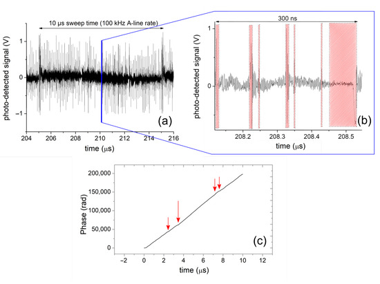
Figure 1.
(a) Channelled spectrum as acquired from the photo-detector in the OCT system with the optical source used in this study. (b) Zoomed version of (a), with the shaded regions denoting the portions of time when the optical frequency is not swept linearly, which are invalid and therefore removed based on the information carried by the data valid vector. (c) Phase of the interferogram (trimmed to one cycle) represented in (a), showing discontinuities (red arrows) pertaining to the portions of time when the optical frequency is not swept linearly.
Master–Slave OCT [9] (MS–OCT) processes the raw OCT data differently. Instead of employing a Fast-Fourier Transform (FFT), MS–OCT performs a comparison of the raw OCT data against either: (i) pre-recorded (or pre-generated) spectra for all axial positions considered [10] or (ii) against “live” spectra provided in real-time by a several optical interferometers using the down-conversion Master–Slave procedure [11] detailed below. Effectively, MS–OCT implements a “calibration” of the system that makes the whole operation tolerant to both the non-linear sweeping [9] as well as to the dispersion left uncompensated in the interferometer [12], enabling swept-source operation without a k-clock [13]. The Vernier tuning enables linear frequency sweeping in time; however, within the sweep there are short, deterministically located regions where the tuning is not linear with the optical frequency. This represents a different set of challenges from those tackled by the MS-based methods in the literature, hence the subject of this paper.
One aspect that is common to all SS-OCT implementations is that the resulting interferometric signal needs to be digitised in order to be processed and the resulting OCT volume rendered. In SS-OCT, the desire or need to image at greater depths demands a larger coherence length for the swept source. The larger the axial range, the higher the sampling rates of the data acquisition system, which drives up costs and electrical power consumption. Furthermore, if the frequency exceeds several GHz, the dynamic range suffers as the available digitizer bit depths for higher sampling rates are 8–10 bit only.
Beyond employing high-speed digitizer cards, other approaches have been reported, such as circular ranging by Siddiqui et al. [14] (the same method improved by Lippok and Vakoc in 2020 [15]) and Chun et al. [16]. This method takes advantage of the aliasing intervals to “unfold” the imaging domain whilst maintaining a lower sampling rate. While this method is advantageous in terms of obtaining a single-shot depth profile, it relies on having single surfaces with no multiple interfaces across the entire “unfolded” imaging range.
Recently, Podoleanu et al. [11] have reported a novel variant of MS–OCT processing, where unlike in the previous MS–OCT paper, the Master and Slave interferometers are two separate physical entities. The comparison operation between the signals returned by them is carried out by using an analogue broadband mixer, prior to digitisation, to mix the signals. The resulting signal is effectively down-converted to frequencies within the order of magnitude of the sweep frequency, enabling the use of lower-speed digitiser cards to acquire the signal and carry out the remainder of operations (signal conditioning and image rendering) digitally.
In this communication, the suitability of MS–OCT is investigated for processing the signal delivered by an OCT interferometer when driven by an electrically tunable, akinetic swept source presenting non-linearities throughout the sweep. In a short preliminary study [17], a demonstration was performed of two of the possibilities of using the MS methods. Here, we expand to more modalities, as presented, and document details of procedures, calibrations, and results, compared with conventional modalities in terms of axial resolution and axial range.
If MS–OCT is proven suitable as a processing method, then a Vernier tuning principle could be used in a simpler manner: there would be no need for a DVV-based correction and, ultimately, no need for an external clock (synchronous with the optical source), thus somewhat simplifying the overall system. Unlike earlier studies with the MS–OCT method, here we compare against a “Master” mask that contains a few non-linearly tuned intervals in the spectrum, which are otherwise eliminated by the DVV calibration. When using the MS–OCT procedure, the entire photo-detected signal is compared against itself; i.e., the signal contains the intervals otherwise eliminated by the DVV correction. We also evaluate the use of the down-conversion OCT method [11], which would bypass the need for both DVV correction (including the synchronous clock) and a high-speed digitiser card to cope with the large frequency of the photo-detected signal. Due to the comparison of spectra that is fundamental to MS–OCT, some tolerance to distorted spectral behaviour should also be expected.
2. Materials and Methods
Throughout this study, an optical source from Insight (model SLE-101) [18], with a sweep rate of and the maximum tuning range setting (roughly ), centred at , is employed.
At the sample clock frequency setting used (), a maximum of 4000 sampling points are enabled at a source sweep duty cycle of 100%. Due to the presence of the invalid regions in the tuned spectrum, the DVV returns useful data within a duty cycle of 70% only. During this study, two separate interferometric setups were employed, which are schematically represented in Figure 2a,b.
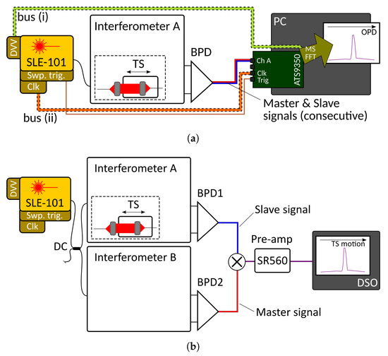
Figure 2.
Schematic diagrams of the two interferometric configurations used with the electrically tunable akinetic optical source throughout this study. (a) Single interferometer configuration, illuminated by the Insight akinetic source SLE-101, driving a balanced photo-detector BPD. (b) Dual interferometer configuration to implement the down-conversion MS–OCT method.
In the first case, as shown in Figure 2a, MS–OCT processing is explored in a single interferometer configuration with a recirculating reference path, following the procedures described by Rivet et al. [10]. Bus (i) carries the DVV produced during the source’s self-calibration, and bus (ii) synchronises the acquisition clock from the digitiser board (ATS9350) with that of the optical source. As shown by the large green arrow in Figure 2a, Master–Slave (MS) or FFT processing can be implemented on the PC. An electronically adjustable translation stage TS (Newport M-VP-25XA) is used to vary the optical path difference (OPD) in the reference arm. The resulting interferometric signal is detected by a balanced photo-detector unit (Insight BPD-1, cut-off frequency ) and digitised using an AlazarTech ATS9350 board (12-bit digitisation bit depth, maximum sampling rate ). For the digitisation procedure, it is possible to use the clock signal provided by the optical source (represented as bus (ii) in Figure 2a), or the built-in hardware clock from the AlazarTech digitiser card (asynchronous clock operation). The DVV correction (bus (i)) is only possible with synchronous clock operation.
In the second case, schematically represented in Figure 2b, the down-conversion OCT (DC-OCT) Master–Slave method [11] was employed on a long axial range (>)-swept source-based system. To achieve this goal, an additional optical interferometer, Interferometer B (Master) was set up with the same optical path difference as Interferometer A presented above (Slave), both having of SMF-28e fibre in their reference arms, which introduces an optical path difference of ≈; these two interferometers were both fed by the Insight source using a 60/40 fused fibre-based directional coupler DC, as depicted in Figure 2b. The outputs of each interferometer are photo-detected by balanced photo-detectors BPD1 (Insight BPD-1) and BPD2 (Thorlabs model PDB481C, AC-coupled, bandwidth –). The resulting electrical signals from either photo-detector are high-pass-filtered (Thorlabs, model EF513, cutoff frequency, not shown in diagram) and directed to a RF frequency mixer, shown as a circled X in the diagram in Figure 2b (Minicircuits, model ZFM-4, operating bandwidth 5–). Its output is first low-pass filtered and amplified (Stanford Research low-noise pre-amplifier, model SR560) and then displayed by a digital storage oscilloscope, DSO (LeCroy model LC534A), running at a sample rate of ∼. To produce an A-scan in this case, the OPD of Interferometer A is varied whilst the DSO reads the filtered output of the pre-amplifier and displays it against time on its screen.
At this very large OPD of ≈, the frequency of the photo-detected signal exceeds . The Nyquist limit of the digitiser board used earlier in the study is (if working with the asynchronous clock of the digitiser board), therefore, the board is not able to sample the resulting interferogram.
2.1. Channelled Spectrum Processing for MS–OCT
To evaluate MS–OCT processing in a single interferometer configuration (Figure 2a), the procedure demonstrated in Rivet et al. [10] is employed, allowing masks to be synthesised from a small set of experimentally acquired channelled spectra. This procedure is schematically represented in Figure 3a. Briefly, during the Master step, a small number of channeled spectra are acquired for several OPD settings and used to infer a pair of system model calibration functions (g and h). These two functions can then be used to render an arbitrary number of complex-valued Master signals, which are then compared against the real-valued channeled spectra acquired during the Slave step, finally generating the full A-scan profile.
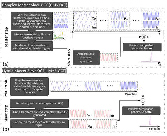
Figure 3.
(a) Simplified description of the Complex Master–Slave OCT procedure presented in Rivet et al. [10]; (b) Diagrammatic description of the hybrid HyMS–OCT method to perform MS–OCT processing of the non-DVV-corrected interferograms retrieved with the akinetic swept source system used in this study.
While the procedure was successfully validated when the interferograms were DVV-corrected (as one would normally use the Insight source), it failed otherwise. This is expected, due to the discontinuities in the phase of the interferogram, as evidenced by the plot in Figure 1c. Moreover, as shown later in Section 3, the frequency spectrum of the interferogram acquired with no DVV correction presents multiple peaks due to the aforementioned discontinuities; since the generation of masks requires a channeled spectrum whose variation in peak density with wavenumber is monotonic, it was not possible to infer the system model calibration functions g and h, as per Figure 3a, and ultimately the complex-valued Master signals. This is not a failure of the MS principle, but rather of the specific algorithm to synthesise masks from experimentally acquired spectra for different OPD values, which has been successfully employed so far on other commercial swept sources.
Instead, a hybrid operation mode was implemented (HyMS–OCT), comprising portions of the original MS–OCT concept [9] but employing complex-valued spectra (as explained in a subsequent paper on MS–OCT, where masks are complex-valued, for which reason such a MS–OCT version denominated CMS–OCT [10]) to enhance the tolerance to phase fluctuations [10].
The hybrid procedure is described diagrammatically in Figure 3b. To obtain an A-scan for a single reflector, the procedure is split into two stages, the Master and the respective Slave. In the Master stage, the reference arm length was varied over the depth range under study using the translation stage TS, whilst constantly retrieving the Master signals, which were then Hilbert-transformed (producing complex-valued spectra) and stored in the computer’s memory. Following this, in the Slave stage, the object under test, considered here a mirror, was positioned in the middle of the depth range under study, and a single Slave signal was acquired. This signal was then compared against the set of Master signals by means of a matrix multiplication, as described in Bradu et al. [19] and the result of these comparisons plotted against the TS position, thus generating an A-scan.
3. Results
Firstly, a frequency characterisation of the interferogram with a single interferometer configuration was performed, for the case where the DVV correction is applied versus the case where the DVV correction is not applied, for two OPD values ( and ), as shown in Figure 4. When the DVV correction is not applied, the invalid signal regions present within the interferometric signal introduce additional frequencies; therefore the red traces in both plots display multiple peaks. These additional frequencies, when not eliminated, degrade the A-scan and also axially move the main A-scan peak from its “true” location.
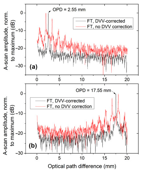
Figure 4.
Comparison of A-scans obtained for two separate OPD values by Fourier-transforming the interferogram ((a) −; (b) −), with (black trace) and without (red trace) DVV correction. Data normalized to the maximum value in each data set, and the logarithmic dB scale on all A-scan profiles was computed with , where is the normalized A-scan profile.
For the first part of the study, described in Section 3.1, the single interferometer configuration (Figure 2a) with a single reflector in the object arm was used, thus generating a single modulation frequency in the interferogram. In the second part of the study (Section 3.2), the dual interferometer configuration of Figure 2b was used, with single reflectors employed as samples in the object arms of either interferometer.
3.1. Complex Master–Slave/Hybrid Master–Slave Operation with Pre-Stored Masks
As mentioned in Section 2.1, any attempts to use the CMS–OCT method described in [10] on any non-DVV-corrected data have proven unsuccessful. The method did work on DVV-corrected interferograms, and the full width at half-maximum (FWHM) for the A-scan peaks was approximately . The transform-limited peak width was also measured as , following the procedure described in Appendix C of Reference [10]. This procedure removes all non-linearities present in the phase, preserving only the spectral shape of the signal; therefore, it yields the minimum width attainable by the system for the tuning range specified.
To study the suitability of the MS–OCT method in non-DVV-corrected cases, complex-valued Master masks were generated using the HyMS–OCT method described in Section 2.1, and compared against a single Slave signal. Similar OPD values to those in Figure 4, of and , were used here, representing a “short” and “large” OPD depth range, respectively. This HyMS–OCT method was evaluated for three sampling/processing protocols as follows:
- Interferogram corrected with the DVV data, having been sampled with the source’s clock signal (both (i) and (ii) buses connected to the digitiser in Figure 2a);
- Interferogram not corrected with the DVV data, but still sampled with the source’s clock signal (bus (ii) only in Figure 2a connected);
- Interferogram sampled with the digitiser card’s built-in clock signal (). Due to the asynchronous operation, the DVV correction is not possible (both (i) and (ii) buses in Figure 2a disconnected).
For these three sampling/processing protocols, A-scans were obtained by comparing the Slave signal corresponding to a reflector placed in the middle of the depth range intervals under study (corresponding to a “short” and “large” OPD range, both spanning ) against a pre-recorded, complex-valued set of Master signals recorded over the same depth range interval, using a matrix multiplication, as described in Bradu et al. [19]. The result of these comparisons is plotted against the TS position, thus generating A-scan profiles as depicted in Figure 5a,b alongside those obtained by Fourier transforming the DVV-corrected interferograms.
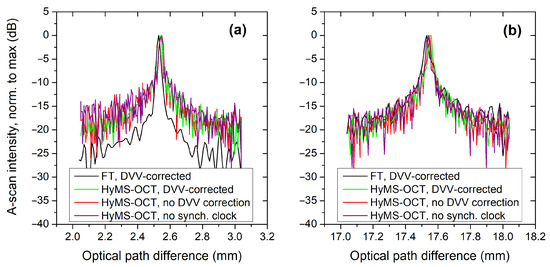
Figure 5.
A-scans for three sampling cases as detailed in the insets taken at small (≈2–) (a) and large (≈17–) (b) OPD values with the HyMS–OCT method for the different sampling cases considered. The conventional procedure, the Fourier transform of the DVV-corrected interferogram, is plotted in black in both graphs.
As Figure 5a,b show, the A-scan profiles obtained with the HyMS–OCT method on all sampling/processing protocols are very similar, both in terms of peak width and S/N ratio. In other words, the HyMS–OCT method works equally well with DVV-corrected and DVV-uncorrected data.
The location of the A-scan peaks obtained with the FT processing differs slightly from those obtained with the HyMS–OCT due to the different manner the OPD coordinate is determined: in the FT processing, the full A-scan profile needs to be mapped to the distance coordinate by taking several position measurements and interpolating the distance between them, which introduced some imprecision. In the HyMS–OCT processing, each Master signal is directly mapped to a single position of the TS, effectively providing an absolute calibration of each depth point.
The FWHM of all peaks plotted in Figure 5 are listed in Table 1 and Table 2, and their corresponding signal-to-noise ratio values in Table 3 and in the second column of Table 2. These contain the FHWM peak values from the DVV-corrected interferograms and from the non-DVV corrected ones, respectively.

Table 1.
Full-width at half-maximum values of the A-scan peaks (in ) for the methods evaluated for a short () and a large () OPD value, employing DVV-corrected data. No spectral windowing was employed in any of interferograms used to obtain these A-scan peaks.
Table 2.
Full-width at half-maximum values of the A-scan peaks (in ) and their respective signal-to-noise ratio (SNR) values (in dB) for the HyMS–OCT method, employing data sampled without DVV correction. No spectral windowing was employed in any of the interferograms used to obtain these A-scan peaks.
Table 3.
Signal-to-noise ratios (SNR) of the A-scan peaks (in dB) for the methods evaluated for a short () and a large () OPD value, employing DVV-corrected data. No spectral windowing was employed in any of interferograms used to obtain these A-scan peaks.
Regarding the peak width values obtained with the FFT method, it is clear that for the two OPD values considered, larger widths than the expected transform-limited value are obtained. For the larger OPD value (≈), the peak width is significantly larger, and a depth-dependent widening is observed. Since the interferometer used in this study was not fully compensated for material dispersion between its two arms, this result is to be expected. This depth-dependent widening is not observed in the results obtained with either CMS–OCT or HyMS–OCT since the MS–OCT method automatically compensates [12] for any material dispersion imbalance in the system.
The CMS method employing synthesised complex-valued masks provides the closest peak width value to the transform-limited width (the ground truth), differing by less than in the short OPD case.
The last column of Table 1 and the middle column of Table 2 relate to peak width values obtained using the HyMS–OCT method employing pre-recorded Master masks, as described in Section 2.1. In this case, the peak width was estimated from a shorter run of the TS (500 points over a travel range of ≈, centred at the relevant OPD where the Slave signal was acquired). The larger values (when compared with those obtained for the CMS–OCT method employing synthesised complex-valued masks) may be due to the precision limitations of the mechanical translation stage encoder, and the settling time allowed for each individual position recording of the channelled spectra. Still, it is clear that no depth-dependent peak widening is observed when using the HyMS–OCT method, as shown in Table 1 and Table 2. For most cases, the peak widths are smaller than those obtained with the FFT method.
In Table 2, the peak widths for the HyMS–OCT under asynchronous clock operation between source and digitizer are only slightly larger (by ≈) than the other two cases obtained with the same processing method; this is due to the fact that the digitiser used has fixed, pre-set clock settings that do not match the clock signal frequency used in the other two cases (). In this particular case, the maximum clock frequency allowed by the digitiser card, , was used, but the number of sampled points was kept constant. This has an impact in terms of the sampled region of the spectrum, with the digitised spectral range not fully covering the sweep range of the source, which was expected to negatively impact the axial resolution measured.
We present the signal-to-noise ratio (SNR) values for the A-scan peaks in Figure 5a,b in Table 2 and Table 3. These SNR values should be interpreted with some reservation, as they represent single run events and no average or detailed noise analysis was performed. Data employed in the SNR calculations were collected in separate events. This may explain some variations in the values presented. To avoid signal saturation, a different attenuation of the reference power was applied when switching from one regime to another, which was maintained consistently for measurements on each regime for different OPD values, for instance, but not when switching between regimes.
In both Table 2 and Table 3, the larger the OPD value for both CMS–OCT and HyMS–OCT methods, the larger the SNR, despite the system sensitivity decreasing with OPD, showing that noise decreases at a higher rate than the sensitivity when moving to larger RF frequency values. There might be other noise components with larger strength at smaller RF frequency values (shallow OPD values) that may explain this. As far as the FFT case, the noise floor lies more than 5 dB below the noise floor of the other three traces at short OPD values. The trend of S/N noise with OPD cannot be commented on for the FFT data as no dispersion compensation was applied.
To study the applicability of the HyMS–OCT method to large axial range measurements, an A-scan was produced over the full range of OPD values allowed by the sampling clock from the digitiser card for the locations where the two Slave signals were previously recorded. This behaviour was tested for the case with asynchronous clock operation between source and digitiser (operating at , which translates into ≈ of depth range, with of it represented in the plot). The resulting A-scans were compared against those obtained from FFT processing of the interferogram, with and without DVV correction. These results are shown in Figure 6.
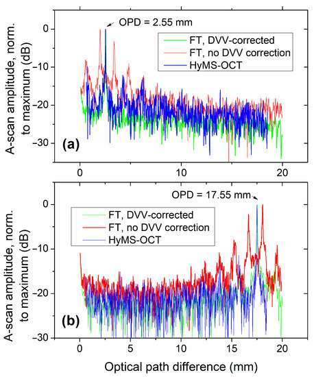
Figure 6.
A-scan comparison between the FT method (on both DVV and non-DVV corrected interferograms) and the HyMS–OCT method (asynchronous clock case, no DVV correction), for a total OPD value scan range of . Arrows depict the corresponding OPD at which the Slave signal was acquired for the two sub-figures ((a) −; (b) −), and also the OPD values of the interferograms subject to FT processing.
As expected, if the non-DVV-corrected interferogram is processed using the FFT method, not only is there a rise in the noise floor level, but also the appearance of satellite peaks, whose heights are comparable to those of the main interferometric peak, as has already been shown in Figure 4. The trace corresponding to the non-DVV corrected, HyMS–OCT-processed interferogram also presents some residual satellite peaks, although these are significantly reduced when compared to those present in the non-DVV-corrected, FFT-processed trace, being attenuated by more than dB.
The noise floor behaviour mimics what was presented before: the DVV-corrected interferogram, when processed using the FFT method, possesses a lower noise floor (by about dB) when compared to the same data processed using the HyMS–OCT method (without DVV correction, and without using the clock signal from the source). However at a larger OPD value, closer to the sampling limit of the digitiser, the difference between the noise floor of the DVV-corrected, FFT-processed interferogram and that processed using the HyMS–OCT method is not significant, possibly due to the fact that no dispersion compensation was applied on the FFT-processed data, as mentioned earlier.
No S/N ratio value is presented for the coherence limited peak in Table 3, as this is obtained from the envelope of the spectrum, that is similar to that obtained from the reference or sample wave only. In other words, we cannot associate a separate signal or noise measurement to this procedure (signal in OCT is measured with both waves on and noise with the sample wave obstructed).
Since the primary concern with this study was to assess any peak width degradation when using any of the methods evaluated, no spectral windowing was applied to any of the interferograms processed, which may explain the existence of side-lobes in some of the A-scans presented in Figure 4, Figure 5 and Figure 6.
3.2. Down-Conversion (DC) OCT Implementation with Two Physical Interferometers
To evaluate the axial resolution with the DC-OCT method, the OPD in one of the two interferometers is scanned mechanically using the TS in Interferometer A, as presented in Section 2. This leads to the graph in Figure 7. This is not, however, the way the DC-OCT method is normally used, where no mechanical depth scanning is applied; as demonstrated by Podoleanu et al. [11], DC-OCT allows the production of constant depth images of the object under study (en-face images) by setting both interferometers to the same optical path difference and comparing the channelled spectra of similar modulation.
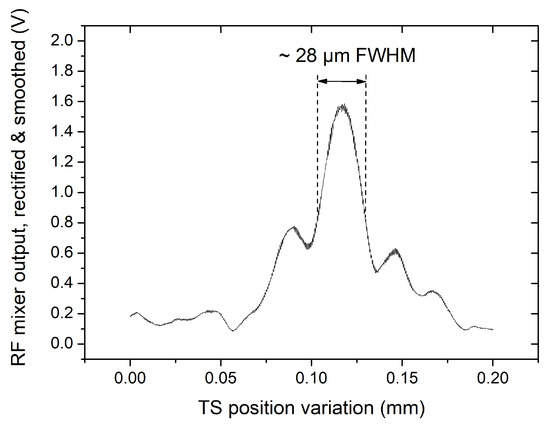
Figure 7.
A-scan obtained with the down-conversion procedure, with the Master interferometer having an OPD value of ∼, and the reference arm of the Slave interferometer being mechanically scanned over a range of at ∼ OPD. The main peak has a FWHM of ∼, which corresponds to an axial resolution of ∼ due to the double-pass interferometer configuration.
The second interrogating interferometer performs real-time generation of the mask, therefore operating as an Optical Master. In contrast, in all previous MS papers, masks were generated electrically and/or numerically by Electronic Masters, and then stored in the PC memory.
A down-conversion factor N can be calculated as the ratio between the frequency of the photo-detected signal for the maximum OPD recoverable and the frequency of the processor performing the down-conversion (composed of the mixer and the low-pass filter). Considering the Nyquist limit, this should be at least twice the sweep frequency value, therefore giving a value of . This means that by using DC-OCT, the bandwidth of photo-detected signal was reduced by a factor of 3000. The A-scan peak obtained using the down-conversion method exhibits a width of ≈, slightly larger than the expected .
4. Discussion and Conclusions
This study has evaluated the suitability of three versions of the MS–OCT method to decode interferograms, delivered by an interferometer driven by an electrically tunable (Vernier tuning) swept source that presents invalid regions throughout its tuning. The three MS–OCT versions are as follows: (i) using pre-synthesised, complex-valued masks (CMS–OCT); (ii) a hybrid (HyMS–OCT) modality, where multiple Master masks are generated by multiple stepped OPD changes and compared against a complex-valued Slave signal; and (iii) a DC-OCT version. As demonstrated, both (ii) and (iii) methods can be used with some success, even when interferograms are not corrected by the manufacturer’s DVV. The CMS–OCT method with pre-synthesised masks can only work with DVV-corrected spectra. Therefore, the MS–OCT methods present a suitable alternative for the signal processing of OCT systems driven by swept sources employing a similar tuning modality as that of the Insight source used in this study. If the use of a DVV correction can be eliminated, as allowed by both (ii) and (iii) methods, signal processing is simplified with an overall cost advantage for the whole OCT system. A summary of the advantages (and disadvantages) of the approaches presented in this study is shown in Table 4.
Table 4.
Summary of positive and negative aspects of using the MS–OCT method with the akinetic, electrically tunable swept source employed in this study.
One of the advantages of the electrically tunable source used in this study is its long axial range, which can be on the order of tens of centimetres or more; in order to digitise such interferograms, ultra-fast digitiser cards with multi- sampling clocks are needed. However, if the DC procedure presented in this study (and detailed by Podoleanu et al. [11]) is used, one can do without the digitiser card altogether. In effect, this has also been demonstrated in this study, where an A-scan taken at an OPD value of is obtained, which would have otherwise been impossible to obtain with the ATS-9350 digitiser card, as the OPD corresponds to a dominant channelled spectrum frequency of more than over the digitiser’s aliasing limit. This conclusion can be scaled to larger frequency sweeping rates, exceeding tens of , where the DC procedure would allow processing of tens of GHz-frequency signals using digitisers with sampling rates in the range of the sweeping rate.
As demonstrated, the method described by Rivet et al. [10] to pre-synthesise the Master signals for the CMS–OCT procedure is only applicable to the case where the DVV correction is applied. However, the DVV correction and external clock sampling only address one of the issues encountered with SS-OCT, that of securing linear sweeping. The other issue is the dispersion in the interferometer. The MS calibration addresses both non-linear sweeping and dispersion. Therefore, when compared with the conventional usage case of these optical sources (DVV correction followed by FT), the MS procedure presented here offers some benefit, in the sense that it is tolerant to dispersion in the system [12]. This is demonstrated in Table 1 by the improvement in the peak width brought by the CMS–OCT with synthesised masks when compared against that obtained by simple FFT.
The HyMS–OCT procedure with non-DVV-corrected interferograms was made working with pre-recorded spectra. A similar approach was used in the earlier MS–OCT implementations [9,12], and while it worked well enough for the demonstrations, it has a negative impact on the flexibility and usability of the system, as a large number of masks need to be collected. The procedure for synthesising the masks from a small sub-set of channelled spectra, however, can potentially be upgraded to something more tolerant of the extra frequency terms (e.g., by suppressing the satellite terms during capture using band-pass filtering). More research will need to be carried out with regards to this aspect.
Running the HyMS–OCT procedure on non-DVV-corrected data appears to raise the noise floor, especially when imaging at lower OPD values; moreover, some satellite terms, similar to those observed when Fourier-transforming a non-DVV-corrected interferogram, also appear in the A-scan, albeit significantly attenuated. This could pose a problem, especially if low-bit-depth digitiser cards are used, as they will present lower dynamic range in the digitisation. Still, bypassing the requirement for DVV correction means that the need for synchronous sampling operation between source and digitiser is eliminated, with potential cost savings and additional flexibility. For example, with a sufficiently large sampling rate digitiser, OPD values beyond the limit introduced by the source clock can be accessed, as has already been demonstrated in Marques et al. [13].
In the second part of this study, the operation of this optical source without the need for a high-speed digitiser was also investigated, by means of the down-conversion OCT method [11]. By using two near-identical optical interferometers and mixing their output interferograms with an analogue RF mixer, long-range operation at an OPD value of is demonstrated. When compared with the results from the first part of our study, the axial resolution obtained was not significantly deteriorated. Indeed, it actually presented a > improvement over the width measured for DVV-corrected, FT-processed data at .
The peak width is, however, slightly larger than all results obtained using the CMS/HyMS–OCT procedures. This is explained by some dispersion difference between the two optical interferometers. Moreover, it was not possible to perform any spectral windowing on these time-based signals, which can also explain the presence of side-lobes in the A-scan.
The peak contrast is also significantly reduced, to less than dB, compared with the ≈ dB obtained with the CMS/HyMS–OCT procedures. The bandwidth of the Insight BPD-1 (employed in the Slave interferometer), narrower than the Thorlabs photo-detector employed in the Master interferometer, explains the lower peak contrast at large OPD values.
This is only a constructive disadvantage due to the non-availability of two balanced photo-detectors. Even so, DC-OCT is worth pursuing due to the lowering of the signal processing bandwidth to levels comparable to the sweeping frequency. This allows a low-cost route via low-cost digitizers, a procedure that also enables real-time delivery capability of en-face views, as when using ultra-high-speed digitizers, the amount of data is so high that it needs to be buffered locally before being transferred out of the digitizer for post-acquisition. The more important disadvantage of DC-OCT is the need for a second high-speed, large-bandwidth photo-detector unit.
In summary, Master–Slave OCT (both in its HyMS–OCT and DC-OCT guises) offers some simplification over the conventional DVV-based invalid region removal procedure, allowing the user to employ both the valid and invalid regions, as long as a reference interferometer (Master) signal is available (either pre-stored at a Master step or as a physical interferometer as in the down-conversion case). Another advantage of the MS approach is that it may enable better analysis of phase errors, particularly at higher imaging depths. These phase errors may occur around the invalid-to-valid transitions due to slight imperfections in the discontinuity resolution with the DVV or simply due to a change in the performance of the laser over time or ambient temperature.
Author Contributions
Conceptualization, A.P. and M.J.M.; methodology, A.P. and M.J.M.; software, M.J.M. and A.B.; validation, M.J.M. and R.C.; formal analysis, M.J.M.; investigation, M.J.M. and R.C.; resources, A.P. and J.E.; data curation, M.J.M.; writing—original draft preparation, M.J.M.; writing—review and editing, M.J.M., R.C., J.E., A.B., and A.P.; visualization, M.J.M.; supervision, A.P. and A.B.; project administration, A.P.; funding acquisition, A.P. and A.B. All authors have read and agreed to the published version of the manuscript.
Funding
A. Podoleanu, A. Bradu, and M. J. Marques are supported by the Biotechnology and Biological Sciences Research Council (BBSRC) (5DHiResE, BB/S016643/1) and the Engineering and Physical Sciences Research Council (EPSRC) (REBOT, EP/N019229/1). M. J. Marques and A. Podoleanu acknowledge support from the Image Guided Therapy EPSRC Plus Network, EP/N027078/1. A. Podoleanu and R. Cernat acknowledge the support of National Institute for Health Research (NIHR) Biomedical Research Centre at the UCL Institute of Ophthalmology, University College London, the Moorfields Eye Hospital NHS Foundation Trust, and the NETLAS Marie-Curie ITN 860807. A. Podoleanu also acknowledges the Royal Society Wolfson research merit award.
Acknowledgments
The authors are grateful to Insight Corporation for the loan of the Insight SLE-101 necessary for this study. The authors also thank Sally Makin for the thorough readability review prior to submission.
Conflicts of Interest
A.P. and A.B. are inventors of patents: US10760893 and US9383187 in the name of the University of Kent. R.C. and M.J.M., no conflicts of interest. J.E. is the chief technological officer (CTO) and executive vice-president (EVP) of Insight Photonic Solutions, Inc. The funders had no role in the design of the study; in the collection, analyses, or interpretation of data; in the writing of the manuscript, or in the decision to publish the results.
References
- Swanson, E.A. OCT Technology Transfer and the OCT Market. In Optical Coherence Tomography: Technology and Applications; Drexler, W., Fujimoto, J.G., Eds.; Springer International Publishing: Cham, Switzerland, 2015; pp. 2529–2571. [Google Scholar] [CrossRef]
- Leitgeb, R.; Hitzenberger, C.; Fercher, A. Performance of fourier domain vs. time domain optical coherence tomography. Opt. Express 2003, 11, 889. [Google Scholar] [CrossRef] [PubMed]
- Minneman, M.P.; Ensher, J.; Crawford, M.; Derickson, D. All-Semiconductor High-Speed Akinetic Swept-Source for OCT. In Optical Sensors and Biophotonics; Paper 831116; Optical Society of America: Shanghai, China, 2011; p. 831116. [Google Scholar] [CrossRef]
- Wang, Z.; Potsaid, B.; Chen, L.; Doerr, C.; Lee, H.C.; Nielson, T.; Jayaraman, V.; Cable, A.E.; Swanson, E.; Fujimoto, J.G. Cubic meter volume optical coherence tomography. Optica 2016, 3, 1496. [Google Scholar] [CrossRef] [PubMed]
- Park, J.; Carbajal, E.F.; Chen, X.; Oghalai, J.S.; Applegate, B.E. Phase-sensitive optical coherence tomography using an Vernier-tuned distributed Bragg reflector swept laser in the mouse middle ear. Opt. Lett. 2014, 39, 6233–6236. [Google Scholar] [CrossRef] [PubMed]
- MacDougall, D.; Farrell, J.; Brown, J.; Bance, M.; Adamson, R. Long-range, wide-field swept-source optical coherence tomography with GPU accelerated digital lock-in Doppler vibrography for real-time, middle ear diagnostics. Biomed. Opt. Express 2016, 7, 4621–4635. [Google Scholar] [CrossRef] [PubMed]
- Song, S.; Xu, J.; Wang, R.K. Long-range and wide field of view optical coherence tomography for in vivo 3D imaging of large volume object based on akinetic programmable swept source. Biomed. Opt. Express 2016, 7, 4734–4748. [Google Scholar] [CrossRef] [PubMed]
- Salas, M.; Augustin, M.; Felberer, F.; Wartak, A.; Laslandes, M.; Ginner, L.; Niederleithner, M.; Ensher, J.; Minneman, M.P.; Leitgeb, R.A.; et al. Compact akinetic swept source optical coherence tomography angiography at 1060 nm supporting a wide field of view and adaptive optics imaging modes of the posterior eye. Biomed. Opt. Express 2018, 9, 1871–1892. [Google Scholar] [CrossRef] [PubMed]
- Podoleanu, A.G.; Bradu, A. Master–slave interferometry for parallel spectral domain interferometry sensing and versatile 3D optical coherence tomography. Opt. Express 2013, 21, 19324. [Google Scholar] [CrossRef] [PubMed]
- Rivet, S.; Maria, M.; Bradu, A.; Feuchter, T.; Leick, L.; Podoleanu, A. Complex master slave interferometry. Opt. Express 2016, 24, 2885. [Google Scholar] [CrossRef] [PubMed]
- Podoleanu, A.; Cernat, R.; Bradu, A. Down-conversion en-face optical coherence tomography. Biomed. Opt. Express 2019, 10, 772. [Google Scholar] [CrossRef] [PubMed]
- Bradu, A.; Maria, M.; Podoleanu, A.G. Demonstration of tolerance to dispersion of master/slave interferometry. Opt. Express 2015, 23, 14148. [Google Scholar] [CrossRef] [PubMed]
- Marques, M.J.; Rivet, S.; Bradu, A.; Podoleanu, A. Complex master-slave for long axial range swept-source optical coherence tomography. OSA Contin. 2018, 1, 1251. [Google Scholar] [CrossRef]
- Siddiqui, M.; Nam, A.S.; Tozburun, S.; Lippok, N.; Blatter, C.; Vakoc, B.J. High-speed optical coherence tomography by circular interferometric ranging. Nat. Photonics 2018, 12, 111–116. [Google Scholar] [CrossRef] [PubMed]
- Lippok, N.; Lippok, N.; Vakoc, B.J.; Vakoc, B.J.; Vakoc, B.J. Resolving absolute depth in circular-ranging optical coherence tomography by using a degenerate frequency comb. Opt. Lett. 2020, 45, 371–374. [Google Scholar] [CrossRef] [PubMed]
- Chun, S.K.; Jang, H.; Cho, S.W.; Park, N.S.; Kim, C.S. Unfolding displacement measurement method for the aliasing interferometer signal of a wavelength-comb-swept laser. Opt. Express 2018, 26, 5789–5799. [Google Scholar] [CrossRef] [PubMed]
- Marques, M.J.; Cernat, R.; Ensher, J.; Bradu, A.; Podoleanu, A. Master-slave principle applied to an electrically tunable swept source-OCT system. In Optical Coherence Tomography and Coherence Domain Optical Methods in Biomedicine XXIV; International Society for Optics and Photonics: San Francisco, CA, USA, 2020; Volume 11228, p. 112280D. [Google Scholar] [CrossRef]
- Insight Akinetic Swept Lasers Enabling OCT and SS-OCT Angiography|Insight. Available online: https://www.sweptlaser.com/content/insight-akinetic-swept-lasers-enabling-oct-and-ss-oct-angiography (accessed on 27 May 2020).
- Bradu, A.; Rivet, S.; Podoleanu, A. Master/slave interferometry – ideal tool for coherence revival swept source optical coherence tomography. Biomed. Opt. Express 2016, 7, 2453. [Google Scholar] [CrossRef] [PubMed]
Publisher’s Note: MDPI stays neutral with regard to jurisdictional claims in published maps and institutional affiliations. |
© 2021 by the authors. Licensee MDPI, Basel, Switzerland. This article is an open access article distributed under the terms and conditions of the Creative Commons Attribution (CC BY) license (https://creativecommons.org/licenses/by/4.0/).