1. Introduction
Lidar has gradually become a promising means of environmental perception compared with traditional microwave radar due to its superior spatial and temporal resolution and the advantages of being less restricted by weather and lighting conditions. Especially photon counting lidar, due to its extremely high detection sensitivity, has attracted wide attention from researchers and has broad application prospects in the fields of ranging, three-dimensional imaging, target tracking and recognition, and mapping [
1,
2,
3,
4,
5]. However, because the traditional photon counting lidar emits pulses with a fixed repetition frequency [
6], the periodicity and regularity of the pulses will not only cause range ambiguity but are also vulnerable to interference and jamming. Especially in the near future, with the intensive application of lidar, it will be inevitable to receive signals from other lidars. In this case, the lidar will be affected by crosstalk, which will lead to the failure of detection [
7,
8]. Therefore, lidar should not only have high ranging accuracy and long ranging capability but also have strong anti-interference ability to meet the application requirements of complex scenarios in the future.
To mitigate the possibility of interference, modulation coded lidars have been studied. Lidar systems with different aperiodic or irregular laser pulse modulation schemes, such as the pseudo-random modulation [
8,
9,
10] and the chaotic pulse position modulation (CPPM) have been studied [
11,
12,
13,
14,
15]. However, the pseudo-random modulation sequence is periodic and reproducible, so a malicious jammer can easily record the transmitting pseudo-random modulation sequence and then re-transmit it to generate false echo to interfere with the lidar [
12]. The CPPM sequence generated by chaotic map is susceptive to the change in parameters [
15], and the chaotic pulse sequence generated based on the optical feedback method is complex and low in efficiency.
In 2020, our previous work and Tsai almost simultaneously published a study on a new modulation method. In this method, Gm-APDs (Geiger-mode of Avalanche Photodiode) is used as random signal generators to generate true nature-based random sequences [
16,
17,
18]. This true random modulation method has higher anti-interference immunity than the pseudo-random modulation method because the true random sequence generated based on Gm-APD is essentially a kind of digital noise, which is not repeatable and non- reproducible.
The peculiarity of this paper is using Gm-APD to generate true random sequence, which has strong anti-interference ability. Compared with Pseudorandom Noise (PN) sequence, it also has the advantage of overcoming the influence of Gm-APD dead time. For PN sequences, the interval between two adjacent ‘1’ codes is less than the Gm-APD’s dead time. When the Gm-APD’s responds to a photon, it will enter the dead zone and cannot respond to any other arriving photons. Thus, when a ‘1’ code of the PN sequence is responded, Gm-APD enters the dead zone, and any ‘1’ code in the subsequent pseudorandom sequence cannot be responded until Gm-APD recovers from the dead zone [
19,
20,
21]. Therefore, the ranging performance is degraded. For our method, a Gm-APD will not generate any pulse during its dead time, which means that the output pulse interval between any two adjacent pulses is larger than its dead time. Consequently, we can consider that any two ‘1’ codes in the true random sequence are independent of each other [
17,
18]. In this case, the dead time effect can be completely avoided. The detection performance of true random coding photon counting lidar can be obviously improved.
Compared with the chaotic pulse position modulation method, the true random modulation method only needs one Gm-APD to generate a stable true random sequence. Moreover, the generated true random sequence can be directly used to drive the laser source to generate true random optical pulse sequence. The system is simpler than that of the chaotic pulse position modulation method.
In short, the true random coding photon counting lidar based on Gm-APD has the advantages of being a simple system and having a strong anti-crosstalk ability.
Tsai and Hwang verified that Gm-APD can not only produce high-quality random sequences, but also, the generated sequences have strong interference suppression capabilities [
16,
22,
23]. Yu established the theoretical model of transmitting and receiving signals of the photon counting lidar system based on Gm-APD random coding, gave the function model of using system parameters to characterize the true random sequence autocorrelation, and preliminarily verified the detection performance of the system [
18]. In addition, Liu’s experiments verify the ranging and imaging ability of the system [
17].
Although it has been proved that the true random coding photon counting lidar based on Gm-APD has a strong crosstalk suppression ability, and the experiment verifies the ranging imaging ability, References [
16,
17,
18] do not provide a detailed analysis of the detection performance. This paper analyzes its detection performance in detail. The theory model of correct ranging probability is established based on the photon counting statistics theory and considers the influence of jitter on the correct ranging probability, for the first time. The effects of mean echo photon number, sequence length, mean pulse count density, and pulse width on the correct ranging probability are discussed, and the correctness of the correct ranging probability model is verified by Monte Carlo simulation and experiments. Due to the existence of Poisson distribution noise, the echo intensity of each code is not equal. Therefore, we use the mean echo photon number of multiple codes to represent the echo intensity of the system. The sequence length is determined by the period of the external trigger signal. The number of ‘1’ code in the true random sequence per second is defined as the density of the ‘1’ code, which is called the mean pulse count density. The width of the code is defined as the pulse width. The correct ranging probability theoretical model can quantitatively describe the detection performance and provide a solid foundation for further research.
In addition, the correct ranging probability theoretical model provides a theoretical basis for the determination of system parameters such as sequence length, mean pulse count density, single pulse energy, etc. For example, since Gm-APD cannot respond to the echo signal intensity, photon counting lidar usually improves the correct ranging probability of the system by increasing the number of accumulated pulses. An excessive increase in the number of accumulated pulses will reduce the detection speed of the system. Based on the established theoretical model, the minimum detection threshold can be determined according to other known parameters (mean pulse count density, single pulse energy, pulse width, noise level (the mean number of noise photons within each code width), etc.) under the premise of ensuring the correct ranging probability. Then, further determine the minimum sequence length to improve the system detection speed.
2. System Structure and Ranging Principle
This part introduces the system structure and ranging principle of the true random coding photon counting lidar. In this method, a Gm-APD is used as a random signal generator to generate true nature-based random sequences. More research results can read our previous work, such as the system structure, working principle, and the experimental results of ranging imaging [
17,
18].
Figure 1 is the system structure diagram.
The system provides timing benchmarks through external trigger sources. We use FPGA as external trigger source to generate periodic trigger signals. If we use the output signal of PIN (P-region, I-region and N-region (PIN)) detector as the trigger signal, the emitted true random sequence will be recorded as discrete pulses because each code element in the true random sequence will become the start signal, resulting in sequence retiming, and cannot guarantee that the whole true random sequence is recorded as a whole. To ensure that all code elements in a sequence have the same timing benchmark, we add an external trigger module to implement this function. The Gm-APD1 continuously generates digital electrical noise, which can be regarded as a true nature-based random sequence. The external trigger signal is equivalent to providing a gating signal for Gm-APD1 to control the sequence length of the true random signal. After pulse shaping circuit, the true random sequence generated by Gm-APD1 directly drives the laser source to obtain the true random optical pulse sequence. The high voltage of the digital electrical noise sequence is recorded as the ‘1’ code, and the low voltage is recorded as the ‘0’ code. The true random laser pulses sequence is divided into two parts by a ratio beam splitter: one small part of the energy is detected by a PIN detector, which is used as the transmitted reference signal, recorded as
by TCSPC (time-correlated single photon counting) module, and most of the energy is transmitted to the target. The echo signal is detected by Gm-APD2 and is recorded as
by the TCSPC module by calculating the cross-correlation between the echo signal and the emission template, as shown in
Figure 2a [
18]. The correlation function is similar to Dirac delta function,
, where
is code width. When
corresponds to the ToF (Time of Flight), the correlation function
has max value. The target distance can be determined while unwanted signals from other sources only contribute to noise, as shown in
Figure 2b. Code width (pulse width) is the basic matching unit of correlation operation. Therefore, the resolution of true random coded photon counting lidar is still determined by the pulse width.
3. Theoretical Model of Correct Ranging Probability
Correct ranging probability is an important index to evaluate the detection performance of photon counting lidar [
17,
18]. The same is true for true random coding photon counting lidar. The correct ranging probability theoretical model can quantitatively evaluate the system performance and provide the basis for the selection of system parameters. Many parameters and definitions are used in this manuscript. For the convenience of reading, the main parameters and definitions are listed in the
Table A1.
Since the true random sequence is generated by Gm-APD1, as long as the dead time of Gm-APD1 is not less than Gm-APD2, the ‘1’ codes in the true random sequence are independent of each other for Gm-APD2 [
18]. Since the dead time of Gm-APD is determined by the quenching circuit, the dead time of Gm-APD1 can be longer than that of Gm-APD2 by reasonably designing the quenching circuit. Based on the premise that the ‘1’ codes are mutually independent, the correct ranging probability model of true random coding photon counting lidar can be established by referring to the pulse accumulation method. The model mainly includes two core parameters: the correct ranging probability of single ‘1’ code (
) (we define this probability as the counting probability) and the signal recognition threshold (
k). The signal recognition threshold
k can be considered as the detected codes number in the transmitting true random sequence.
3.1. Count Probability
Since the count probability is the same as that of a single pulse, the count probability can be expressed as [
24]
where
is mean noise photoelectron flux,
is mean signal photoelectron flux,
is the dead time of Gm-APD2,
is the time bin width. The time bin width is equal to the time resolution of TCSPC module. The bins width affects the timing accuracy of the echo signal.
3.2. Signal Recognition Threshold
In the true random coding photon counting lidar system, we define the signal recognition threshold as the minimum detected number of ‘1’ codes when the target position can be correctly extracted. When the signal recognition threshold is too high, the system will have obvious missing detection. While when the signal recognition threshold is relatively small, the system will have obvious incorrect ranging. However, when the signal recognition threshold is reasonable, it should be in the critical state.
Firstly, we establish the incorrect ranging probability model of true random coded photon counting lidar. Then, the most reasonable signal recognition threshold can be determined by making the incorrect ranging probability greater than 0 and less than 100%. Assuming that the length of the sequence is
and the average pulse count density of ‘1’ code in the sequence is
.
is transmitted codes number in the sequence. The average pulse interval of each ‘1’ code is
. The detection probability of noise in each pulse width is
. For convenience of analysis, the width of the time bin is set to the pulse width, and
is the number of codes contained in the average pulse interval, where
. When the threshold value is
, the incorrect ranging probability
can be expressed as
when incorrect ranging occurs, it means that at least
k noise counts have the same arrangement as the pulse sequence that occurred. Therefore, we use the average pulse interval of the transmitted true random sequence as the division unit, divide the entire sequence, then calculate the probability of having the same arrangement as the transmitted sequence, and add up the probability of all noise counts greater than
k to obtain the total false alarm probability.
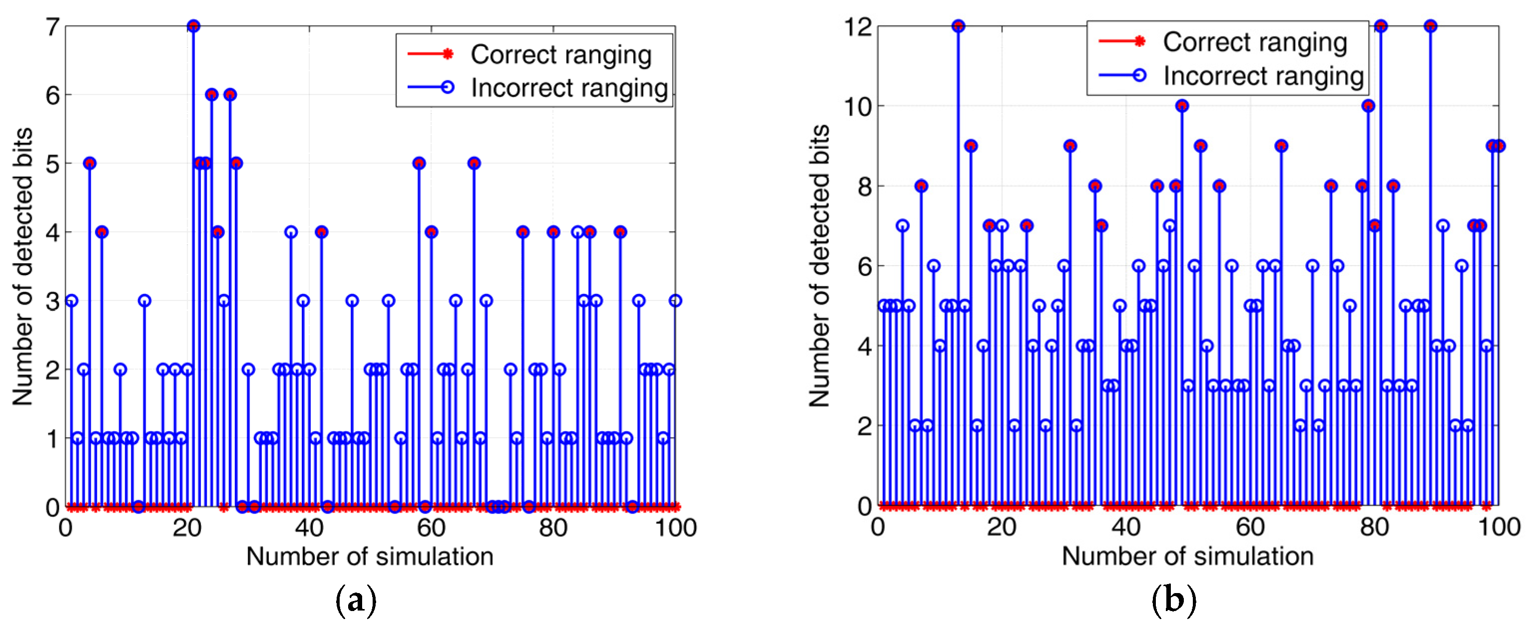
Figure 3a,b shows the results of 100 Monte Carlo simulations of the true random coding photon counting lidar. Each line represents the detected codes number at the correlation operation peak position. The hollow point represents the simulation of incorrectly identifying the target position, that is, the case of incorrect ranging. The corresponding ordinate is the detected noise codes number. The solid red dot indicates the correct recognition of the target position. Its corresponding ordinate represents the detected number of ‘1’ codes.
The sequence length in
Figure 3a is 100 μs, and the sequence length in
Figure 3b is 500 μs. The mean pulse count density, the mean echo photon number, and the noise count level of the two sequences were 1 Mcps, 0.5, and 1 Mcps, respectively. Taking
Figure 3a as an example, when the signal recognition threshold is set to 3, there will be incorrect ranging detections, and when the signal recognition threshold is set to 5, there will be many missing detections. For
Figure 3a, the most reasonable signal recognition threshold should be 4. There are both correct detections and incorrect detections. That is, the incorrect ranging probability is greater than 0 and less than 100%. Therefore, the most reasonable signal recognition threshold can be determined by calculating the
k value which makes the incorrect ranging probability between 0 and 100%.
3.3. Probability of Detected Codes Number Equal to Signal Recognition Threshold
The number of detected codes (i) equal to the signal recognition threshold (k) can be divided into two cases: the number of detected signal ‘1’ codes equal to the signal recognition threshold and the number of detected noise codes equal to the signal recognition threshold. For the first case: when the number of detected ‘1’ codes equals the signal recognition threshold, the target location is not always correctly extracted. There is a chance that noise codes will coincidentally align and equals the threshold, then it will be two correlation peaks, which will cause incorrect detection. For the second case, when the number of detected noise codes is equal to the signal recognition threshold, this detection is certainly incorrect detection. Therefore, it is difficult to directly calculate the correct ranging probability () for the first case. However, the incorrect ranging probability () can be analytically expressed by calculating the probability of noise codes. The incorrect ranging probability means that the number of detected noise code elements (in) is equal to or greater than the signal recognition threshold, in other words in ≥ k. Then, if we know the relationship between the incorrect ranging probability and the correct ranging probability when the detected codes number is equal to the signal recognition threshold, the correct ranging probability can also be quantitatively described.
In order to determine the quantitative relationship between the incorrect ranging probability and correct ranging probability under the signal recognition threshold, we conducted a Monte Carlo simulation. The relationship is simulated under different system parameters (sequence length, mean pulse count density, and noise count level), as shown in
Table 1,
Table 2 and
Table 3. Sequence length changes from 100 μs:50 μs:500 μs. The results are shown in
Table 1 and
Figure 4a. The mean pulse count density changes from 0.5 Mcp:0.1 Mcps:2 Mcps. The results are shown in
Table 2 and
Figure 4b. The noise count of Gm-APD2 changes from 0.5 Mcps:0.1 Mcps:2 Mcps. The results are shown in
Table 3 and
Figure 4c. It can be found from
Table 1,
Table 2 and
Table 3 that according to different system parameters, appropriate signal recognition threshold
k should be selected to ensure that the correct detection probability is between 0 and 100%.
It can be found from
Table 1 that the longer the sequence, the greater the signal recognition threshold. When the signal recognition threshold is the same, the longer the sequence is, the higher the incorrect ranging probability of the system is, and the lower the correct ranging probability is. It can be found from
Table 2 and
Table 3 that the mean pulse count density and noise count level also conform to the same law.
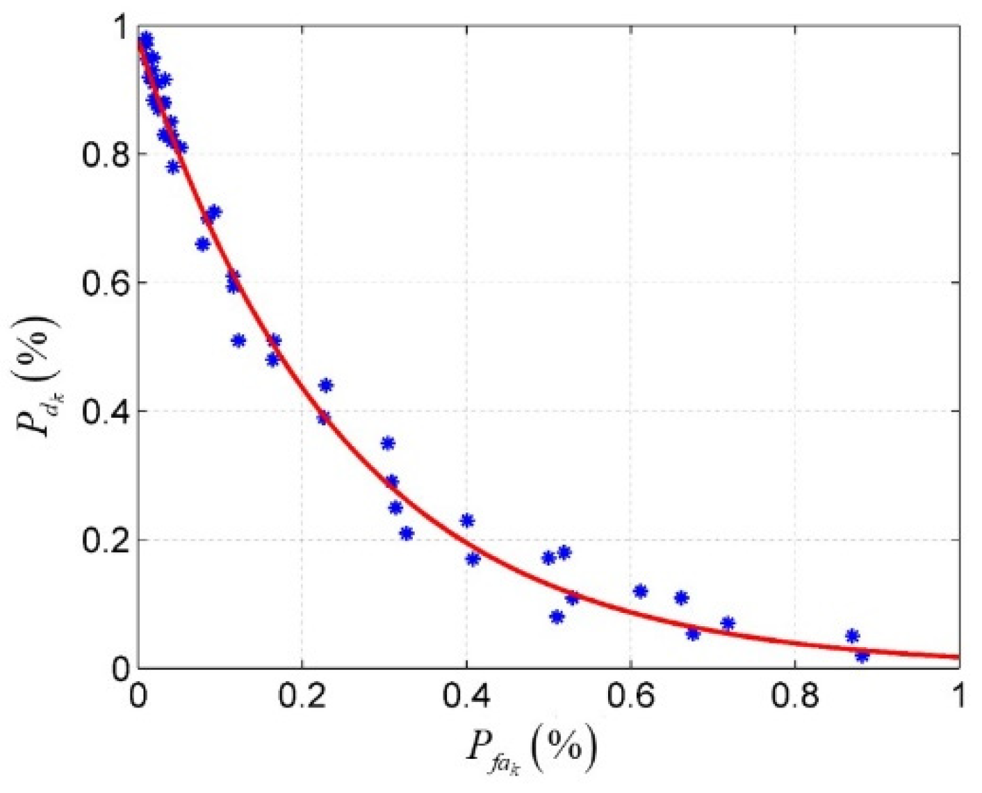
It can be found from
Table 1,
Table 2 and
Table 3 and
Figure 5 that under different system parameters, the changes of the relationship between the correct ranging probability
and the incorrect ranging probability
have a consistent trend. In other words, the influences of the three system parameters on the relationship between correct ranging probability
and incorrect ranging probability
are not significantly different. Based on this premise, in order to obtain more accurate and more general fitting result, we merge all data under different sequence length, pulse counting density and noise level. The curve fitting results are shown in
Figure 5.
In order to quantitatively describe the relationship between incorrect ranging probability
and correct ranging probability
, curve fitting is carried out on the discrete data in
Figure 4. The result of the curve fitting is shown in Equation (3)
The red solid line in
Figure 4 is the theoretical result of Equation (3), and the blue discrete point is composed of the simulation data in
Figure 3. It can be found that the fitting result has a high correlation with the simulation data. At the same time, we use Equation (3) to fit the simulation data under different system parameters in
Figure 3, and it can be found that the discrete points under three groups of simulation data are highly consistent with the theoretical results.
3.4. Correct Ranging Probability Model without Considering System Jitter
Under reasonable signal recognition threshold conditions, the correct ranging probability
of true random coding photon counting lidar can be written as
where
is the signal recognition threshold, and
is the number of correctly detected codes. It can be found from
Figure 2 that the correct ranging probability
of the true random coding photon counting lidar is composed of two parts: the correct ranging probability
that the detected signal ‘1’ codes number is equal to the signal recognition threshold (corresponding to the first item in Equation (4)) and the correct ranging probability that the detected signal ‘1’ codes number is higher than the signal recognition threshold (corresponding to the second item in Equation (4)). When the detected ‘1’ code number is equal to the signal recognition threshold, the probability of correctly extracting the target position can be expressed as Equation (2). Then, Equation (4) can be further written as
where
. The first term in Equation (5) is composed of two parts: the first part represents the probability of just detecting
k ‘1’ codes, and the second part represents the probability of correctly extracting the target position when the sequence detects
k ‘1’ codes. The product of the two parts is used to represent the probability that the target can be correctly extracted when the detected ‘1’ codes is equal to the signal identification threshold
k. The second term in Equation (5) is similar to the first term, which represents the probability that the sequence can correctly extract the target position when the detected ‘1’ codes number is higher than the signal recognition threshold. Eventually, based on Equation (5), we have established the correct ranging probability theoretical model of truly random coding photon counting lidar without considering system jitter.
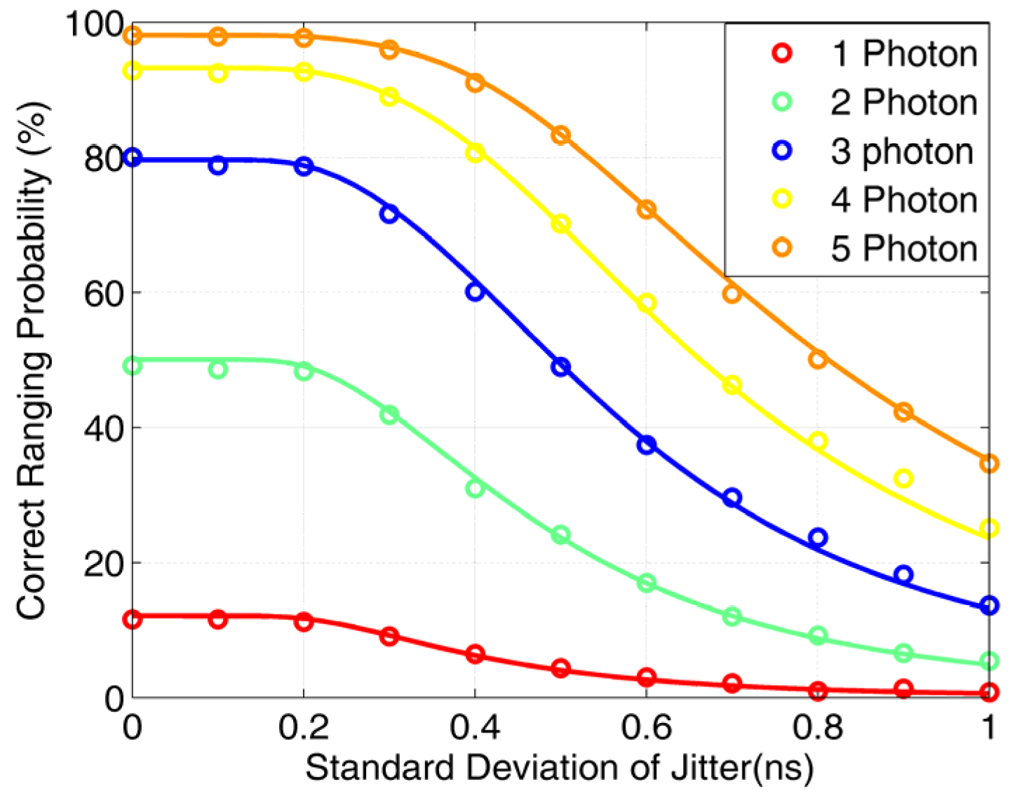
3.5. Correct Ranging Probability Model with Considering System Jitter
When there is a large jitter in the system, the impact of the jitter on the correct ranging probability should be considered. The reason why the jitter affects the correct ranging probability is that the true random coding photon counting lidar is based on the correlation operation to calculate the target distance. The jitter causes the ‘1’ code to shift forward or backward, resulting in matching error, thereby impacting the correct ranging probability. In the true random coding photon counting lidar system, the jitter is mainly composed of laser source, Gm-APD2 and TCSPC. In order to facilitate the analysis, the three jitter errors are considered comprehensively, and the FWHM (Full Width at Half Maxima) of the total jitter is .
When considering the effect of system jitter, the Equations (2)–(5) needs to be modified. Firstly, modify the incorrect ranging probability formula (Equation (2)). At this time, the incorrect ranging will include two parts: (1) the incorrect ranging caused by noise and (2) the incorrect ranging caused by the misplaced ‘1’ code due to the jitter.
is the FWHM of the system jitter, and the standard deviation of the jitter is
. Assuming that the jitter obeys the normal distribution of standard deviation
and mean value 0, then its probability distribution function is as follows:
When the jitter is considered, the probability that the ‘1’ code is not misaligned is
However, the probability of jitter dislocation of ‘1’ code is complex, which needs to be considered in two parts. Step 1: determine that the ‘1’ code can jitter up to a few pulse widths, in other words, there are several jitter positions for this code:
Step 2: determine the probability of jitter occurring at each position:
Therefore, when considering the system jitter, the incorrect ranging probability equation (Equation (2)) can be written as:
The correct ranging probability formula (Equation (5)) of reasonable threshold can be adjusted as:
Secondly, when considering the jitter, the correct ranging probability of the true random coding photon counting lidar can be modified as
5. Verify the Correct Ranging Probability Theoretical Model with Experiment
In order to further verify the theoretical model, we have built an experimental platform for a lidar system as shown in
Figure 9a. The main experimental parameters are shown in
Table 4. For the true random coding photon counting lidar, system jitter is mainly composed of three jitter sources: laser source, Gm-APD2 and TCSPC module. The jitter of Gm-APD2 can be obtained by datasheet, and the jitter of the laser source and TCSPC module can be measured by high bandwidth signal generator and high bandwidth linear detector. We adopt a simpler method to determine the system jitter. Instrument Response Function (IRF) summarizes overall characteristics of pulse width and system jitter. The FWHM (Full Width at Half Maxima) of the
, where
is pulse width and
is system jitter. For a fixed pulse width and system jitter, we can determine the system jitter by measuring the system response function. The IRF is obtained by measuring a flat target. Through a large number of statistical experiments, the IRF is shown in the
Figure 9b. Because the FWHM of IRF is 1.069 ns, pulse width is 1ns, so the FWHM of system jitter is 441 ps. Because the FWHM of system jitter is less than half of the minimum pulse width, the jitter has little effect on the correct ranging probability of our system. Therefore, the experiment verifies the correct ranging probability model without considering system jitter. The target with known distance is detected in the experiment. By comparing the distance detected by the experiment with the real distance, the correct detection probability of the system is determined.
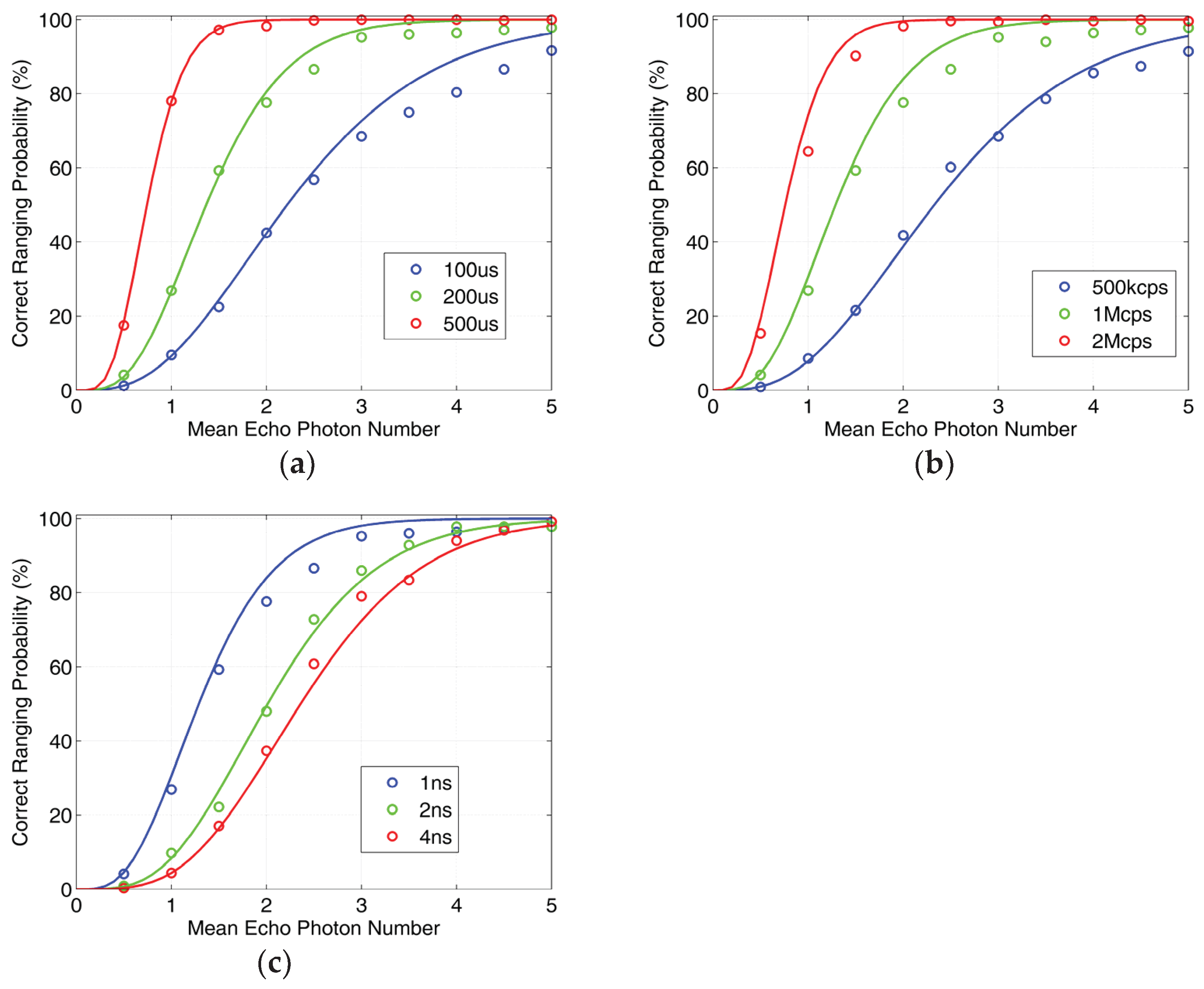
Figure 10a–c shows the variation of correct ranging probability with mean echo photon number under different sequence lengths, different pulse count density and different pulse width, respectively. The average detection probability of the emitted ’1’ code is calculated, and then the mean echo photon number of ’1’ codes is determined by the detection probability model of ‘1’ code. The circle represents the experimental result, and the solid line represents the theoretical result. Distinguish different system parameters with different colors. From
Figure 10 we can find that the experimental results are highly consistent with the theoretical results. Therefore, we have verified the correctness of the theoretical model through experiments. Based on the established theoretical model, the correct ranging probability can be effectively estimated according to the system parameters, which provides a reliable means for evaluating the detection performance of the system.
The echo intensity detected by photon counting lidar is in a photon level. Such high detection sensitivity makes it very sensitive to small changes in the system. Through our simulation and experiment, we can find that the change of one photon may make the detection probability change more than 50%. In the actual system, due to laser source instability, background noise changes, number of statistics, and other factors will cause changes in detection probability. As far as our experiment is concerned, there are two main causes of error: (1) the change of echo intensity caused by laser source instability and, (2) in the experiment, it is necessary to accurately adjust the echo photon to a certain intensity, such as 2 echo photons, which is very difficult for practical operation. Therefore, due to many inevitable errors in the experimental process, there are certain errors between the experimental and theoretical results. The simulation system can avoid these errors, so the simulation results are highly consistent with the theoretical results.

