Simulated Annealing Applied to HIO Method for Phase Retrieval


Abstract
:1. Introduction
2. Hybrid Input-Output (HIO) Algorithm
- (1)
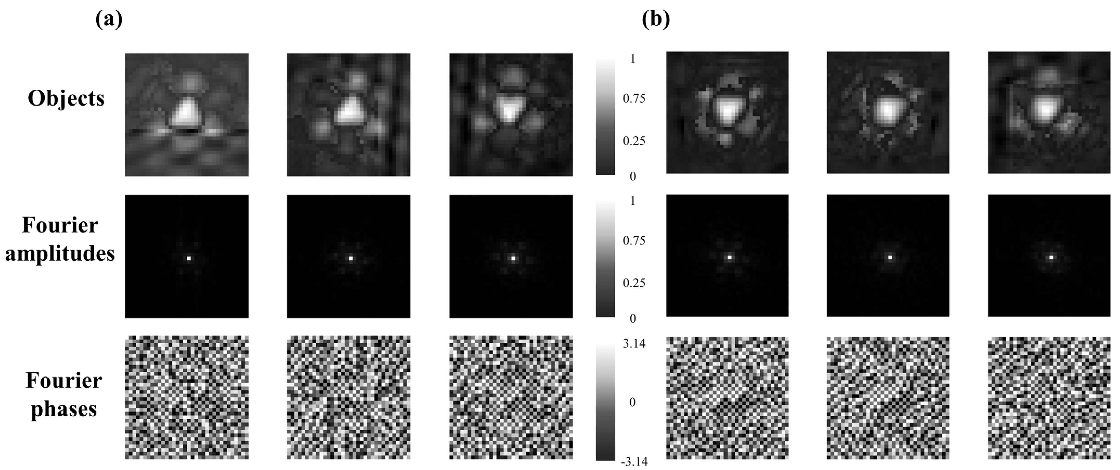
- Generate a random distribution in the object domain as an initial distribution. By performing Fourier transform on , a complex distribution is yielded in Fourier domain,where is the magnitude, and is the phase;
- (2)
- Replace the modulus with the measured magnitudes experimentally known as and keep its original phases to get a combinatorial , i.e.,
- (3)
- Generate an estimation in the object domain by inverse Fourier transformation as
- (4)
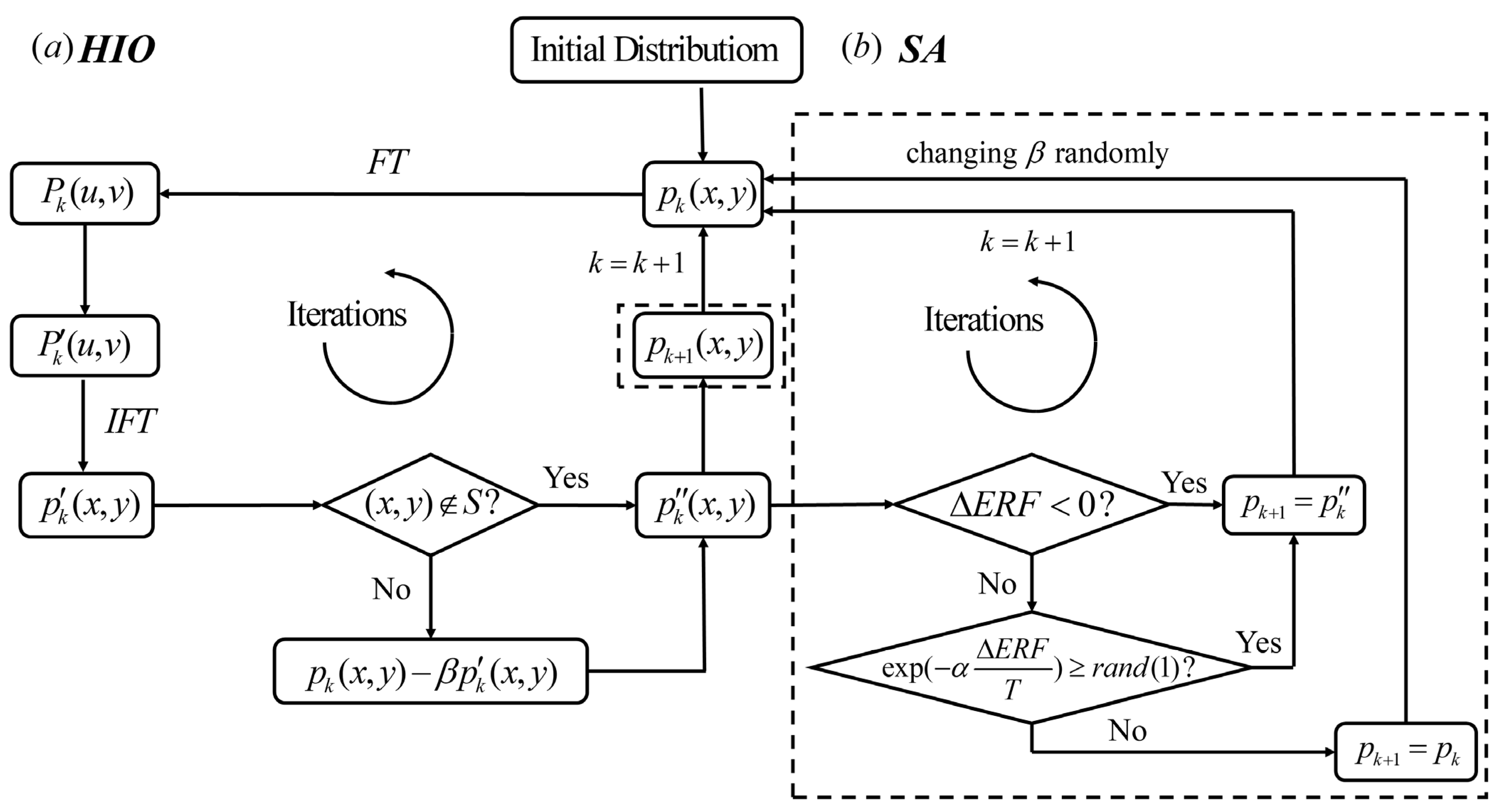
- For the iteration, i.e., the next iteration, the estimation of the object is determined aswhere is a constant and are the regions at which breaches the object-domain constraints, i.e., wherever is negative or it goes beyond the known area of the object [20]. A brief procedure of the HIO method is shown in Figure 1a.
3. Simulated Annealing Hybrid Input-Output
- (1)
- Start with an appropriate annealing temperature ;
- (2)
- Give a perturbation to get a random state close to the current one and calculate the cost function of the new one corresponding to the energy physically;
- (3)
- Accept the new state if where , and otherwise accept it on a probabilistic basis under the Metropolis criterion [25]. The annealing probability is given bywhere is the Boltzmann constant;
- (4)
- Decrease the temperature and start the next iteration from (2).
- (1)
- Generate a random initial distribution in the object domain and give an initial temperature and a value of . In our experiment, the initial temperature could be set as
- (2)
- Get the Fourier transformation just like Equation (1). Then substitute the modulus of , namely , with the measured data experimentally referred to as and keep its original phase angles to get integrated . Next, perform inverse Fourier transformation to acquire an estimate in the object domain, which is described in Equation (3);
- (3)
- For the iteration, i.e., the next iteration, calculate according to Equation (4) and then evaluate the errors of and respectively using an error function, i.e.,Furthermore, , regarded as an analogy with , is obtained by
- (4)
- Accept as at the beginning of the next iteration if or but it satisfieswhere is a random number generated by the computer, which satisfies uniform distribution between 0 and 1. In this way, we could simulate the annealing event according to probability because of . In other words, means accepting as according to the simulated annealing probability p. Otherwise, reject and make as to start the next iteration;
- (5)
- Change the value of β randomly between 0 and 1 for the next iteration. Moreover, decrease the temperature according to some criteria.
- (6)
- Lowering temperature too often and fast is not advised sometimes; that is to say, it is better to drop during every iteration, where is often greater than 1 and it could be set empirically;
- (7)
- The strategy of reducing is various and in this work, it decreases exponentially, i.e.,where γ is a constant between 0 and 1 and in this work it is set as 0.8.
| Algorithm 1: SAHIO (Simulated Annealing Hybrid Input-Output) |
| 1: Generate a random initial distribution and give the constraint regions ; |
| 2: Set the initial temperature and set ; |
| 3: Give the number of internal and external iterations, e.g., and ; |
| 4: Caculate according to Equation (8); |
| 5: for do |
| 6: for do |
| 7: set ; |
| 8: set , and ; |
| 9: caculate according to Equation (4); |
| 10: caculate according to Equation (8) and ; |
| 11: if then |
| 12: set ; |
| 13: else then |
| 14: generate a random number ; |
| 15: if then |
| 16: ; |
| 17: else then |
| 18: set and ; |
| 19: end if |
| 20: end if |
| 21: change the value of randomly; |
| 22: end for |
| 23: set ; |
| 24: end for |
4. Results
- (1)
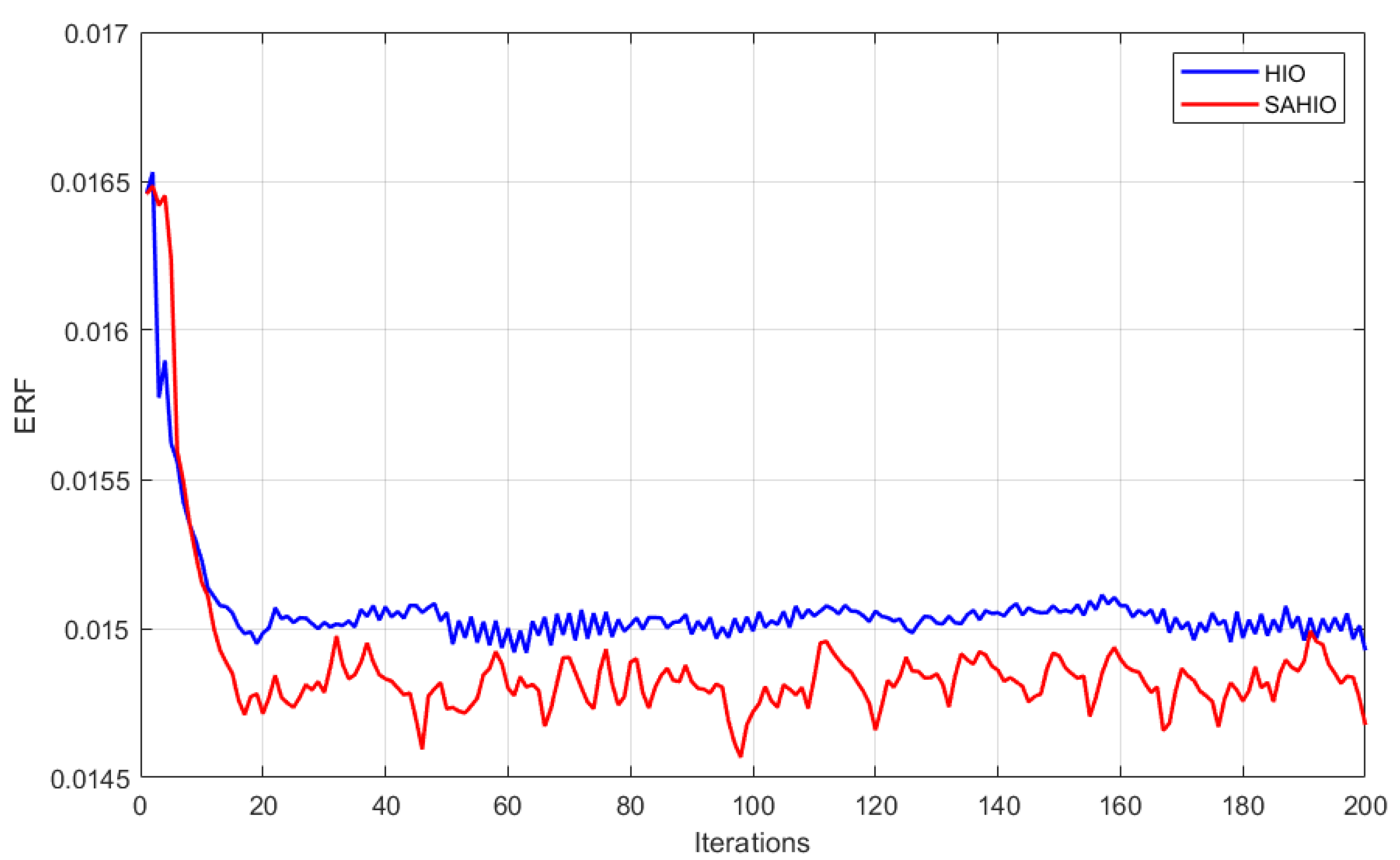
- Overall, the MSEs yielded by two algorithms decreased with increasing numbers of iterations with different speeds and results, which means that both methods have dissimilar degrees of the ability to reconstruct images.
- (2)
- Generally speaking, the SAHIO method declined faster than HIO. However, it is worth noting that in the early iterations, SAHIO, at a slight disadvantage for decreasing the MSE, showed a bit greater fluctuation owing to randomly changing. It was the random process of the exploration that delayed the time in the former steps but gave more chances to avoid the local minima in the latter stage.
- (3)
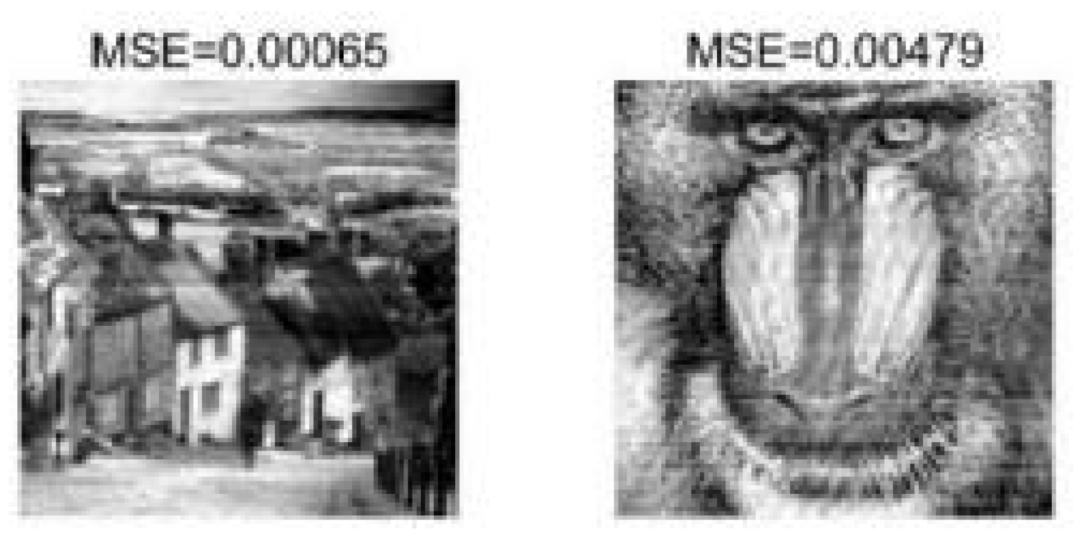
- At the end of 200 iterations, for 35 images the average MSE yielded by the SAHIO method converged at the lowest value, i.e., 0.00745, while the HIO method ended up with 0.01493; that is to say, the MSE generated by the SAHIO method was 50.12% smaller than the HIO method, demonstrating its strength of jumping out of the local minima and searching for the global optimum.
- (1)
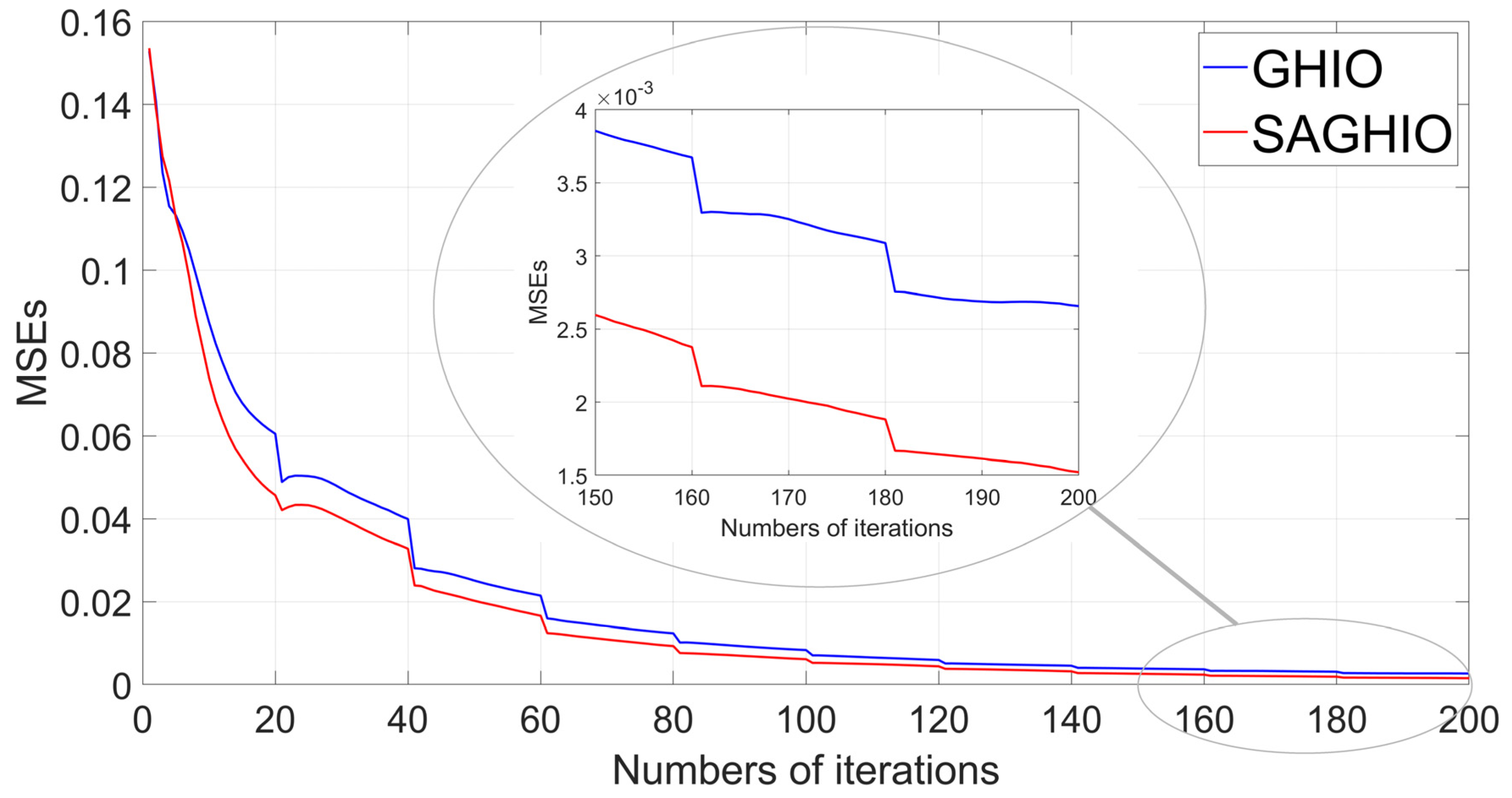
- The MSEs curve of SAGHIO converged faster than that of GHIO. In the beginning, SAGHIO performed a little worse; SAGHIO caught up quickly, but the speed advantage seemed less obvious with iterations going on;
- (2)
- At the end of 200 iterations, the MSEs of SAGHIO converged to a lower number, i.e., 0.00152, while GHIO was 0.00266. Due to the restriction of the axis scale, the difference of final MSEs between SAGHIO and GHIO was inapparent, but SAGHIO’s result was 42.857% better than GHIO’s indeed, which means SAGHIO could reconstruct images clearer in general.
5. Discussion
6. Conclusions
Author Contributions
Funding
Institutional Review Board Statement
Informed Consent Statement
Data Availability Statement
Conflicts of Interest
References
- Schnars, U.; Hartmann, H.J.; Jueptner, W.P. Digital recording and numerical reconstruction of holograms for nondestructive testing. In Proceedings of the SPIE 2545, Interferometry VII: Applications, San Diego, CA, USA, 9–14 July 1995; Volume 2545, p. 250. [Google Scholar]
- Petrov, N.V.; Gorodetsky, A.A.; Bespalov, V.G. Holography and phase retrieval in terahertz imaging. In Proceedings of the SPIE 8846, Terahertz Emitters, Receivers, and Applications IV, San Diego, CA, USA, 25–29 August 2013; Volume 8846, p. 88460S. [Google Scholar]
- Zhang, Y.; Pedrini, G.; Osten, W.; Tiziani, H.J. Whole optical wave field reconstruction from double or multi in-line holograms by phase retrieval algorithm. Opt. Express 2003, 11, 3234. [Google Scholar] [CrossRef] [PubMed]
- Dean, B.H.; Aronstein, D.L.; Smith, J.S.; Shiri, R.; Acton, D.S. Phase retrieval algorithm for JWST flight and testbed telescope. In Proceedings of the SPIE 6265, Space Telescopes and Instrumentation I: Optical, Infrared, and Millimeter, Bellingham, Orlando, FL, USA, 24–31 May 2006; Volume 6265, p. 626511. [Google Scholar]
- Baba, N.; Mutoh, K. Measurement of telescope aberrations through atmospheric turbulence by use of phase diversity. Appl. Opt. 2001, 40, 544. [Google Scholar] [CrossRef] [PubMed]
- Fienup, J.R. Space object imaging through the turbulent atmosphere. Opt. Eng. 1979, 18, 185529. [Google Scholar] [CrossRef]
- Harrison, R.W. Phase problem in crystallography. JOSA A 1993, 10, 1046. [Google Scholar] [CrossRef]
- Gerchberg, R.W. A practical algorithm for the determination of phase from image and diffraction plane pictures. Optik 1972, 35, 237. [Google Scholar]
- Fienup, J.R. Reconstruction of an object from the modulus of its Fourier transform. Opt. Lett. 1978, 3, 27. [Google Scholar] [CrossRef] [PubMed]
- Chen, C.C.; Miao, J.; Wang, C.W.; Lee, T.K. Application of optimization technique to noncrystalline X-ray diffraction microscopy: Guided hybrid input-output method. Phys. Rev. B 2007, 76, 064113. [Google Scholar] [CrossRef] [Green Version]
- Li, L.J.; Liu, T.F.; Sun, M.J. Phase retrieval utilizing particle swarm optimization. IEEE Photon. J. 2017, 10, 1. [Google Scholar] [CrossRef]
- Sun, M.J.; Zhang, J.M. Phase retrieval utilizing geometric average and stochastic perturbation. Opt. Lasers Eng. 2019, 120, 1. [Google Scholar] [CrossRef]
- Eldar, Y.C.; Kutyniok, G. Compressed Sensing: Theory and Applications; Cambridge University Press: Cambridge, UK, 2012. [Google Scholar]
- Moravec, M.L.; Romberg, J.K.; Baraniuk, R.G. Compressive phase retrieval. In Proceedings of the SPIE 6701, Wavelets XII, San Diego, CA, USA, 26–30 August 2007; Volume 6701, p. 670120. [Google Scholar]
- Faridian, A.; Hopp, D.; Pedrini, G.; Eigenthaler, U.; Hirscher, M.; Osten, W. Nanoscale imaging using deep ultraviolet digital holographic microscopy. Opt. Express 2010, 18, 14159. [Google Scholar] [CrossRef] [PubMed]
- Guo, C.; Li, Q.; Tan, J.; Liu, S.; Liu, Z. A method of solving tilt illumination for multiple distance phase retrieval. Opt. Lasers Eng. 2018, 106, 17. [Google Scholar] [CrossRef]
- Loewen, E.G.; Popov, E. Diffraction Gratings and Applications; CRC Press: Boca Raton, FL, USA, 1997. [Google Scholar]
- Jaganathan, K.; Eldar, Y.C.; Hassibi, B. Phase retrieval: An overview of recent developments. arXiv 2016, arXiv:1510.077132015. [Google Scholar]
- Kirkpatrick, S.; Gelatt, C.D.; Vecchi, M.P. Optimization by simulated annealing. Science 1983, 220, 671. [Google Scholar] [CrossRef] [PubMed]
- Fienup, J.R. Phase retrieval algorithms: A comparison. Appl Opt. 1982, 21, 2758. [Google Scholar] [CrossRef] [PubMed] [Green Version]
- Nieto-Vesperinas, M.; Mendez, J.A. Phase retrieval by Monte Carlo methods. Opt. Commun. 1986, 59, 249. [Google Scholar] [CrossRef] [Green Version]
- Nieto-Vesperinas, M.; Navarro, R.; Fuentes, F.J. Performance of a simulated-annealing algorithm for phase retrieval. JOSA A 1988, 5, 30. [Google Scholar] [CrossRef] [Green Version]
- Kim, M.S.; Guest, C.C. Simulated annealing algorithm for binary phase only filters in pattern classification. Appl. Opt. 1990, 29, 1203. [Google Scholar] [CrossRef] [PubMed]
- Van Laarhoven, P.J.M.; Aarts, E.H.L. Simulated Annealing, Simulated Annealing: Theory and Applications; Springer: Dordrecht, The Netherlands, 1987. [Google Scholar]
- Metropolis, N.; Rosenbluth, A.W.; Rosenbluth, M.N.; Teller, A.H.; Teller, E. Equation of State Calculations by Fast Computing Machines. J. Chem. Phys. 1953, 21, 1087. [Google Scholar] [CrossRef] [Green Version]


Publisher’s Note: MDPI stays neutral with regard to jurisdictional claims in published maps and institutional affiliations. |
© 2021 by the authors. Licensee MDPI, Basel, Switzerland. This article is an open access article distributed under the terms and conditions of the Creative Commons Attribution (CC BY) license (https://creativecommons.org/licenses/by/4.0/).
Share and Cite
Zhang, Y.; Sun, M. Simulated Annealing Applied to HIO Method for Phase Retrieval. Photonics 2021, 8, 541. https://doi.org/10.3390/photonics8120541
Zhang Y, Sun M. Simulated Annealing Applied to HIO Method for Phase Retrieval. Photonics. 2021; 8(12):541. https://doi.org/10.3390/photonics8120541
Chicago/Turabian StyleZhang, Yicheng, and Mingjie Sun. 2021. "Simulated Annealing Applied to HIO Method for Phase Retrieval" Photonics 8, no. 12: 541. https://doi.org/10.3390/photonics8120541
APA StyleZhang, Y., & Sun, M. (2021). Simulated Annealing Applied to HIO Method for Phase Retrieval. Photonics, 8(12), 541. https://doi.org/10.3390/photonics8120541