Chromatic Dispersion Equalization FIR Digital Filter for Coherent Receiver

Abstract

Chromatic dispersion equalization (CDE) in coherent optical communication systems is extremely critical for subsequent digital signal processing (such as frequency offset estimation and carrier phase recovery). Various methods mentioned in the published literature are not satisfactory when the signal bandwidth is limited. This paper proposes a way of using singular value decomposition least square (SVDLS) to obtain the optimal tap weight of the CDE filter and a method to introduce the adaptive mutation particle swarm optimizer (AMPSO) algorithm into the CDE. We show that the two proposed approaches are based on the best approximation of the frequency domain response of the designed and ideal CDE filter. Compared with the traditional CDE method, which needs to be implemented in the full frequency band, the two methods can be implemented in the narrow frequency band. The simulation shows that the effective bandwidth of the baseband signal is limited by squared-root-raised-cosine (SRRC) pulse shaping with a roll-off factor of 0.25 in different modulation formats (DP-QPSK, DP-16 QAM, DP-64 QAM) when the number of taps of the filter is 131, which is 37.5% less than the full frequency band. The designed filter is superior to the existing filter in terms of filtering effect and implementation complexity.

1. Introduction

With the expansion of the 5G network construction scale and the innovative development of the industrial internet, the construction of the optical network is marching towards higher speed, large capacities, and long distances [1]. In the case of long-distance transmission systems, such as submarine optical cables, the accumulated transmission loss, nonlinear effects, and chromatic dispersion (CD) cause the deterioration of high-speed optical fiber system performance. The erbium-doped fiber amplifier (EDFA) is introduced to overcome transmission loss and the optical power is monitored to suppress the nonlinear effect. The CD has become the major obstacle to upgrading the optical network industry [2]. In a wide-band system (64 GBaud or higher), the inter-symbol interference (ISI) caused by CD extends over more than 150 symbols after 250 km of fiber transmission and preclude long-distance transmission without proper chromatic dispersion equalization (CDE) [3].

CD has been effectively compensated in the optical and electrical domains. In the optical domain, equipment with large negative CD is mainly used for compensation [4]. With the development of high-speed analog-to-digital (ADC) converter and coherent detection techniques, digital coherent receivers can compensate for large amounts of accumulated CD in the electrical domain at negligible cost through digital signal processing (DSP) methods [5,6,7]. A series of strategies for achieving CDE in the time domain (TD) and frequency domain (FD) has been verified in commercial DSP [8,9,10,11,12,13,14,15].

Frequency domain chromatic dispersion equalization (FD-CDE) involves overlap-save (OLA) or overlap-add zero padding (OLA-ZP) methods, and the complexity evolves with ${\mathrm{N}}_{\mathrm{FFT}}{\log }_2\left({\mathrm{N}}_{\mathrm{FFT}}\right)$, where ${\mathrm{N}}_{\mathrm{FFT}}$ is the block size of fast Fourier transform (FFT). The complexity of time-domain chromatic dispersion equalization (TD-CDE) is ${\mathrm{N}}^2$, where N is a variable related to the CD to be equalized. The overall performance of FD-CDE is better than that of TD-CDE in long-distance fiber links [16], so it’s considered to be the most suitable choice for commercial coherent receivers [17]. However, FD-CDE requires time-frequency conversion of the input sequence, which may cause time aliasing. In addition, poor interaction with nonlinear components and other TD modules limits the reduction of energy consumption [18]. At present, the CDE module consumes a lot of energy in DSP, which is an important factor in restricting compact transceiver’s upgrading. In the model prediction of 2400 km 100 Gbit/s DP-QPSK coherent optical communication system compensating 30 ps mean differential group delay (DGD), the CDE module accounts for 36% of the receiver DSP energy consumption [19]. So, to reduce the hardware requirements and improve the coherent receiver efficiency, it’s necessary to reduce the complexity associated with CDE.

Since the entire equalization process of TD-CDE is carried out in TD, which avoids the possible problems in FD-CDE. Savory proposed the FIR CDE filter in a closed-form in the TD [20]. Four main drawbacks need to be revisited as (I) the filter needs to equalize the accumulative CD in the full frequency band, (II) the performance of the filter will deteriorate if the length of the filter is increased, (III) the length of the filter is positively correlated with the CD to be compensated, and (IV) the compensation quality is poor under the high-order modulation format. Driven by this motivation, some FIR filter-based CDE methods have been proposed to reduce complexity [21,22]. From an implementation point of view, the main challenge to reduce the power consumption of the CDE module is the length of the filter. Eghbali uses the energy convex minimization method of the complex error between the frequency response of the actual CDE filter and the ideal CDE filter, and the FIR filter is designed in the least square (LS) sense to compensate the accumulative CD only in the effective frequency band [23]. Even though the band-limited CDE significantly shortens the length of the filter compared with [20], the total amount of calculation derived from it is very high, and the proof is given in Section 2. Despite many drawbacks, the development prospects in this field are still promising.

In this paper, we propose two new methods for constructing FIR filters to compensate accumulative CD, and both ways seek the optimal weights as filter tap coefficients. In our work, we first build a set of FIR filters. When the FD response of the constructed FIR filter is infinitely close to the ideal FD-CDE filter, the filtering performance of the former is also optimal. One of the methods is based on the singular value decomposition least squares (SVDLS) to obtain the optimal weight. This method uses the relationship between the two FD responses to construct a linear overdetermined equation and uses the SVDLS method to find the optimal solution as the tap coefficient of the filter. Another way is to use the adaptive mutation particle swarm optimization (AMPSO) algorithm to quickly find the optimal weights through iterative optimization calculations so that the two FD responses reach the best approximation. The simulation results show that both types of new FIR filters can effectively implement CDE. The proposed method is compared with the standard TD-CDE, and the results show that the proposed filter performs better and makes up for the four main drawbacks mentioned above. Compared with FD-CDE, the proposed filter requires fewer taps under the same BER.

The rest of this paper is organized as follows. In Section 2, the existing methods of FD-CDE and TD-CDE are briefly introduced, the FIR filter FD response function in the LS sense is derived, and proves that the way in [23] has redundant calculations. The theoretical formulas behind the two types of FIR filters are given, and the complexity is analyzed. In Section 3, numerical simulations are carried out, and the proposed methods are compared with TD-CDE and FD-CDE in the full frequency band and the narrow frequency band. 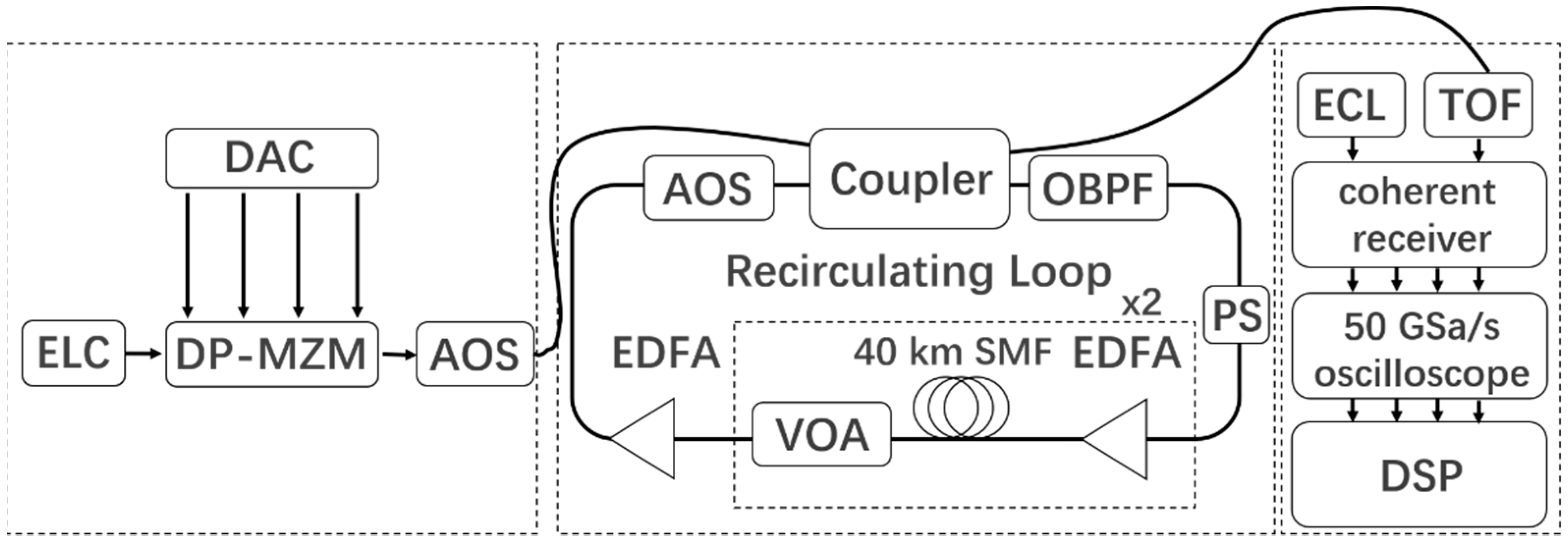In Section 4, we analyzed the performance of the two proposed CDE FIR filters and TD-CDE filters on the experimental platform of 28 GBaud PDM-16 QAM. In Section 5, the application scenarios of the two proposed CDE schemes are discussed. Finally, Section 6 gives the conclusion.

2. Principle

The following partial differential equation can model CD’s influence on the signal envelope $U(z,\tau )$ to simplify the structure of the coherent receiver, which is also the basis of all CDE algorithms [24].

$$\frac{\partial U(z,\tau )}{\partial z}=\mathrm{j}\frac{D{\lambda }^2}{4\pi c}\frac{{\partial }^{2}U(z,\tau )}{\partial {\tau }^2}$$

(1)

where $z$ is the propagation distance, $\tau$ is the normalized time parameter, $D$, $\lambda$, $c$ are the CD coefficient, wavelength, and the speed of light. Taking the FFT of Equation (1) to acquire the FD transfer function $G(z,w)$ given by,

$$G(z,w)=\exp \left(-\mathrm{j}\frac{D{\lambda }^2}{4\pi c}{\omega }^2\right)$$

(2)

here, $\omega$ represents the digital frequency with any frequency component. Invert the sign of the $D$ in Equation (2), and the CD can be compensated by an all-pass filter to approximate the ideal frequency response as,

$$H\left(z,w\right)=1/G(z,\omega )=\exp \left(\mathrm{j}\frac{D{\lambda }^2}{4\pi c}{\omega }^2\right)$$

(3)

In addition to directly equalizing the CD in FD, the output can be obtained by convolution of the input sequence and the impulse response. Perform the inverse fast Fourier transform (IFFT) of Equation (3) to acquire the TD complex impulse response as,

$$h(k)=\sqrt{\frac{\mathrm{j}c{T}^2}{D{\lambda }^{2}z}}\exp \left(-\mathrm{j}\frac{\pi c{T}^2}{D{\lambda }^{2}z}{k}^2\right)-\lfloor \frac{N}{2}\rfloor ⩽k⩽\lfloor \frac{N}{2}\rfloor$$

(4)

where $\lfloor \rfloor$ represents the round-down operation, $T$ is the sampling interval, and $N$ is the length of the filter $h\left(k\right)$ given as,

$$N=2\lfloor \frac{\left|D\right|{\lambda }^{2}z}{2c{T}^2}\rfloor +1$$

(5)

2.1. Least-Squares FIR Filter

Consider a complex FIR digital filter of length is $N$ and its unit impulse response given by,

$$h(n)=h_{\mathrm{R}}(n)+\mathrm{j}{h}_1(n)-\frac{N-1}{2}\le n\le \frac{N-1}{2}$$

(6)

with a frequency response as,

$$H\left(e^{j\omega T}\right)={\displaystyle \sum _{n=-\frac{N-1}{2}}^{\frac{N-1}{2}}h}(n)e^{-jn\omega T}$$

(7)

Note that in the derivation of Equation (4), to avoid aliasing in the FD, TD truncation is required, limiting the number of taps. The band can be limited to Nyquist frequency $\omega =\pi /T$ to overcome this limitation, set the frequency range $\omega \in \left[{\omega }_1,{\omega }_2\right]$, and the square error ${\epsilon }^2$ between the desired and the actual response given by [25],

$$\begin{array}{ll}{\epsilon }^2& ={\displaystyle {\int }_{{\omega }_1}^{{\omega }_2}{\left|H(\omega )-H_d(\omega )\right|}^2}d\omega \\ & ={\displaystyle {\int }_{{\omega }_1}^{{\omega }_2}{\left(h^{T}e(\omega )-H_d(\omega )\right)}^{*}}\left(e^T(\omega )h-H_d(\omega )\right)d\omega \end{array}$$

(8)

Using gradient descent method to find the extreme value as,

$$\frac{d{\epsilon }^2}{dh}=0={\displaystyle {\int }_{{\omega }_1}^{{\omega }_2}{\left(h^{T}e(\omega )-H_d(\omega )\right)}^{*}}e(\omega )d\omega$$

(9)

hence, we have the tap coefficients T in an LS sense as,

$$\stackrel{\wedge }{h}={\displaystyle {\int }_{{\omega }_1}^{{\omega }_2}e}(\omega )H_d(\omega )d\omega$$

(10)

taking into account the n-order complex tap coefficients, Equation (10) can be equivalent to,

$$\stackrel{\wedge }{h}(n)=\frac{1}{2\pi }{\displaystyle {\int }_{{\mathrm{\Omega }}_1/T}^{{\mathrm{\Omega }}_2/T}{e}^{\left(j{\beta }_2{\omega }^{2}z/2\right)}}{e}^{jn\omega T}d(\omega T)$$

(11)

Simplify Equation (11) given by,

$$\begin{array}{ll}\stackrel{\wedge }{h}(n)& =\frac{T}{2\pi }{\displaystyle {\int }_{{\mathrm{\Omega }}_1/T}^{{\mathrm{\Omega }}_2/T}\exp }\left[\frac{j{\beta }_{2}z}{2}\left({\omega }^2+\frac{2n\omega T}{{\beta }_{2}z}\right)\right]d(\omega )\\ & =\frac{T}{2n}\exp \left(\frac{-j{n}^2{T}^2}{2{\beta }_{2}z}\right){\displaystyle {\int }_{{\mathrm{\Omega }}_1/T}^{{\mathrm{\Omega }}_2/T}\exp }\left[\frac{j{\beta }_{2}z}{2}{\left(\omega +\frac{nT}{{\beta }_{2}z}\right)}^2\right]d(\omega )\end{array}$$

(12)

taking $\frac{T}{2n}\exp \left(\frac{-j{n}^2{T}^2}{2{\beta }_{2}z}\right)$ as $A$, then Equation (12) is expressed as,

$$\begin{array}{ll}\stackrel{\wedge }{h}(n)& =A\cdot {\displaystyle {\int }_{{\mathrm{\Omega }}_1/T}^{{\mathrm{\Omega }}_2/T}\exp }\left[\frac{j{\beta }_{2}z}{2}{\left(\omega +\frac{nT}{{\beta }_{2}z}\right)}^2\right]d(\omega )\\ & =A\cdot {\displaystyle {\int }_{-{\mathrm{\Omega }}_1/T+\frac{nT}{{\beta }_{2}z}}^{{\mathrm{\Omega }}_2/T+\frac{nT}{{\beta }_{2}z}}\exp }\left[\frac{j{\beta }_{2}z}{2}{\left(\omega \right)}^2\right]d(\omega )\\ & =A\cdot \sqrt{\frac{2}{j{\beta }_{2}z}}\cdot {\displaystyle {\int }_{\sqrt{\frac{j{\beta }_{2}z}{2}}\left(-{\mathrm{\Omega }}_1/T+\frac{nT}{{\beta }_{2}z}\right)}^{\sqrt{\frac{j{\beta }_{2}z}{2}}\left({\mathrm{\Omega }}_2/T+\frac{nT}{{\beta }_{2}z}\right)}\exp }\left({\omega }^2\right)d(\omega )\end{array}$$

(13)

according to the Gaussian error function, which is defined as,

$$\mathrm{erf}(z)=\frac{2}{\sqrt{\pi }}{\displaystyle {\int }_0^z{e}^{-u^2}}du$$

(14)

Note that if $u$ is a complex variable, we obtain the error function in complex form as,

$$\mathrm{erf}(z)=-j\frac{2}{\sqrt{\pi }}{\displaystyle {\int }_0^z{e}^{{\left(ju\right)}^2}}d\left(ju\right)$$

(15)

Incorporating Equation (15) into Equation (13), we can obtain the optimal filter tap coefficient in the sense of LS as,

$$\stackrel{\wedge }{h}(n)=\frac{\exp \left(\frac{-j{n}^2{T}^2}{2{\beta }_{2}z}\right)}{2j\sqrt{2\pi {\beta }_{2}z}}(\mathrm{erf}\left[\sqrt{\frac{j{\beta }_{2}z}{2}}\left(\frac{nT}{{\beta }_{2}z}+{\mathrm{\Omega }}_2/T\right)\right]-\mathrm{erf}\left[\sqrt{\frac{j{\beta }_{2}z}{2}}\left(\frac{nT}{{\beta }_{2}z}-{\mathrm{\Omega }}_1/T\right)\right]$$

(16)

Comparing Equation (16) with Equation (9) in [23], it’s obvious that the computational complexity of the former is superior to the latter. Even though we reduce the total computation, which still involves solving the Gaussian error function, etc. We require further reduce the computation complexity.

2.2. Singular Value Decomposition Least-Squares FIR Filter

In this part, we adopt the idea of approximation to acquire the best match between the desired and actual response.

We note that for Equation (7), it can be rewritten as $H\left(e^{j\omega T}\right)=H\cdot {\mathrm{G}}^{\mathrm{T}}$, where $H$ and $\mathrm{G}$ are, respectively, given by,

$$\begin{array}{l}H=\left[h\left(-\frac{N-1}{2}\right),\dots ,h(0),\dots ,h\left(\frac{N-1}{2}\right)\right]\\ \mathrm{G}=\left[\exp \left(-\mathrm{j}\left(-\frac{N-1}{2}\right)\omega T\right),\dots ,\exp \left(-\mathrm{j}\left(\frac{N-1}{2}\right)\omega T\right)\right]\end{array}$$

(17)

Expressing $H$ and $\mathrm{G}$ with real and imaginary parts, then we can acquire as,

$$H\left(e^{j\omega T}\right)=\left({\mathrm{G}}_{\mathrm{R}}^{\mathrm{T}}{H}_{\mathrm{R}}+{\mathrm{G}}_{\mathrm{I}}^{\mathrm{T}}{H}_{\mathrm{I}}\right)+\mathrm{j}\left({\mathrm{G}}_{\mathrm{R}}^{\mathrm{T}}{H}_{\mathrm{I}}-{\mathrm{G}}_{\mathrm{I}}^{\mathrm{T}}{H}_{\mathrm{R}}\right)$$

(18)

Considering that the pulse shaping filter will limit the effective bandwidth of the signal $\omega =\mathrm{\Omega }/T$, set frequency range $\omega \in \left[{\omega }_1,{\omega }_2\right]$. Taking $K$ sampling points within the effective bandwidth, we can acquire as,

$$H\left(e^{j{\omega }_{\mathrm{i}}T}\right)=\left({\mathrm{G}}_{\mathrm{Ri}}^{\mathrm{T}}{H}_{\mathrm{R}}+{\mathrm{G}}_{\mathrm{Ii}}^{\mathrm{T}}{H}_{\mathrm{I}}\right)+\mathrm{j}\left({\mathrm{G}}_{\mathrm{Ri}}^{\mathrm{T}}{H}_{\mathrm{I}}-{\mathrm{G}}_{\mathrm{Ii}}^{\mathrm{T}}{H}_{\mathrm{R}}\right)i=1,\dots ,K$$

(19)

The FD response of the ideal filter is rewritten into the form of real and imaginary parts, and $K$ points are sampled in the same bandwidth, then it can be written as,

$$H\left(z,w_{\mathrm{i}}\right)=\cos \left(\mathrm{j}\frac{D{\lambda }^2}{4\pi c}{\omega }_{\mathrm{i}}{}^2\right)+\mathrm{j}\sin \left(\mathrm{j}\frac{D{\lambda }^2}{4\pi c}{\omega }_{\mathrm{i}}{}^2\right)i=1,\dots ,K$$

(20)

Combining Equation (19) and Equation (20), the real and imaginary parts of the FD response of the constructed FIR filter are, respectively, approximated to the real and imaginary part of the FD response of the ideal filter, and we can acquire as,

$$\begin{array}{l}\left({\mathrm{G}}_{\mathrm{Ri}}^{\mathrm{T}}{H}_{\mathrm{R}}+{\mathrm{G}}_{\mathrm{Ii}}^{\mathrm{T}}{H}_{\mathrm{I}}\right)=\cos \left(\mathrm{j}\frac{D{\lambda }^2}{4\pi c}{\omega }_{\mathrm{i}}{}^2\right)\\ \left({\mathrm{G}}_{\mathrm{Ri}}^{\mathrm{T}}{H}_{\mathrm{I}}-{\mathrm{G}}_{\mathrm{Ii}}^{\mathrm{T}}{H}_{\mathrm{R}}\right)=\sin \left(\mathrm{j}\frac{D{\lambda }^2}{4\pi c}{\omega }_{\mathrm{i}}{}^2\right)\end{array}i=1,\dots ,K$$

(21)

Equation (21) can be further simplified given by,

$$\left[\begin{array}{ll}{\mathrm{G}}_{\mathrm{Ri}}^{\mathrm{T}}\hfill & {\mathrm{G}}_{\mathrm{Ii}}^{\mathrm{T}}\hfill \\ -{\mathrm{G}}_{\mathrm{Ii}}^{\mathrm{T}}\hfill & {\mathrm{G}}_{\mathrm{Ri}}^{\mathrm{T}}\hfill \end{array}\right]\left[\begin{array}{c}{H}_{\mathrm{R}}\\ H_{\mathrm{I}}\end{array}\right]=\left[\begin{array}{c}\cos \left(\mathrm{j}\frac{D{\lambda }^2}{4\pi c}{\omega }_{\mathrm{i}}{}^2\right)\\ \sin \left(\mathrm{j}\frac{D{\lambda }^2}{4\pi c}{\omega }_{\mathrm{i}}{}^2\right)\end{array}\right]i=1,\dots ,K$$

(22)

Equation (22) is the constructed overdetermined equations given by,

$$Ax=bA\in R^{2m\ast 2n},x\in R^{2n},b\in R^{2m}$$

(23)

For the overdetermined problems and generally non-uniform equations, the equations have no solution. Then turn to solve the LS problem, that is to minimize ${\Vert Ax=b\Vert }_2^2$, the LS solution can be obtained as,

$$x={\left(A^{T}A\right)}^{-1}{A}^{T}b$$

(24)

There are two main problems in the solution method mentioned above, such as (I) involves the inversion operation of $2m\ast 2n$-dimensional matrix, which requires a large amount of calculation, (II) $A^{T}A$ may be irreversible. To overcome the above limitations, we propose a method based on SVDLS. In contrast with eigenvalue decomposition, which can only be applied to square matrices, any matrix $A\in R^{m\ast n}$ can be SVD to,

$$A_{\mathrm{svd}}=\left[U\right]\left[S\right]\left[V^T\right]U\in R^{m*m},S\in R^{m*n},V\in R^{n*n}$$

(25)

where $U$ and $V$ are orthogonal matrices, $S={\left[\mathrm{\Sigma }0\right]}^{{}^T}$, $\mathrm{\Sigma }$ is a diagonal matrix, and it’s the value of matrix $A$, which is completely determined by $A$ and independent of $U$$V$. Next, we reconsider the LS problem given by,

$$\Vert Ax=b{\Vert }_2^2=\Vert U\left[\begin{array}{c}\mathrm{\Sigma }\\ 0\end{array}\right]V^{T}x-b\Vert =\Vert \left[\begin{array}{c}\mathrm{\Sigma }\\ 0\end{array}\right]V^{T}x-Ub\Vert$$

(26)

where $U$ can be disassembled into $\left[U_n,U_{m-n}\right]$, that $U_n$ is the first $n$-column matrix of $U$, and then obtained as,

$$\begin{array}{ll}\Vert Ax=b{\Vert }_2^2& =\Vert \left[\begin{array}{c}\mathrm{\Sigma }\\ 0\end{array}\right]V^{T}x-{\left[U_n,U_{m-n}\right]}^{T}b\Vert \\ & =\Vert \left[\begin{array}{c}\mathrm{\Sigma }{V}^{T}x-U_n^{T}b\\ -U_{m-n}^{T}b\end{array}\right]\Vert \\ & =\Vert \mathrm{\Sigma }{V}^{T}x-U_n^{T}b\Vert +\Vert U_{m-n}^{T}b\Vert \ge \Vert U_{m-n}^{T}b\Vert \end{array}$$

(27)

It’s obvious that when ${\Vert Ax=b\Vert }_2^2$ takes the minimum value, if and only if $\Vert \mathrm{\Sigma }{V}^{T}x-U_n^{T}b\Vert =0$. The SVDLS solution can be obtained as,

$$x_{SVDLS}={\left(\mathrm{\Sigma }{V}^T\right)}^{-1}{U}_n^{T}b=V{\mathrm{\Sigma }}^{-1}{U}_n^{T}b$$

(28)

According to the SVDLS method, there must be a solution. Both $U$ and $V$ are orthogonal matrices, so the transposed matrix is equal to the inverse matrix. $\mathrm{\Sigma }$ is a diagonal matrix, and the singular values in the matrix in order from large to small, decay rate is particularly fast. The sum of the top 10% of the singular values usually accounts for more than 99% of the total, so we can further reduce the size of the matrix by discarding all the singular values below a certain threshold.

2.3. Adaptive Mutation Particle Swarm Optimizer FIR Filter

In the problem of parameter fitting, the LS method is often used, but when the function parameters are too large, the iteration times will be too many, and it’s easy to fill into the local optimal solution. Therefore, modern optimization algorithms are used in parameter fitting, commonly used genetic algorithms (GA) and particle swarm optimization (PSO) algorithms. PSO converges better than GA, no coding and crossover operation are needed, and that’s easier to implement with fewer parameters.

2.3.1. Traditional Particle Swarm Optimization Algorithm

The traditional PSO algorithm is derived from the study of bird predation behavior and finds the optimal solution through cooperation and information sharing among individuals in the group [26]. All particles are a possible solution in search space. Each particle performs an iterative update of its speed and position according to the individual extreme, global extreme, and its own experience. The position is evaluated by the fitness function of the algorithm. Each dimension of the particle has the limit of allowable value, and the particle that satisfies the constraint condition is the effective particle. Some parameter definitions in the PSO algorithm are list in

Table 1. Parameter definition in PSO algorithm.

Variable	Value	Comment
$X$	$\left(X_1,X_2,\dots ,X_n\right)$	The total group containing $n$ subgroups
$X_i$	$\left(x_{i1},x_{i2},\dots ,x_{iD}\right)$	The position vector of the $i$ particle
$V_i$	$\left(v_{i1},v_{i2},\dots ,v_{iD}\right)$	The velocity vector of the $i$ particle
$P_i^k$	$\left(P_{i1}^k,P_{i2}^k,\dots ,P_{iD}^k\right)$	Particle’s extremum of the $k$ iteration
$P_g^k$	$\left(P_{g1}^k,P_{g2}^k,\dots ,P_{gD}^k\right)$	Global extremum of the $k$ iteration

.

The iterative update equation of the particle’s position and velocity given by [27,28]

$$\begin{array}{c}{V}_{id}^{k+1}=w{V}_{id}^k+c_1{r}_1\left(P_{id}^k-X_{id}^k\right)+c_2{r}_2\left(P_{gd}^k-X_{id}^k\right)d=1,2,\cdots ,D\\ X_{id}{}^{k+1}=X_{id}^k+V_{id}^{k+1}i=1,2,\cdots ,n\end{array}$$

(29)

where $w$ denotes the inertia weight; $c_1$ and $c_2$ denote the learning factors; $r_1$ and $r_2$ denote the random numbers distributed between 0 and 1. Traditional PSO algorithms often fall into the situation of slow convergence speed, premature convergence, and weak local searchability in the later search stage, so it isn’t easy to obtain the global optimal solution.

2.3.2. Adaptive Mutation Particle Swarm Optimization Algorithm

In this paper, by improving the PSO algorithm, a new PSO algorithm is proposed to overcome the shortcomings of the traditional PSO algorithm. The improvement is embodied in two aspects: (I) adjust inertia weight based on particle fitness to improve the convergence speed of the algorithm, (II) use GA to introduce mutation operations to increase the activity of the population and avoid the algorithm falling into local convergence.

• Inertia weight optimization

Different particle search capabilities are need in the process of population exploration. Traditional PSO algorithm usually adopts linear decreasing weight method given by,

$$w=w_{\max }-\frac{k\left(w_{\max }-w_{\min }\right)}{{\mathrm{m}}_{gen}}k=1,2,\cdots ,{\mathrm{m}}_{gen}$$

(30)

where $w$ is the weight of inertia, $k$ is the current iteration number, and ${\mathrm{m}}_{gen}$ is the maximum possible iteration number. In the process of optimization, the distance between the particle and the optimal solution is different. Only the search time is taken into account to adjust the weight without involving the state of the particle itself, which affects the accuracy of the optimal solution. Therefore, we add the fitness of the particle to the weight adjustment strategy and defined as,

$$\begin{array}{c}{w}_{\mathrm{p}}=w_{\max }-(w_{\max }-w_{\min }){(\mathrm{k}/{\mathrm{m}}_{gen})}^2\\ w=w_{\min }+({\mathrm{n}}_{\mathrm{sum}}^{\mathrm{k}}-{\mathrm{n}}_{\mathrm{i}}^{\mathrm{k}})(w_{\mathrm{p}}-w_{\min })/({\mathrm{n}}_{\mathrm{sum}}^{\mathrm{k}}-{\mathrm{n}}_{\mathrm{vag}}^{\mathrm{k}})\end{array}$$

(31)

Here, $w_{\max }$ and $w_{\min }$ are the maximum and minimum of the inertia weight, ${\mathrm{n}}_{\mathrm{sum}}^{\mathrm{k}}$ and ${\mathrm{n}}_{\mathrm{vag}}^{\mathrm{k}}$ are the sum and average of the fitness of the particles in the $\mathrm{k}$ iteration of the population, ${\mathrm{n}}_{\mathrm{i}}^{\mathrm{k}}$ is the fitness of the $\mathrm{i}$ particle at the $\mathrm{k}$ iteration of the population. From the global exploration process perspective, the particle swarm needs to fly in a large range in the early stage, and the $w$ is larger. As the optimal solution range shrinks, the corresponding $w$ is smaller to guarantee accuracy. From the perspective of local search, particles with better fitness require weaker exploratory power than those with worse fitness and require small $w$.

Compared with the traditional methods that adopt the strategy of fixed weight or change the inertial weights according to the exploration time, we proposed a method of dynamically adjusting the inertial weights $w$ based on the particle fitness, it can not only take into account the global space exploration capability and the accuracy of the local searching solution, but also avoid the violent oscillation of particles near the optimal solution, so it has stronger convergence ability and searching efficiency.

• Introduce mutation strategy

The mutation strategy of GA is introduced into the particle search process, which can constitute interference factors to restrain the traditional method from falling into premature and increase the diversity of the later population, increase the scale of the particle in the search space, and improve the ability of the algorithm to jump out of local optimum. On the one hand, the mutation is introduced in the iterative update of the particle position vector, and Equation (32) is replaced with Equation (29) as,

$$X_{id}{}^{k+1}=X_{id}^k+V_{id}^{k+1}+\mathrm{A}\cdot ({\mathrm{m}}_{gen}-k)(X_{\max }+rand(1,D)(X_{\max }-X_{\min }))/{\mathrm{m}}_{gen}$$

(32)

where $D$ is the dimension of the particle, $X_{\max }$ and $X_{\min }$ are the upper and lower boundaries of the particle position vector, and $\mathrm{A}$ is the constant. On the other hand, the Gaussian probability distribution is used to perform a positional variation on the relative dimensions of a certain probability particle, and the mutation proceeds given by,

$$X_{id}{}^{k+1}=X_{id}^k\cdot (1+randn)$$

(33)

The introduction of Gaussian mutation may allow particles to escape the local minimum and enhance the population’s vitality.

2.3.3. FIR Filter Design Based on an Improved Algorithm

Applying the AMPSO algorithm to the FIR filter design, this study uses an overdetermined system of linear equations (given by Equation (23)) as the fitness function. The flow diagram of the design method is shown in Figure 1, with each step is as follows.

Step 1: data preprocessing. Calculate the fitness function Equation (23), and the solution process is the same as the previous chapter.

Step 2: parameter initialization. The maximum number of iterations, population size, inertia weight, learning factor. Coding for all particles and random initialization of position and velocity.

Step 3: update the particle status. Calculate the fitness value of the particle, adjust the particle inertia weight according to Equation (31), the position vector and velocity vector of the particle is updated by Equations (29) and (32), and perform boundary condition processing.

Step 4: fitness assessment. Recalculate the fitness of the current particle, update the individual extreme value $P_i^k$ of all particles, and store the optimal individual in the global optimal $P_g^k$.

Step 5: termination of condition review. If the current global optimum satisfies the accuracy or reaches the maximum number of iterations, jump out of the iteration and go to step 8. Otherwise, it moves to the next step.

Step 6: mutation. Perform mutation operation on the position vector of the particle. If the fitness after mutation is better, keep it, otherwise cancel the current mutation operation.

Step 7: repeat. Update the number of iterations and return to step 3.

Step 8: output the results. The global optimal particles are used as the coefficients of the FIR filter given by,

$$x_{AMPSO}=P_g^k$$

(34)

2.4. Implementation Complexity

Usually, the complexity we discuss includes design complexity and implementation complexity. Design complexity refers to the amount of calculation that needs to be implemented to obtain the weight of the digital filter, and implementation complexity refers to the amount of work required for the digital filter to achieve equalization. In coherent optical communication, the weight of the CDE filter needn’t be changed frequently, and the main workload comes from the implementation process of the CDE, so we mainly discuss the implementation complexity.

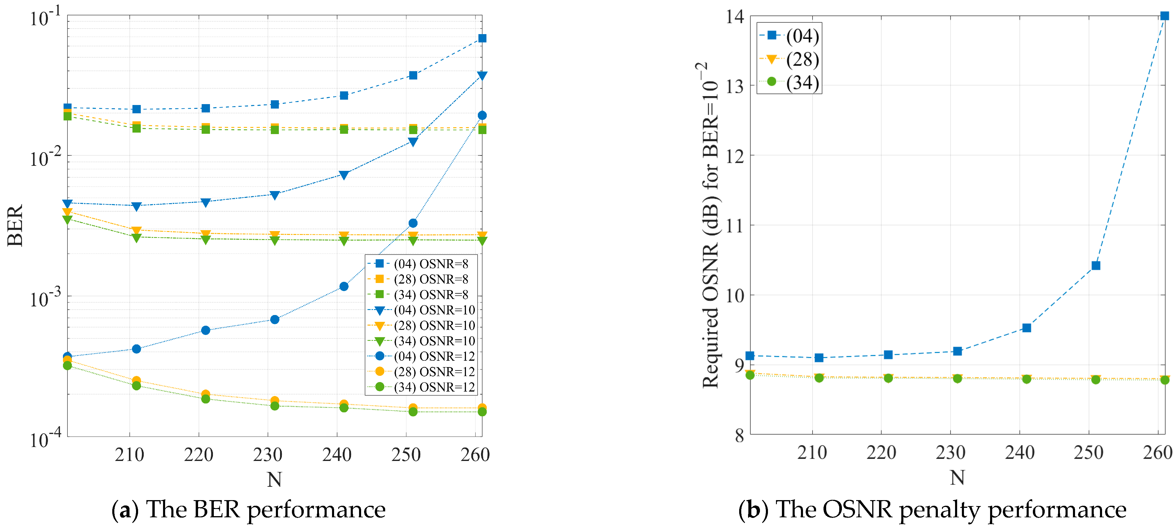
In TD-CDE, the implementation complexity of the filter is $N^2$, where $N$ is the number of FIR filter taps, and $N$ is positively correlated with the accumulated CD in the fiber channel. Therefore, for long-haul fiber links, TD-CDE requires more computing resources. In the numerical simulation of the third chapter, we have analyzed that compared with the filter in (4), the filter (28) and (34) that we designed on the finite frequency band $\mathrm{\Omega }=\pi \left(\left(1+\rho \right)/L\right)$ achieve the same BER performance, the number of filter taps $N$ required is significantly reduced. From the perspective of the amount of calculation, the implementation complexity of the filter we proposed will be lower than the filter in (3). So we can further infer that as the transmission distance increases, the difference in the number of taps between the filter we designed and the filter in (3) will gradually increase, and the reduction of the filter length is always beneficial.

3. Simulation and Discussion

3.1. Simulation Configuration

To verify the effectiveness of the two proposed FIR filter schemes in CDE, we use Optisystem 15 to build a coherent optical communication system numerical simulation platform, and the DSP module is implemented in MATLAB. The structural block diagram of the system is depicted in Figure 1.

The system adopts a square root raised cosine (SRRC) pulse signal generator at the transmitter and SRRC filter at the receiver for matched filtering. The SRRC filter can solve the problem of limited bandwidth while avoiding the introduction of inter-symbol interference. The stopband boundary of these filters is,

$$\mathrm{\Omega }=\pi \frac{1+\rho }{L}$$

(35)

here $\rho$ is the roll-off factor, and $L$ is the oversampling rate, usually an integer factor. The SRRC filter is used as [23],

$$g_{TX}(t)=g_{RX}(t)=\frac{\sin \left(\frac{\pi t}{T}(1-\rho )\right)+\frac{4\rho t}{T}\cos \left(\frac{\pi t}{T}(1+\rho )\right)}{\frac{\pi t}{T}\left(1-{\left(\frac{4\rho t}{T}\right)}^2\right)}$$

(36)

when $\rho =1$ or $0<\rho <1$, the CDE is in the full bandwidth or the bandwidth limited. ADC samples the sequence at twice the symbol rate before sending the sequence to the MATLAB component to complete DSP.

Table 2. System simulation parameter.

Parameter	Value	Parameter	Value
Wavelength	1550 nm	Chromatic dispersion coefficient	16.75 ps/nm/km
Sequence length	131,072	Group velocity dispersion coefficient	0.2 ps/km
Symbol rate	28/64 GBaud	Laser line width	0.1 MHz
Modulation format	DP-QPSK/16 QAM/64 QAM	Attenuation coefficient	0.2 db/km
Roll-off factor	1/0.25	Signal power	10 dbm
Population size	1000	Maximum number of iterations	1200

shows the system parameters.

3.2. Compared with the TD-CDE

We will compare the standard TD-CDE filter, such as Equation (4), with the two proposed filters, such as Equations (28) and (34). The number of sample points $K$ in SVDLS and AMPSO algorithms is set to three times the length of the filter.

3.2.1. Full Bandwidth Case

In this chapter, we compare filters using $\rho =1,L=2$, so it needs to compensate for CD in the full frequency bandwidth of $\mathrm{\Omega }\in [-\pi ,\pi ]$.

• Required OSNR versus CD at the same filter lengths.

To visually compare the performance of the three CDE filters under different transmission distances, set the system BER to 10⁻², and the relationship between CD and the required OSNR as shown in Figure 2.

As can be seen from Figure 2 that the OSNR required by the filters obtained from (34) and (28) is lower than that of the filters obtained from (4) to achieve the same system BER regardless of the modulation format of the system, and the filter obtained by (34) has a more prominent advantage over the filter obtained by (28). In DP-QPSK modulation, when the accumulative CD is 20 ns/nm, the required OSNR of the filter obtained in (34) is reduced by 0.1 dB than the filter obtained in (4). In DP-16 QAM modulation, the OSNR penalty is more pronounced. When the accumulative CD is 6 ns/nm, the OSNR required by the filter obtained from (34) is reduced by 1 dB than the filter obtained from (4), and the OSNR penalty trend rises rapidly as the accumulative dispersion increases.

• BER and OSNR penalty performance with the different filter lengths.

One of the disadvantages of the filter obtained from (4) is that the CDE effect will deteriorate as the filter length increases. The transmission distance is set to 200 km, and the polarization mode dispersion coefficient of the fiber channel is set to 0.2 ps/sqrt (km). Set the OSNR from 8 to 12 dB and the system BER to 10⁻², respectively. Each group of parameters was independently repeated 30 times, and the effect of the number of CDE filter taps on BER and OSNR penalty is studied, as shown in Figure 3.

Figure 3a shows that (28) and (34) have better equalization effects than (4) when three different OSNR are taken with the same tap number, which is the direct embodiment of the superiority of the former. The BER curves of (28) and (34) gradually decrease as the number of filter taps increases. However, this does not apply to (4), and it’s clear observed in Figure 3b that the OSNR required by the filter in (4) rises rapidly as n increases to achieve the same system BER. We can analyze that for the same OSNR, the filters designed in (28) and (34) can achieve better CDE effects, and less OSNR is required for the same BER performance.

3.2.2. Bandwidth Limited Case

In this section, we will compare the filters in (4), (28), and (34) using $\rho =0.25,L=2$, and $\mathrm{\Omega }\in [-3\pi /8,3\pi /8]$.

• BER performance with the different filter lengths.

Set the transmission distance of the system to 500 km, and the modulation format is DP-QPSK and DP-16 QAM, respectively. According to Equation (5), the number of taps of the filter (4) is 211. After pulse shaping and matching filtering, the number of taps of the filter is reduced by 3/8, so the number of filters (28) and (34) is set to 131. Simulation and analysis of the impact of the three filters on the system BER under different OSNR as shown in Figure 4.

In Figure 4, we set the minimum allowed length of the filter (28) and filter (34) under the pulse shaping conditions, where the BER in the filter (28) and filter (34) is less than the BER in the filter (4). For example, for DP-16 QAM data, we can select n = 131 in the filter (28) and still acquire a smaller BER compared with the case of n = 211 in the filter (4). Under the above simulation conditions, the data shows that the number of taps per 8735 ps/nm CD is reduced by approximately 37.9%.

• BER performance with the high-order modulation.

Set the optical fiber transmission distance to 200 km and 500 km, and the other simulation conditions remain unchanged. In a modulation format with higher spectrum efficiency such as DP-64 QAM, we compare and analyze the BER and error vector magnitude (EVM) performance optimization of the proposed filter (28) and filter (34) with that of filter (4) as shown in Figure 5.

For modulation formats with higher spectral efficiency, such as DP-64 QAM, the transmitted signal undergoes SRRC roll-off filter pulse shaping. From Figure 6, we can observe that as the transmission distance increase, the performance indicators of the three filters are closer, but if a smaller BER or EVM are required, the filter obtained from (28) will have better performance.

• Required OSNR versus CD at high symbol rates.

Set the system BER to 10⁻², and the other simulation conditions remain unchanged. Under the DP-QPSK modulation format with a higher symbol rate such as 64 GBaud, we compare and analyze the required OSNR versus CD of the proposed filter (28) and filter (34) with that of filter (4) as shown in Figure 6.

As can be seen from Figure 6 that for higher symbol rate DP-QPSK signals with SRRC roll-off filter pulse shaping, to achieve the same BER performance, the filter (4) has an OSNR penalty of 0.3 dB compared to the filter (34) under the condition of small CD. The penalty gradually decreases as the CD increases, but the OSNR required by the filter (28) and filter (34) is still less than the filter (4).

3.3. Compared with the FD-CDE

As we all know, FD-CDE is currently the main CDE method for coherent optical communication systems. Therefore, we must compare the performance of the CDE filter that we designed with the FD-CDE filter as in Equation (3). The overlap-save FD-CDE method is currently the main solution. In this paper, the optimal FFT size under different fiber lengths is used, and the overlap size is half of the FFT size [29]. The transmission length is 1000 km when the modulation format is DP-QPSK, and the transmission length is 500 km when the modulation format is DP-64 QAM. The results are shown in Figure 7.

As shown in Figure 7a, for a simple modulation, such as DP-QPSK, although all three filters have excellent performance, the two solutions proposed by us under the same BER conditions as FD-CDE require fewer taps. As mentioned earlier, coherent optical communication will develop towards higher spectral efficiency modulation formats, requiring efficient CDE filters, so we considered higher-order modulation formats such as DP-64 QAM. Figure 7b compares our proposed method and the filter obtained by FD-CDE, which shows that our proposed method (using fewer taps) has better performance than FD-CDE.

4. Experiment Results

4.1. Experiment Setup

The CDE performance of the proposed SVDLS filter and AMPSO filter scheme has been experimentally investigated in a 28-GBaud PDM-16 QAM optical communication system, as shown in Figure 8. The roll-off factor of PDM-16 QAM is set to 0.25, the OSNR is set at around 20.2 dB, and all input sizes are 131,072. The optical signal is generated by an external cavity laser (ECL) and modulated by a dual-polarization Mach-Zehnder modulator (DP-MZM). The central frequencies of the transmitter and local laser are around 193.05 Thz (wavelength of around 1552.9 nm). The loop consists of 2 × 40 km SMF with 16.5 ps/nm/km CD parameter, and the optical power is adjusted by a variable optical attenuator (VOA) and an erbium-doped-fiber amplifier (EDFA). We use the fiber recirculation controller Ovlink IOM-601 to increase the optical fiber transmission distance. During the optical signal propagation in each loop, a polarization scrambler (PS) and an optical bandpass filter (OBPF) are used to perform random polarization rotation and remove the off-band noise. The optical signal circulated 1 to 10 times, resulting in an 80 km to 800 km transmission distance. The tunable optical filter (TOF) is applied before the integrated coherent receiver (ICR). At the end of the transmission, a real-time oscilloscope (Tektronix DPO72004B) with a 50 GSa/s sampling rate is triggered by IOM-601 to acquire the received symbols.

The offline DSP includes CDE and other recommended impairment equalization, detection, and BER calculations, as shown in Figure 1.

4.2. Experiment Result

The symbol error rate (SER) is calculated for the performance evaluation of CDE effectiveness. Figure 9 illustrates the performance of this experiment by evaluating the SER of the PDM-16 QAM signal at an optical fiber transmission distance of 80 km to 800 km.

Obviously, the proposed scheme achieves better performance on short and medium distances, especially when the transmission distance is less than 500 km. Therefore, the experimental results confirm that the two proposed CDE schemes effectively compensate for the CD.

5. Discussion

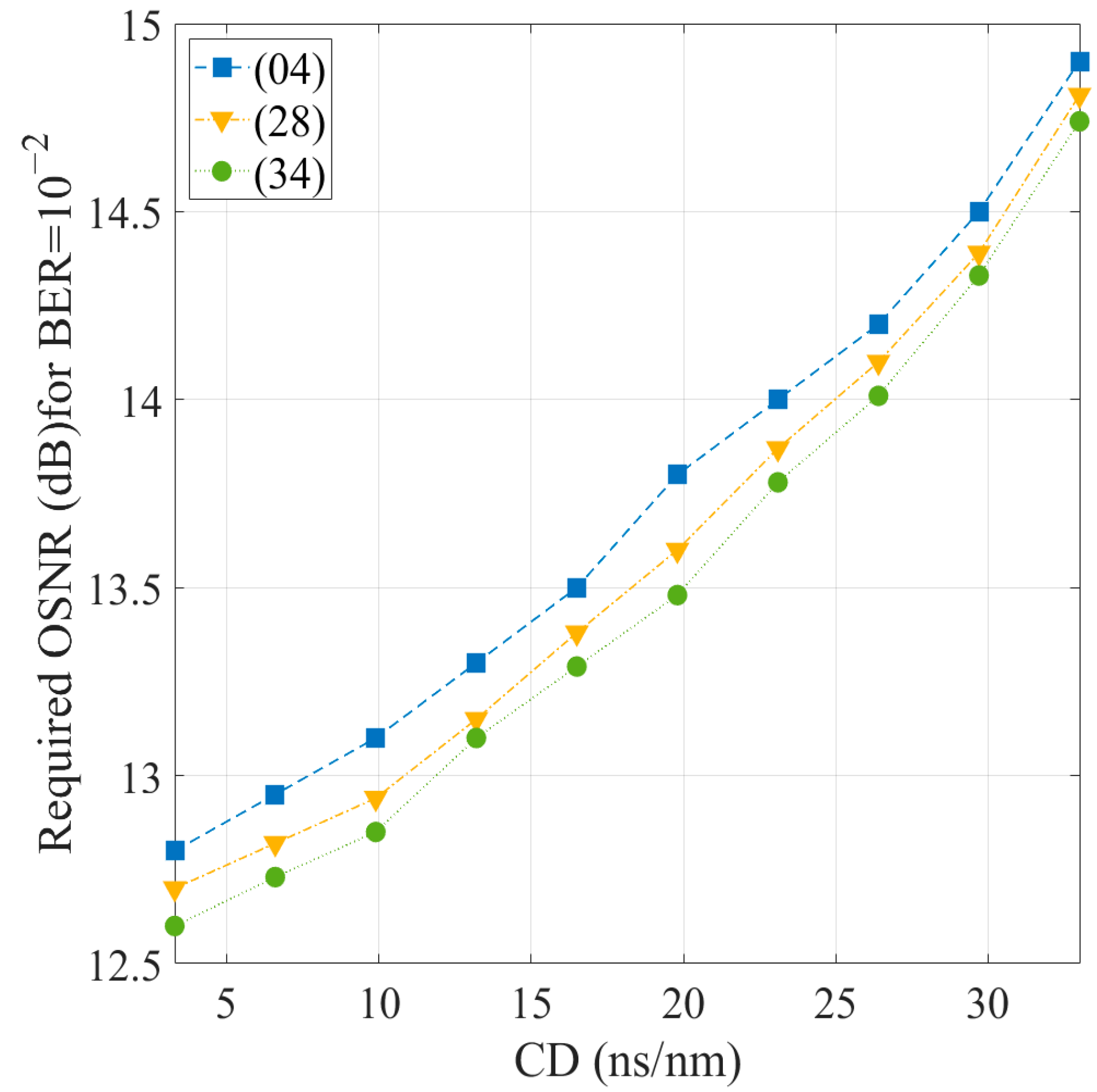
From the results of simulation and experiments, the filter in (28) and the filter in (34) can achieve better CDE, and under the same filter length, the latter’s performance will be better. Even though we mainly discuss the implementation complexity, compared between the two proposed schemes, because the particles need a certain amount of exploration time to find the optimal solution, the filter design complexity in (34) will be higher than (28). Moreover, when the length of the filter $N$ increases, it means that the dimensions of the particles, the number of populations, and the number of iterations are best also growing, which requires more search time to obtain the best solution. In summary, for short-distance communication conditions, we can use the CDE filter based on AMPSO. When the transmission distance increases, the CDE filter design based on SVDLS is more appropriate.

6. Conclusions

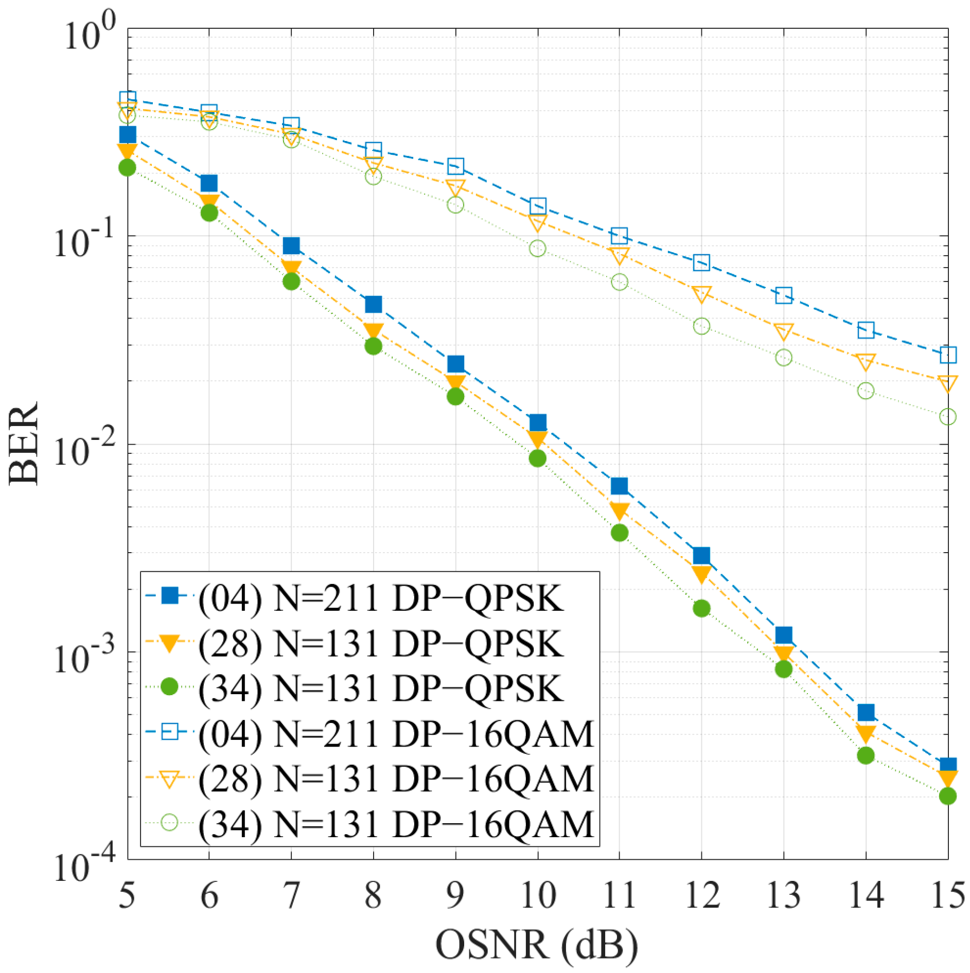
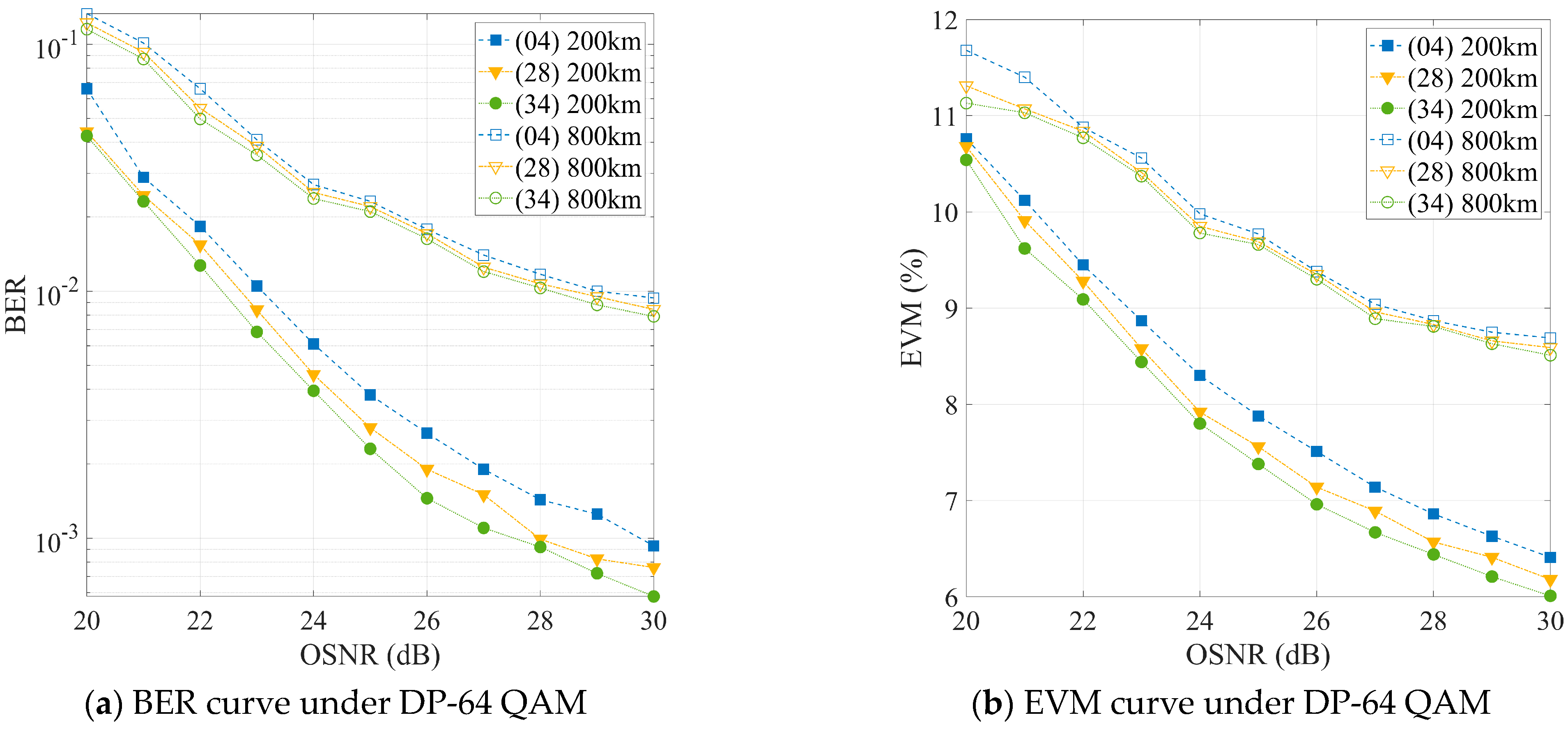
In this study, we proposed two schemes for linear damage equalization. The proposed method is suitable for linear modulation, including QPSK, 16 QAM, and 64 QAM, using AMSPO and SVDLS filter structures as DSP impairment equalization algorithms to deal with the CD in coherent optical communication systems. We provide simulation examples to compare with the widely used TD-CDE and FD-CDE filters. The results show that due to the influence of the pulse shaping filter, under the same accumulative CD, the two filter schemes we proposed require fewer taps than the existing filters, which reduces the complexity and cost of implementation. The two CDE schemes are evaluated on the 28 GBaud PDM-16 QAM experimental platform, and compared with the TD-CDE, the simulation results verify that the two proposed design schemes have lower SER.

We also compared the two proposed schemes. Considering factors such as equalization effect and design complexity, the application scenarios of two CDE schemes are given. In summary, the proposed methods are a promising solution for CDE.

References

1. Sun, X.; Zuo, Z.; Su, S.; Tan, X. Blind Chromatic Dispersion Estimation Using Fractional Fourier Transformation in Coherent Optical Communications. In Proceedings of the 2020 IEEE International Conference on Artificial Intelligence and Information Systems (ICAIIS), Dalian, China, 20–22 March 2020; Institute of Electrical and Electronics Engineers (IEEE): Piscataway, NJ, USA, 2020. [Google Scholar]
2. Dar, A.B.; Jha, R.K. Chromatic dispersion compensation techniques and characterization of fiber Bragg grating for dispersion compensation. Opt. Quantum Electron. 2017, 49, 1–35. [Google Scholar] [CrossRef]
3. Felipe, A.; de Souza, A.L.N. Chirp-Filtering for Low-Complexity Chromatic Dispersion Compensation. J. Lightwave Technol. 2020, 38, 2954–2960. [Google Scholar] [CrossRef]
4. Toms, S.; Andis, S.; Vjaceslavs, B.; Jurgis, P.; Sandis, S. Comparison of Dispersion Compensation Techniques for Real-Time up to 160 Gbit/s DWDM C-Band Transmission. Elektron. Elektrotech. 2020, 26, 85–93. [Google Scholar]
5. El-Nahal, F.I.; Abualoff, N.M. Coherent optical communication systems based on orthogonal frequency division multiplexing. Optoelectron. Lett. 2020, 16, 303–305. [Google Scholar] [CrossRef]
6. Yu, Y.; Yin, H.; Huang, Z. Simulation Study of DP-QPSK Coherent Detection Transmission System Based on Optisystem. Opt. Photon. J. 2020, 10, 134–140. [Google Scholar] [CrossRef]
7. Ba, J.; Huang, Z.; Shen, F.; Wei, J. Joint Estimation of Symbol Rate and Chromatic Dispersion Using Delayed Multiplier for Optical Performance Monitoring. Photonics 2021, 8, 58. [Google Scholar] [CrossRef]
8. Geyer, J.C.; Fludger, C.R.S.; Duthel, T.; Schulien, C.; Schmauss, B. Efficient frequency domain chromatic dispersion compensation in a coherent Polmux QPSK-receiver. In Proceedings of the 2010 Conference on Optical Fiber Communication (OFC/NFOEC), Collocated National Fiber Optic Engineers Conference, San Diego, CA, USA, 21–25 March 2010; pp. 1–3. [Google Scholar]
9. Xu, T.; Jacobsen, G.; Popov, S.; Li, J.; Wang, K.; Friberg, A.T. Normalized LMS digital filter for chromatic dispersion equalization in 112-Gbit/s PDM-QPSK coherent optical transmission system. Opt. Commun. 2010, 283, 963–967. [Google Scholar] [CrossRef]
10. Otuya, D.O.; Kasai, K.; Yoshida, M.; Hirooka, T.; Nakazawa, M. A single-channel 192 Tbit/s, 64 QAM coherent optical pulse transmission over 150 km using frequency-domain equalization. Opt. Express 2013, 21, 22808–22816. [Google Scholar] [CrossRef]
11. Pittalà, F.; Slim, I.; Mezghani, A.; Nossek, J.A. Training-Aided Frequency-Domain Channel Estimation and Equalization for Single-Carrier Coherent Optical Transmission Systems. J. Light. Technol. 2014, 32, 4849–4863. [Google Scholar] [CrossRef]
12. Yumin, L.; Yuhong, Z.; Yunfeng, P.; Zhizhong, Z. Equalization of Chromatic Dispersion Using Wiener Filter for Coherent Optical Receivers. IEEE Photonics Technol. Lett. 2015, 28, 1092–1095. [Google Scholar]
13. Zhang, N.; Yi, W.; Zheng, Z.; Cui, N.; Guo, R.; Qiu, L.; Zhang, X.; Xi, L.; Zhang, W.; Xu, H. Joint equalization of linear impairments using two-stage cascade Kalman filter structure in coherent optical communication systems. Opt. Commun. 2019, 453, 124398. [Google Scholar] [CrossRef]
14. Amiri, I.; Rashed, A.N.Z.; Kader, H.M.A.; Al-Awamry, A.; El-Aziz, I.A.A.; Yupapin, P.; Palai, G. Optical communication transmission systems improvement based on chromatic and polarization Mode dispersion compensation simulation management. Optik 2019, 207, 163853. [Google Scholar] [CrossRef]
15. Muhammad, F.; Ali, F.; Habib, U.; Usman, M.; Khan, I.; Kim, S. Time Domain Equalization and Digital Back-Propagation Method-Based Receiver for Fiber Optic Communication Systems. Int. J. Opt. 2020, 2020, 1–13. [Google Scholar] [CrossRef]
16. Spinnler, B. Equalizer Design and Complexity for Digital Coherent Receivers. IEEE J. Sel. Top. Quantum Electron. 2010, 16, 1180–1192. [Google Scholar] [CrossRef]
17. Poggiolini, P.; Carena, A.; Curri, V.; Forghieri, F. Evaluation of the computational effort for chromatic dispersion compensation in coherent optical PM-OFDM and PM-QAM systems. Opt. Express 2009, 17, 1385–1403. [Google Scholar] [CrossRef] [PubMed]
18. Martins, C.S.; Guiomar, F.P.; Amado, S.B.; Ferreira, R.M.; Ziaie, S.; Shahpari, A.; Teixeira, A.L.; Pinto, A.N. Distributive FIR-Based Chromatic Dispersion Equalization for Coherent Receivers. J. Light. Technol. 2016, 34, 5023–5032. [Google Scholar] [CrossRef]
19. Pillai, B.S.G.; Sedighi, B.; Guan, K.; Anthapadmanabhan, N.P.; Shieh, W.; Hinton, K.J.; Tucker, R.S. End-to-End Energy Modeling and Analysis of Long-Haul Coherent Transmission Systems. J. Light. Technol. 2014, 32, 3093–3111. [Google Scholar] [CrossRef]
20. Savory, S.J. Digital filters for coherent optical receivers. Opt. Express 2008, 16, 804–817. [Google Scholar] [CrossRef]
21. Taylor, M.G. Compact Digital Dispersion Compensation Algorithms. In Proceedings of the OFC/NFOEC 2008—2008 Conference on Optical Fiber Communication/National Fiber Optic Engineers Conference, Anaheim, CA, USA, 24–28 February 2008. [Google Scholar]
22. Qian, D.; Hu, J.; Wang, T.; Aono, Y.; Tajima, T. Chromatic Dispersion Compensation Using Sign Operations and Lookup Tables. US8718474B2, 29 November 2012. [Google Scholar]
23. Eghbali, A.; Johansson, H.; Gustafsson, O.; Savory, S. Optimal Least-Squares FIR Digital Filters for Compensation of Chromatic Dispersion in Digital Coherent Optical Receivers. J. Light. Technol. 2014, 32, 1449–1456. [Google Scholar] [CrossRef]
24. Agrawal, G.P. Fiber-Optic Communication Systems, 4th ed.; Wiley: Hoboken, NJ, USA, 2010. [Google Scholar]
25. Kidambi, S.S.; Ramachandran, R.P. Complex coefficient nonrecursive digital filter design using a least-squares method. IEEE Trans. Signal Process. 1996, 44, 710–713. [Google Scholar] [CrossRef]
26. Cui, L.; Tao, Y.; Deng, J.; Liu, X.; Xu, D.; Tang, G. BBO-BPNN and AMPSO-BPNN for multiple-criteria inventory classification. Expert Syst. Appl. 2021, 175, 114842. [Google Scholar] [CrossRef]
27. Mishra, B.; Kumar, A.; Zaburko, J.; Sadowska-Buraczewska, B.; Barnat-Hunek, D. Dynamic Response of Angle Ply Laminates with Uncertainties Using MARS, ANN-PSO, GPR and ANFIS. Materials 2021, 14, 395. [Google Scholar] [CrossRef]
28. Sun, D.; Wei, E.; Ma, Z.; Wu, C.; Xu, S. Optimized CNNs to Indoor Localization through BLE Sensors Using Improved PSO. Sensors 2021, 21, 1995. [Google Scholar] [CrossRef] [PubMed]
29. Xu, T.; Jacobsen, G.; Popov, S.; Forzati, M.; Martensson, J.; Mussolin, M.; Li, J.; Wang, K.; Zhang, Y.; Friberg, A.T. Frequency-Domain Chromatic Dispersion Equalization Using Overlap-Add Methods in Coherent Optical System. J. Opt. Commun. 2011, 32. [Google Scholar] [CrossRef]
Figure 1. Coherent optical communication system structure diagram.
Photonics 08 00478 g001
Figure 2. The OSNR penalty performance of the DP-QPSK and DP-16 QAM data. (a) The signal modulation format is DP-QPSK; (b) The signal modulation format is DP-16 QAM.
Photonics 08 00478 g002
Figure 3. The BER and the OSNR penalty performance of DP-QPSK data with different n values. (a) The BER vs. number of coefficients of the CDE filter; (b) The OSNR penalty performance vs. number of coefficients of the CDE filter.
Photonics 08 00478 g003
Figure 4. The BER performance of DP-QPSK and DP-16 QAM data with Ω [ 3 π / 8 , 3 π / 8 ] , the filter (4) has 211 taps, while filter (28) and (34) have 131 taps.
Photonics 08 00478 g004
Figure 5. The BER and EVM performance of the DP-64 QAM data. We compare the equalization performance of the filters of TD-CDE-FIR, SVDLS-FIR, and AMPSO-FIR under different OSNR when the same filter length n and the transmission distance are 200 km and 800 km. (a) Performance index of BER; (b) Performance index of EVM.
Photonics 08 00478 g005
Figure 6. The OSNR penalty performance of the 64 GBaud DP-QPSK data.
Photonics 08 00478 g006
Figure 7. The BER performance of the DP-QPSK and DP-64 QAM data. We compare the equalization performance of the filters of FD-CDE-FIR, SVDLS-FIR, and AMPSO-FIR under different OSNR. (a) The transmission distance of DP-QPSK modulation is 1000 km; (b) The transmission distance of DP-64 QAM modulation is 500 km.
Photonics 08 00478 g007
Figure 8. Experiment setup of 28-GBaud PDM-16 QAM transmission. ELC: external cavity laser; DP-MZM: dual-polarization Mach Zehnder modulator; AOS: acousto-optic switch; PS: polarization scrambler; OBPF: optical band-pass filter; VOA: carriable optical attenuator; SMF: standard single-mode fiber; TOF: tunable optical filter.
Photonics 08 00478 g008
Figure 9. SER vs. Transmitted Length for PDM-16 QAM signal (OSNR = 20.2 dB).
Photonics 08 00478 g009