Coherent Random-Modulated Continuous-Wave LiDAR Based on Phase-Coded Subcarrier Modulation

Abstract

A coherent random-modulated continuous-wave (RMCW) LiDAR transmits a lightwave modulated by a pseudo-random binary sequence (PRBS). The lightwave backscattered from targets is received and used to reconstruct the PRBS. Then, the time-of-flight is extracted by correlating the reconstructed PRBS and the original PRBS. We propose a coherent RMCW LiDAR based on phase-coded subcarrier modulation, in which the impacts of internal reflection and optical Doppler frequency shift (DFS) are mitigated. A continuous lightwave is amplitude-modulated by an RF signal which is phase-coded with a PRBS. Coherent detection is used in the receiver. A beat signal that consisted of a low-frequency signal and a high-frequency signal is obtained by a single balanced photodetector (BPD). The optical DFS can be directly extracted from the low-frequency signal. It is used to compensate for the frequency offset of PRBS, which is extracted from the high-frequency signal. In addition, the background noise caused by internal reflection is suppressed by averaging over successive measurement spots. In this paper, the performance of a coherent RMCW LiDAR is firstly analyzed by numeric simulations and demonstration experiments. Then, line-scanning measurements for moving targets are implemented to demonstrate the 3D imaging capability of the proposed coherent RMCW LiDAR.

1. Introduction

Light detection and ranging (LiDAR) is an active remote sensing technology that detects targets from backscattered light [1,2], In various applications, such as 3D imaging [3], automatic driving [4], and meteorology [5], LiDAR has been widely used, whereby the distance, velocity, and azimuth angle of targets can be simultaneously measured [6]. To measure the distance, the lightwave in a LiDAR is required to be time-varying modulated so that the time-of-flight (ToF) of the backscattered light can be extracted [1]. Typical LiDAR systems include pulsed [7], phase-modulated [8], frequency-modulated continuous-wave (FMCW) [9,10], and random-modulation continuous-wave (RMCW) LiDAR [11,12]. The RMCW LiDAR was firstly proposed by Takeachi in 1983, in which amplitude-modulation and incoherent detection are used [12]. The RMCW LiDAR uses a pseudo-random binary sequence (PRBS) to modulate the lightwave [13,14]. In the receiver, the PRBS is reconstructed from the intensity of the backscattered light. The time-of-flight is obtained from the correlation between the original PRBS and the reconstructed PRBS [15]. Since the PRBS only correlates with itself, the RMCW lidar is insensitive to spurious light, which includes sunlight, lamplight, and the light of other lidars. As a result, the RMCW LiDAR is immune to interference with other lidars. However, in an incoherent RMCW LiDAR, the optical phase of backscattered light cannot be obtained so that laser Doppler velocimetry is unable to be achieved.

Coherent RMCW LiDAR is an approach to simultaneously implement ranging and velocimetry [16,17,18]. In a coherent RMCW LiDAR, the transmitted light is coded by a PRBS. The backscattered light beats with a local oscillator (LO) to obtain the reconstructed PRBS. Since coherent detection is used, a coherent LiDAR has high sensitivity [19] and is sensitive to the phase variation of backscattered light [17]. Therefore, optical Doppler frequency shift (DFS) can be extracted from the beating signals to estimate the relative radial velocity of targets [20]. However, in a coherent RMCW LiDAR, the optical DFS results in a frequency offset between the original PRBS and the reconstructed PRBS [16,17]. The frequency offset may degrade the correlation of PRBS so that the distance cannot be extracted.

To mitigate the impacts of the optical DFS, time-multiplexing is used, by which a continuous-wave signal is inserted into two adjacent PRBSs [16]. The approach requires only one phase modulator and one non-quadrature demodulator, so the hardware is simple. However, the measurement time per pixel is long since the periods of the signal are increased. The computational complexity of the approach is also relatively high. Another approach is using a quadrature demodulator and amplitude modulation, in which the amplitude of the lightwave is coded by a PRBS [17]. The delayed PRBS and optical DFS can be separately reconstructed from the amplitude and phase of the backscattered light via the quadrature demodulator [21,22]. However, the quadrature demodulator consists of a 90-degree optical hybrid and two balanced photodetectors (BPDs), which is complex and entails a high cost.

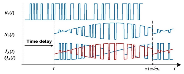
In this paper, we propose a coherent RMCW LiDAR based on phase-coded subcarrier modulation. An RF signal is firstly phase-coded by a PRBS and then used to modulate a continuous lightwave in an intensity modulator. Since subcarrier modulation is used, the beat signal between the backscattered light and the LO consists of a low-frequency signal and a high-frequency signal. The optical DFS can be extracted from the low-frequency signal, while the delayed PRBS with a frequency offset is reconstructed from the high-frequency signal. The performance of coherent RMCW LiDARs is firstly analyzed by numeric simulations. Then, a 1550-nm coherent RMCW LiDAR is built, in which a 1.25-GHz RF signal phase-coded with a 12-bit M-sequence is used as the subcarrier. The optical DFS is measured and then used to compensate for the frequency offset in the reconstructed PRBS. Meanwhile, the background noise caused by internal reflection is suppressed by averaging over successive measurement spots. Moreover, line-scanning measurements are implemented to demonstrate the 3D imaging capability of the coherent RMCW LiDAR for moving targets. The proposed coherent RMCW LiDAR can be used for automatic driving.

2. Principle of Coherent RMCW LiDARs

2.1. Basic Concepts of RMCW LiDARs

An RMCW LiDAR estimates the time delay of backscattered light by calculating the correlation between the reconstructed PRBS and the original PRBS. Typically, the PRBS is used to phase-code the lightwave in a coherent RMCW LiDAR [23]. The light backscattered from the target is given as

E_p(t) = E₀ exp{i (ω_c + ω_d) (t − τ) + β cos[θ_n(t − τ)]}

(1)

in which β is the modulation factor, τ is the time delay of backscattered light, ω_c and ω_d are the angular frequency of the optical carrier and the optical DFS. θ_n(t) is the PRBS which is shown in the top of Figure 1. To achieve maximum modulation depth, the value of θ_n(t) is set to 0 or π. Using coherent detection, the backscattered light beats with an LO in a BPD. From the beat signal, the PRBS can be reconstructed as

S_p(t) = sin{β cos[θ_n(t − τ)] + ω_d (t − τ) + φ]}

(2)

The correlation C(kT_s) of the reconstructed PRBS and θ_n(t) can be calculated as

$$C\left(k{T}_s\right)={{\displaystyle \sum }}_{n=0}^R{S}_p\left(n{T}_s\right)\cos \left\{{\theta }_n\left[\left(n-k\right) T_s\right]\right\}$$

(3)

where k∈Z represents relative delay, T_s is the sampling period, R is the sequence length. It should be noted that the optical DFS and θ_n(t) are coupled with each other in S_P(t), which is shown in the middle of Figure 1. The optical DFS causes a frequency offset in the reconstructed PRBS, which impairs the peak-sideband-ration (PSR) of the normalized correlation. If the frequency offset is large enough, laser ranging may be disabled [16,17].

To decouple the PBRS and optical DFS, amplitude modulation and an optical coherent receiver can be used. The backscattered light is given by

E_A(t) = E₀ sin{β cos[θ_n(t − τ)]} exp[i (ω_c + ω_d) (t − τ) + φ]

(4)

The two outputs of the optical coherent receiver can be obtained as

I_A(t) = sin{β cos[θ_n(t − τ)]} sin[ω_d (t − τ) + φ]

(5)

Q_A(t) = sin{β cos[θ_n(t − τ)]} cos[ω_d (t − τ) + φ]

(6)

which are shown in the bottom of Figure 1. Based on the two outputs, a complex signal is reconstructed as

S_A(t)= sin{β cos[θ_n(t − τ)]} exp [i ω_d (t − τ) + φ]

(7)

Therefore, the PRBS and optical DFS can be respectively reconstructed via the I/Q demodulation. The correlation is calculated as

$$C\left(k{T}_{s}T\mathrm{s}\right)={{\displaystyle \sum }}_{n=0}^R|S_{\mathrm{A}}\left(n{T}_s\right)|\cos \left\{{\theta }_n\left[\left(n-k\right)T_s\right]\right\}$$

(8)

Since the optical DFS only impacts the phase of S_A(t), the correlation C(kT_s) can be used for laser ranging even though the target is moving [17]. However, the optical coherent receiver enhances the cost and complexity of coherent RMCW LiDARs.

2.2. Coherent RMCW LiDARs Based on Phase-Coded Subcarrier Modulation

Since it significantly degrades the performance of RMCW LiDARs, the optical DFS must be real-time compensated to remove the frequency offset. For simultaneously ranging and velocimetry, an RMCW LiDAR based on phase-coded subcarrier modulation is proposed. An RF signal is used as the subcarrier which is phase-coded by a PRBS [24]. The phase-coded subcarrier V_n(t) = cos[${\omega }_{\mathrm{RF}}$t + θ_n(t)] is shown in the top of Figure 2, which is used to modulate the lightwave in an intensity modulator. The backscattered light in the coherent RMCW LiDAR can be written as

$$E_{\mathrm{sub}}=E_0\cos \left\{\beta \cos \right[{\omega }_{\mathrm{RF}}(t-\tau )+{\theta }_n(t-\tau )+\phi ]\left\}\exp \right[i({\omega }_{\mathrm{c}}+{\omega }_{\mathrm{d}}{)}_{}(t-\tau \left)\right]$$

(9)

where ${\omega }_{\mathrm{RF}}$ is the angular frequency of the subcarrier and φ is the phase bias of the intensity modulator. The beat signal between the backscattered light and the LO can be expressed as:

$$i_{\mathrm{sub}}\left(t\right)\propto \cos \left[{\omega }_{\mathrm{d}}\right(t-\tau \left)\right]\cos \left\{\beta \cos \right[{\omega }_{\mathrm{RF}}(t-\tau )+{\theta }_n(t-\tau )\left]\right\}$$

(10)

Since subcarrier modulation is used, the backscattered light consists of an optical carrier and optical sidebands. The phase-coded subcarrier is conveyed by the optical sidebands. A beat signal that consisted of a low-frequency signal and a high-frequency signal is generated, which can be respectively written as

i_low(t)∝J₀(β) cos[ω_d (t − τ)] cos(φ)

(11)

$$i_{\mathrm{high}}\left(t\right)\propto J_1\left(\beta \right)\cos \left[{\omega }_{\mathrm{RF}}\right(t-\tau )+{\theta }_n(t-\tau \left)\right]\cos \left[{\omega }_{\mathrm{d}}\right(t-\tau \left)\right]\sin \left(\phi \right)$$

(12)

which are shown in the middle and bottom of Figure 2. The low-frequency signal is the beat signal between the backscattered optical carrier and the LO. On the other hand, the high-frequency signal is a delayed PRBS with a frequency offset, which is the beat signal of the backscattered optical sideband and the LO. The optical DFS is measured from the low-frequency signal and used to compensate for the frequency offset in the high-frequency signal. Finally, the phase-coded subcarrier is reconstructed as

$$S_{\mathrm{sub}}\left(t\right)=\cos \left[{\omega }_{\mathrm{RF}}\right(t-\tau )+{\theta }_n(t-\tau \left)\right]\sin \left(\phi \right)$$

(13)

which is used to calculate the correlation with v(t) to extract the distance of targets. Therefore, ranging and velocimetry are simultaneously achieved by a coherent RMCW LiDAR using the phase-coded subcarrier modulation. Moreover, since the power of the low-frequency signal can be reduced by adjusting the phase bias of the intensity modulator, most of the optical power can be used for phase-coded optical sidebands so that the detection range can be enhanced. The proposed method provides a simple coherent RMCW LiDAR using a single BPD.

3. Numeric Simulations of Coherent RMCW LiDARs

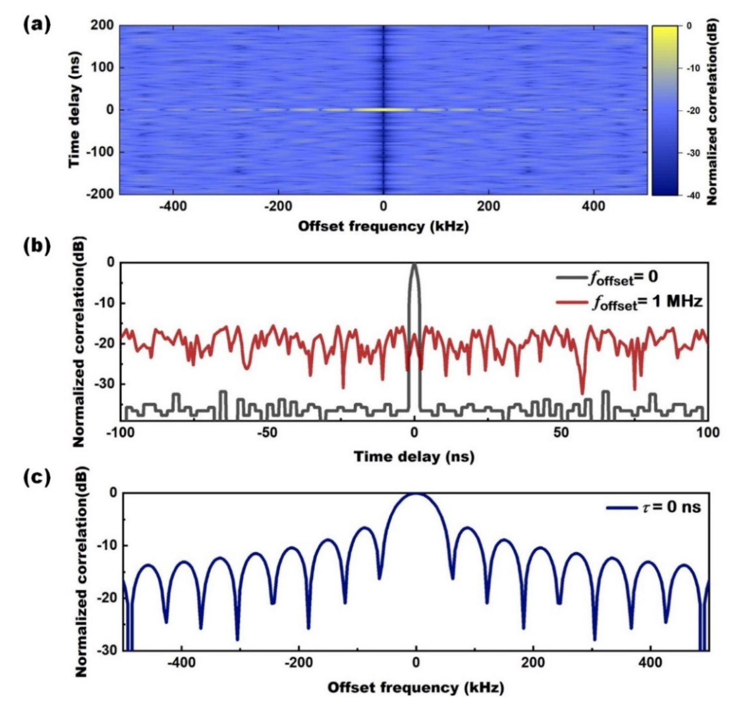
To evaluate the performance of RMCW LiDARs, the normalized ambiguity function (NAF) [25] for the PRBS is firstly calculated. A 500-M/bit/s 12-bit M-sequence is used as the PRBS [12] and the NAF is shown in Figure 3a. At zero offset frequency, the NAF illustrates the auto-correlation of the M-sequence (Figure 3b), which shows a peak at zero time delay. The peak width is equal to code-width (T₀) so that the range resolution of the RMCW LiDAR is equal to cT₀/2. However, as shown in Figure 3c, the NAF at zero time delay is a function of offset frequency. At 100 kHz offset frequency, the correlation decrease to −8 dB. At 1-MHz offset frequency, the correlation (red line in Figure 3b) shows no peaks at zero time delay, which indicates that ranging is no longer feasible. In a coherent RMCW LiDAR, the offset frequency is equal to the optical DFS. For a 1550 nm RMCW LiDAR, the optical DFS for a 1.5-m/s target is around 1 MHz, which is large enough to disable laser ranging.

Then, the performance of the proposed coherent RMCW LiDAR is analyzed by numeric simulations. The schematic diagram of the coherent RMCW LiDAR is shown in Figure 4. A 1550-nm continuous lightwave is split into two parts. One part of the light is used as the LO and the other part is modulated by a phase-coded subcarrier in a Mach-Zehnder modulator. In the receiver, a BPD is used to detect the beat signal between the backscattered light and the LO. The power of the transmitted lightwave and the LO is 100 mW and 2 mW. The modulation signal is a 1.25-GHz RF signal phase-coded with a 500-Mbits/s 12-bit M-sequence. The bandwidth, responsivity, transimpedance gain, and minimum noise equivalent power of the BPD are 1.6 GHz, 0.85 A/W, 16×10³ V/A, and 9.3 pW/Hz^1/2, respectively. The sampling rate of the analog-to-digital converter (ADC) is 5 GSa/s. Although the simulation is not as comprehensive as that given in Ref. [23], it clearly estimates the impacts of internal reflection and optical DFS.

Figure 5 shows the simulations with internal reflection. In a practical system, the intensity of the internal reflection is fixed, while the intensities of the backscattered light from targets are different. Therefore, the power of the internal reflection is set to 1.5 nW, while the power of the backscattered light is set respectively to 1.5 nW, 0.15 nW, and 0.015 nW. Shown as the black line in Figure 3b, the theoretical SNR of the correlation at 0-Hz offset frequency is 30 dB. However, in practical RMCW lidars, the SNR is only less than 15 dB, which is caused by the noise of the photodetector and the relative intensity noise of the laser source. As a result, if the intensity of the internal reflection is high, the noise floor of the correlation is determined by the internal reflection. Thus, the signal of weak backscattered light may be submerged by the background noise [14,26]. As shown in Figure 5, the internal reflection is at 2 m, while the target is at 10 m. The length of uncompensated fiber is included in the distance. It can be observed that the lower is the power of the backscattered light, the smaller SNR is obtained for the signals of targets. In Figure 5c, if the power of internal reflection is 20 dB higher than the backscattered light, the correlation signal is fully submerged by the noise caused by the internal reflection. Therefore, the internal reflection has impacts on the sensitivity of RMCW LiDARs, which impairs the long-range detection capability.

The impacts of optical DFS on the coherent RMCW LiDAR are illustrated in Figure 6. In the simulations, the power of the backscattered light is set to 1.5 nW and no internal reflection exists. The velocities of the target are set to 0 m/s, 0.2 m/s, and 0.5 m/s in Figure 6a–c, respectively. With increasing velocity, the optical DFS significantly reduces the SNR of the correlation results. As shown in Figure 6c, for the 1550-nm RMCW LiDAR, there is no obvious peak in the correlation results so that the distance cannot be extracted if the velocity is larger than 0.5 m/s. It should be noted that the velocity capacity of the coherent RMCW LiDAR is much smaller than the incoherent RMCW LiDAR since the optical DFS causes a larger frequency offset than the microwave Doppler shift. In practical applications, the velocity of the target is always larger than 0.5 m/s which makes the coherent RMCW LiDAR inapplicable in the automatic drive. Therefore, the impacts of internal reflection and optical DFS must be mitigated to make the coherent RMCW lidar applicable for the automatic drive. The comprehensive simulations on the detection statistics of coherent RMCW lidars can be simulated following Ref. [23].

4. Experiments and Results

A coherent RMCW LiDAR is built. To demonstrate the 3D imaging capability, a galvanometer scanning system is added behind the telescope to steer the laser beam. The other parts of the LiDAR are the same as Figure 4. The phase-coded subcarrier is generated by an arbitrary waveform generator (AWG, Tektronix AWG70001A). A 1550-nm lightwave from a narrow line-width laser ((TeraXion PS-NLL)) is modulated by the phase-coded subcarrier in an MZM (Fujitsu FTM7938EZ). The modulated lightwave is amplified to 100 mW and transmitted by a telescope with a 10-mm spot diameter. The backscattered light beats with a 2-mW local oscillator in a BPD (Thorlabs PDB480C-AC). The outputs of the BPD are recorded by an oscilloscope (Agilent, DSO9404) with a sampling rate of 5 GSa/s. The recorded signals are processed offline to extract the distance of targets. In addition, an optical spectrum analyzer (OSA, Yokogawa AQ6370D) is used to monitor the optical spectrum.

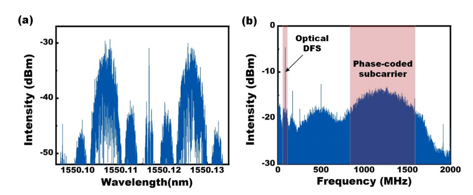
Figure 7a shows the optical spectrum of the transmitted lightwave, in which the subcarrier is a 1.25-GHz RF signal phase-coded by a 500-Mbit/s M-sequence. Since the optical carrier is suppressed in the MZM, most of the optical power is used for the optical sidebands which convey the phase-coded subcarrier. It is helpful to enhance the detection range. Figure 7b shows the beat signal between the backscattered light and the LO. An 85-MHz optical DFS is simulated by an acoustic-optic modulator (AOM), which is shown in the low-frequency region. The frequency of the subcarrier is much higher than the optical DFS so that the subcarrier can be readily separated by a filter. Finally, the optical DFS is individually measured from the low-frequency signal, which can be used to compensate for the phase-coded subcarrier in the high-frequency signal.

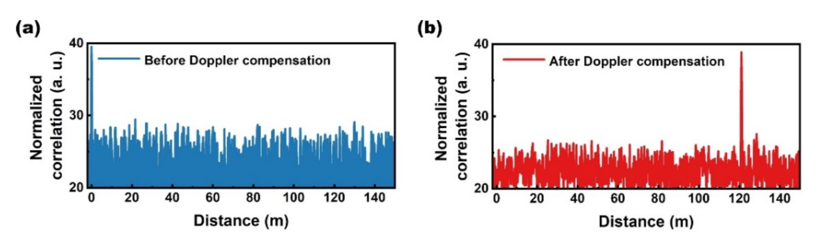
An experiment is implemented to demonstrate the DFS mitigation in RMCW lidar, in which a 77-MHz optical DFS is simulated by the AOM and the length of a fiber spool is measured. Figure 8 shows the measurement results. The normalized correlation before Doppler compensation (blue line) only shows a peak at 0 m, which is caused by the internal reflection. It is impossible to extract the distance information due to the optical DFS. However, after Doppler compensation, the normalized correlation (red line) shows a peak at around 120 m. Meanwhile, the signal caused by internal reflection disappears. Therefore, the feasibility of the DFS mitigation is demonstrated.

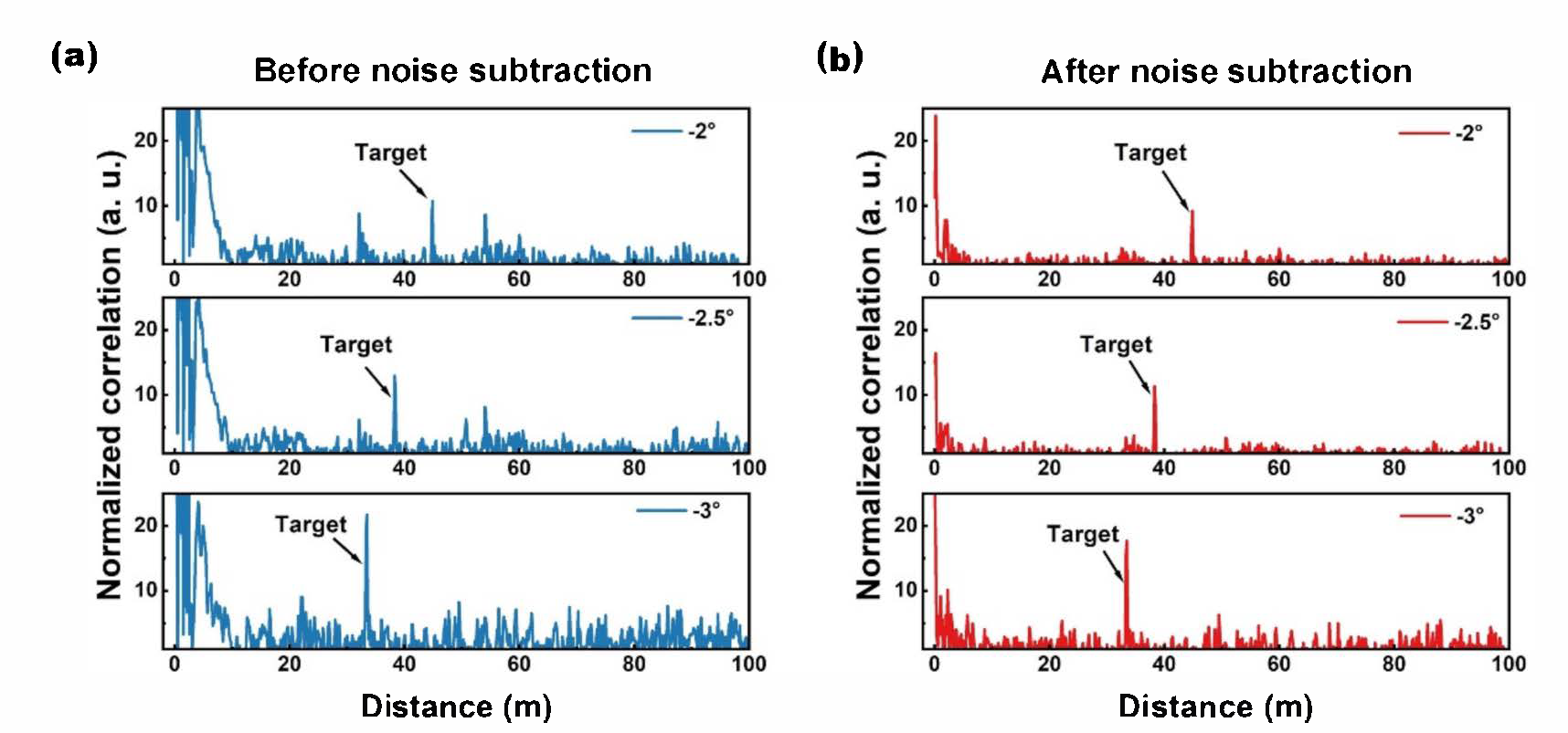
Since the internal reflection signal experiences no optical DFS, the impacts of internal reflection can be mitigated by Doppler compensation for the moving targets. However, for static targets, no Doppler compensation is implemented, so the internal reflection still needs to be suppressed. Figure 9a shows the normalized correlation for backscattered light in different directions. Although the normalized correlations show different signals of targets, similar background noise is observed in all of the normalized correlations, which is caused by the same internal reflection. The signals caused by internal reflection can be extracted by averaging the recovered signals at different directions, which is then used as a noise template. Figure 9b shows the normalized correlations after noise subtraction, in which the noise template is subtracted from the recovered signal at every measurement spot. The intense signals around 0 m are largely reduced in the normalized correlations. Meanwhile, the background noise is suppressed so that the signals of targets are obviously shown.

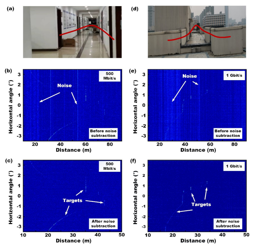
To demonstrate the capability of 3D imaging, the laser beam is line-scanned by the galvanometer scanning system. The field-of-view (FOV) angle is directly derived from the beam steering angle. Since the memory depth of the oscilloscope is limited, the FOV of the recoded data is less than ±5. Figure 10 shows the results for the line-scanning measurements, in which the field-of-view (FOV) angle and scanning rate are ±3.5 and 25 Hz, respectively. Figure 10a,d are the photographs of the surroundings for the 3D imaging, in which the red lines are the scanning lines. Figure 10b,c are the measurement results in the corridor shown as Figure 10a, in which a 500-Mbits/s M-sequence is used. Figure 10d,f are the measurement results for outdoor buildings, shown as Figure 10d, in which a 1-Gbits/s M-sequence is used. The distance resolution for the 1-Gbits/s signal is around 15 cm, while it is 30 cm for the 500-Mbits/s signal.

Due to the internal reflection, background noise is shown in Figure 10b,e, which significantly impairs the SNR of the correlation. For example, in Figure 10e, the signal of targets at around 20 m is almost submerged by the background noise. It should be noted that the noise caused by internal reflection shows the same pattern in the correlation results in different directions. Therefore, vertical lines are shown in Figure 10b,e, which are higher than the signal of targets. To mitigate the impacts of internal reflection, an averaged signal of 20 successive measurement spots is used as a noise template, which is then subtracted from the measured signal in every spot. Figure 10c,f show the correlation results after noise subtraction, in which some signals of targets are indicated by the arrows. The noise signals are significantly reduced so the signals at around 20 m are clearly shown in Figure 10e. Since the noise is reduced, the sensitivity of the coherent RMCW LiDAR is largely enhanced so that the detection range is lengthened.

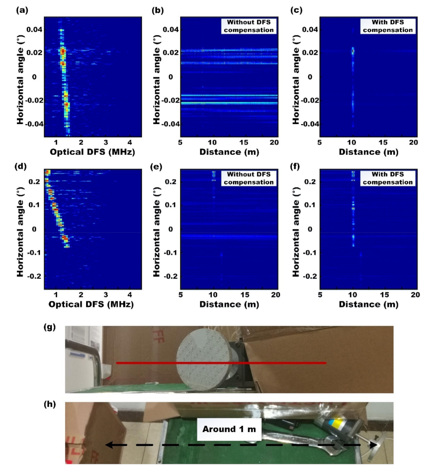
Moreover, a spinning disk is line-scanning measured to demonstrate the 3D imaging capability of the LiDAR for moving targets. To enhance the reflectivity, the spinning disk is covered by a reflective tape, which is shown in Figure 11g. In Figure 11a–c, the FOV angle and scanning rate are ±0.05 and 10 Hz, respectively. The optical DFS of the backscattered light is real-time measured from the low-frequency signal, which is shown in Figure 11a. Without DFS compensation, the correlation results of the high-frequency signal show no obvious peaks in Figure 11b due to the frequency offset caused by the optical DFS. To measure the distance of the spinning disk, the optical DFS measured in Figure 11a is used to compensate for the frequency offset in the high-frequency signal. After DFS compensation [17], peaks at around 10 m are shown in Figure 11c, which demonstrates that 3D imaging of the moving targets is achieved by the proposed LiDAR.

In Figure 11d–f, a target that consisted of a spinning disk and a static box is measured, in which the FOV angle and scanning rate are ±0.25 and 50 Hz, respectively. The targets are shown in Figure 11g,h. The center of the spinning disk is at 0.2 and the distance between the disk and the box is around 1 m. Since the laser beam scans from the center to the edge of the disk, the measured optical DFS increases to 1.5 MHz from 0.2 to −0.1. Meanwhile, peaks in the correlation results gradually fade from 0.2 to −0.1 in Figure 11e due to the increasing frequency offset. In contrast, the correlation results always show peaks at around 11 m from −0.1 to −0.25 since the box is static. To recover the signals for the moving targets, DFS compensation is used based on the real-time measured optical DFS. The correlation results after DFS compensation is shown in Figure 11f, where the signals for the spinning disk and static box can be simultaneously obtained, at around 10 m and 11 m, respectively. Meanwhile, the signal at 10 m is much intense than that at 11 m, which indicates that the reflectivity of the spinning disk is higher than the box. Moreover, the impacts of optical DFS are well mitigated by the real-time DFS compensation so that the proposed RMCW LiDAR can be used for the 3D imaging of moving targets. Compared with ToF LiDARs, the proposed coherent RMCW lidar can simultaneously measure the velocity and distance of the target. On the other hand, compared with FMCW LiDARs, the coherent RMCW lidar requires no frequency-swept laser source, in which the linear frequency sweeping is difficult to achieve. Therefore, RMCW LiDARs have potential applications in automatic driving.

5. Conclusions

In conclusion, the principle of coherent RMCW LiDARs is theoretically analyzed, which indicates that the internal reflection and optical DFS impair the performance of the LiDARs. To mitigate the impacts of optical DFS, a coherent RMCW LiDAR based on phase-coded subcarrier modulation is proposed. The frequency offset subcarrier and the optical DFS can be separately obtained from the high-frequency signal and the low-frequency signal, respectively. Then, the measured optical DFS is used to compensate for the frequency offset in the high-frequency signal. Finally, the phase-coded subcarrier is reconstructed and used to measure the distance of targets. On the other hand, the impact of internal reflection is mitigated by subtracting the averaged signal of 20 successive measurement spots from every measurement spot. A demonstration system for the proposed coherent RMCW LiDAR is built. Line-scanning measurements are implemented to demonstrate the 3D imaging capability. The noise signals are well suppressed so that the weak backscattered signal can be extracted. Using DFS compensation, the proposed coherent RMCW LiDAR is applicable for the 3D imaging of moving and static targets, by which the 3D coordinate and radial velocity can be simultaneously measured.

References

1. Amann, M.-C.; Bosch, T.; Lescure, M.; Myllylae, R.; Rioux, M. Laser ranging: A critical review of unusual techniques for distance measurement. Opt. Eng. 2001, 40, 10–19. [Google Scholar]
2. McManamon, P. Review of ladar: A historic, yet emerging, sensor technology with rich phenomenology. Opt. Eng. 2012, 51, 060901. [Google Scholar] [CrossRef] [Green Version]
3. Schwarz, B. Mapping the world in 3D. Nat. Photonics 2010, 4, 429–430. [Google Scholar] [CrossRef]
4. Rasshofer, R.H.; Gresser, K. Automotive radar and lidar systems for next generation driver assistance functions. Adv. Radio Sci. 2005, 3, 205–209. [Google Scholar] [CrossRef] [Green Version]
5. Käsler, Y.; Rahm, S.; Simmet, R.; Kühn, M. Wake measurements of a multi-mw wind turbine with coherent long-range pulsed Doppler wind lidar. J. Atmos. Ocean. Technol. 2010, 27, 1529–1532. [Google Scholar] [CrossRef] [Green Version]
6. Behroozpour, B.; Sandborn, P.A.M.; Wu, M.C.; Boser, B.E. Lidar system architectures and circuits. IEEE Commun. Mag. 2017, 55, 135–142. [Google Scholar] [CrossRef]
7. Liu, J.; Sun, Q.; Fan, Z.; Jia, Y. TOF Lidar development in autonomous vehicle. In Proceedings of the 2018 IEEE 3rd Optoelectronics Global Conference (OGC), Shenzhen, China, 4–7 September 2018; pp. 185–190. [Google Scholar]
8. He, H.; Sun, J.; Lu, Z.; Xu, M.; Lao, C.; Han, R.; Cai, X.; Li, Y. Phase-shift laser range finder technique based on optical carrier phase modulation. Appl. Opt. 2020, 59, 5079–5085. [Google Scholar] [CrossRef] [PubMed]
9. Anderson, J.; Massaro, R.; Curry, J.; Reibel, R.; Nelson, J.; Edwards, J. LADAR: Frequency-modulated, continuous wave laser detection and ranging. Photogram. Eng. Remote Sens. 2017, 83, 721–727. [Google Scholar] [CrossRef]
10. Martin, A.; Dodane, D.; Leviandier, L.; Dolfi, D.; Naughton, A.; O’Brien, P.; Spuessens, T.; Baets, R.; Lepage, G.; Verheyen, P.; et al. Photonic integrated circuit-based FMCW coherent lidar. J. Lightw. Technol. 2018, 36, 4640–4645. [Google Scholar] [CrossRef]
11. Nagasawa, C.; Abo, M.; Yamamoto, H.; Uchino, O. Random modulation cw lidar using new random sequence. Appl. Opt. 1990, 29, 1466–1470. [Google Scholar] [CrossRef] [PubMed]
12. Takeuchi, N.; Sugimoto, N.; Baba, H.; Sakurai, K. Random modulation cw lidar. Appl. Opt. 1983, 22, 1382–1386. [Google Scholar] [CrossRef] [PubMed]
13. Li, F.; Li, T.; Fang, X.; Tian, B.; Dou, X. Pseudo-random modulation continuous-wave lidar for the measurements of mesopause region sodium density. Opt. Express 2021, 29, 1932–1944. [Google Scholar] [CrossRef] [PubMed]
14. Rybaltowski, A.; Taflove, A. Superior signal-to-noise ratio of a new AA1 sequence for random-modulation continuous-wave lidar. Opt. Lett. 2004, 29, 1709–1711. [Google Scholar] [CrossRef] [PubMed]
15. Ai, X.; Nock, R.; Rarity, J.G.; Dahnoun, N. High-resolution random-modulation cw lidar. Appl. Opt. 2011, 50, 4478–4488. [Google Scholar] [CrossRef]
16. Banzhaf, S.; Waldschmidt, C. Phase-code-based modulation for coherent lidar. IEEE Trans. Veh. Technol. 2021, 70, 9886–9897. [Google Scholar] [CrossRef]
17. Spollard, J.T.; Roberts, L.E.; Sambridge, C.S.; McKenzie, K.; Shaddock, D.A. Mitigation of phase noise and Doppler-induced frequency offsets in coherent random amplitude modulated continuous-wave LiDAR. Opt. Express 2021, 29, 9060–9083. [Google Scholar] [CrossRef]
18. Xu, Z.; Tang, L.; Zhang, H.; Pan, S. Simultaneous real-time ranging and velocimetry via a dual-sideband chirped lidar. IEEE Photonics Technol. Lett. 2017, 29, 2254–2257. [Google Scholar] [CrossRef]
19. Shemer, K.; Bashan, G.; Diamandi, H.H.; London, Y.; Raanan, T.; Israelashvili, Y.; Charny, A.; Cohen, I.; Bergman, A.; Levanon, N.; et al. Sequence-coded coherent laser ranging with high detection sensitivity. OSA Contin. 2020, 3, 1274–1282. [Google Scholar] [CrossRef]
20. Karlsson, C.J.; Olsson, F.Å.A.; Letalick, D.; Harris, M. All-fiber multifunction continuous-wave coherent laser radar at 1.55 µm for range, speed, vibration, and wind measurements. Appl. Opt. 2000, 39, 3716–3726. [Google Scholar]
21. Gao, S.; O’Sullivan, M.; Hui, R. Complex-optical-field lidar system for range and vector velocity measurement. Opt. Express 2012, 20, 25867–25875. [Google Scholar] [CrossRef]
22. Xu, Z.; Zhang, H.; Chen, K.; Zhu, D.; Pan, S. FMCW Lidar Using Phase-Diversity Coherent Detection to Avoid Signal Aliasing. IEEE Photonics Technol. Lett. 2019, 31, 1822–1825. [Google Scholar] [CrossRef]
23. Sambridge, C.S.; Spollard, J.T.; Sutton, A.J.; McKenzie, K.; Roberts, L.E. Detection statistics for coherent RMCW LiDAR. Opt. Express 2021, 29, 25945–25959. [Google Scholar] [CrossRef] [PubMed]
24. Bashkansky, M.; Burris, H.R.; Funk, E.E.; Mahon, R.; Moore, C.I. RF phase-coded random-modulation LIDAR. Opt. Commun. 2004, 231, 93–98. [Google Scholar] [CrossRef]
25. Farnane, K.; Minaoui, K.; Rouijel, A.; Aboutajdine, D. Analysis of the ambiguity function for phase-coded waveforms. In Proceedings of the 2015 IEEE/ACS 12th International Conference of Computer Systems and Applications (AICCSA), Marrakech, Morocco, 17–20 November 2015; pp. 1–4. [Google Scholar]
26. Rybaltowski, A.; Taflove, A. Signal-to-noise ratio in direct-detection mid-infrared Random-Modulation Continuous-Wave lidar in the presence of colored additive noise. Opt. Express 2001, 9, 386–399. [Google Scholar] [CrossRef]
Figure 1. Schematic illustration of waveforms for θn(t), SP(t), IA(t) (red line), and QA(t) (blue line).
Photonics 08 00475 g001
Figure 2. Schematic illustration of waveforms for Vn(t), ilow(t), and ihigh(t).
Photonics 08 00475 g002
Figure 3. (a) Normalized ambiguity function (NAF) of a 12-bit M-sequence as a function of time delay and offset frequency. (b) Normalized correlation with 0-Hz and 1-MHz offset frequency. (c) Normalized correlation at 0-ns time delay as a function of offset frequency.
Photonics 08 00475 g003
Figure 4. Schematic configuration of the proposed coherent RAMCW LiDAR. LD: laser diode, OC: optical coupler, MZM: Mach-Zehnder modulator, BPD: balanced photodetector, ADC: analog-to-digital converter, DSP: digital signal processor.
Photonics 08 00475 g004
Figure 5. Numeric simulations for the coherent RMCW LiDAR in presence of internal reflection. The internal reflection is at 2 m, while the target is at 10 m. The power of the internal reflection is 1.5 nW. The power of the backscattered signal is (a) 1.5 nW, (b) 0.15 nW and (c) 0.015 nW.
Photonics 08 00475 g005
Figure 6. Numeric simulations for the coherent RMCW LiDAR to detect moving targets with different velocities. The velocity of the target is (a) 0 m/s, (b) 0.2 m/s and (c) 0.5 m/s.
Photonics 08 00475 g006
Figure 7. (a) Optical spectrum of the transmitted lightwave. (b) Spectrum of the beat signal, in which an 85-MHz optical DFS is simulated by an acoustic-optic modulator.
Photonics 08 00475 g007
Figure 8. Normalized correlation (a) before Doppler compensation and (b) after Doppler compensation. A 77-MHz optical DFS is simulated by an AOM and the length of a fiber spool is measured.
Photonics 08 00475 g008
Figure 9. Normalized correlation (a) before noise subtraction and (b) after noise subtraction The normalized correlation is obtained in directions of −2°, −2.5°, −3°, respectively.
Photonics 08 00475 g009
Figure 10. (a) Photographs of the corridor. (b,c) are the line-scanning measurement results for the corridor using a 500-Mbits/s M-sequence. (d) Photographs of the outdoor buildings. (e,f) Line-scanning measurements for the outdoor buildings using a 1-Gbits/s M-sequence. (b,e) is the results before noise subtraction, while (c,f) is the results after noise subtraction. The red lines in (a,d) indicate the scanning lines.
Photonics 08 00475 g010
Figure 11. (ac) Line-scanning measurements for a spinning disk with a 10-Hz scanning rate. (a) Real-time measured optical DFS. (b,c) are the correlation results without and with DFS compensation, respectively. (df) Line-scanning measurements for a target consisted of a spinning disk and static box with a 50-Hz scanning rate. (d) Real-time measured optical DFS. (e,f) are the correlation results without and with DFS compensation, respectively. (g,h) Photographs of the targets that consist of static boxes and a spinning disk. The red line indicates the scanning line. The distance between the box and the disk is around 1 m.
Photonics 08 00475 g011
Publisher’s Note: MDPI stays neutral with regard to jurisdictional claims in published maps and institutional affiliations.