Article

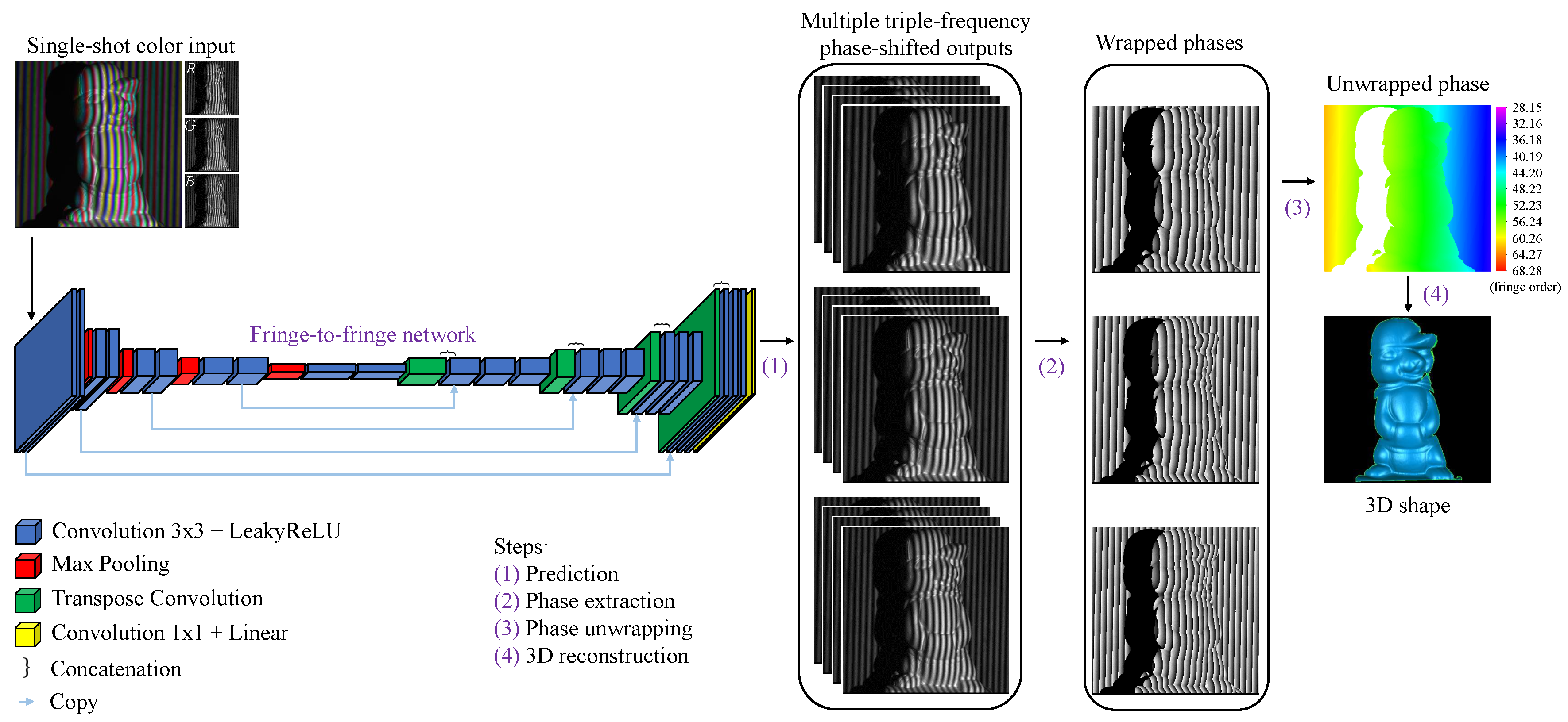
Accurate 3D Shape Reconstruction from Single Structured-Light Image via Fringe-to-Fringe Network

1
Department of Mechanical Engineering, The Catholic University of America, Washington, DC 20064, USA
2
Neuroimaging Research Branch, National Institute on Drug Abuse, National Institutes of Health, Baltimore, MD 21224, USA
*
Author to whom correspondence should be addressed.
Photonics 2021, 8(11), 459; https://doi.org/10.3390/photonics8110459
Submission received: 16 August 2021 / Revised: 4 October 2021 / Accepted: 18 October 2021 / Published: 20 October 2021
(This article belongs to the Special Issue Optical Sensing)

Abstract

:
Accurate three-dimensional (3D) shape reconstruction of objects from a single image is a challenging task, yet it is highly demanded by numerous applications. This paper presents a novel 3D shape reconstruction technique integrating a high-accuracy structured-light method with a deep neural network learning scheme. The proposed approach employs a convolutional neural network (CNN) to transform a color structured-light fringe image into multiple triple-frequency phase-shifted grayscale fringe images, from which the 3D shape can be accurately reconstructed. The robustness of the proposed technique is verified, and it can be a promising 3D imaging tool in future scientific and industrial applications.

1. Introduction

Three-dimensional (3D) shape or depth perception has been a favored long-term research topic in recent decades, driven by numerous scientific and engineering applications in many fields, due to its capability of perceiving depth information that cannot be fulfilled by two-dimensional (2D) imaging. The 3D shape and depth perception techniques are typically stereo vision- and optics-based, and the most widely used scheme involves employing structured light to facilitate image analysis. Representative commercial products in this category include industrial 3D scanners that provide accurate 3D shape measurements with fringe-pattern illumination and consumer-grade 3D depth sensors that deliver real-time depth maps with speckle-pattern or similar illuminations [1,2,3,4,5,6]. A fringe pattern-based technique generally requires capturing multiple fringe-shifted images in sequence to achieve high accuracy, but the measurement speed is consequently slow. By contrast, a speckle pattern-based technique usually uses two images simultaneously captured by two cameras; in this way, real-time measurement speed can be attained, but the corresponding accuracy is often relatively low. Therefore, a structured-light technique capable of providing not only high-accuracy but also fast-speed performance is always of great interest in the research and development of new 3D scanning systems.
In recent years, deep learning has seen explosive growth in an enormous range of challenging computer vision applications [7,8,9,10,11,12]. In particular, deep learning has been playing an important role in enhancing the capabilities of various 3D imaging and shape reconstruction techniques via using supervised learning and massive datasets [13,14,15,16]. In the meantime, several artificial neural networks have been successfully utilized in optical measurement applications such as fringe analysis, phase determination, interferogram denoising, and deformation investigation [17,18,19,20,21,22,23,24].
Based on the successful applications of deep learning in the computer vision and optics fields, integrating the structured-light technique and the deep learning scheme for accurate 3D shape reconstruction should be achievable [25,26,27]. As a matter of fact, a few strategies have been proposed to transform a captured structured-light image into its corresponding 3D shape using deep learning. For instance, an autoencoder-based network named UNet can serve as an end-to-end network to acquire the depth map from a single structured-light image [28,29,30,31]. Works presented in [32,33,34,35,36] reveal that a phase map can be retrieved by one or multiple neural networks from structured-light images, and the phase map is then used to calculate the depth map.
In this paper, a novel technique of 3D shape reconstruction from a single structured-light fringe image is proposed. It is based on using a high-accuracy 3D imaging technique known as fringe projection profilometry (FPP). The conventional FPP technique involves using a projector to project a set of phase-shifted fringe patterns with multiple frequencies on the target, where the surface height or depth information is naturally encoded into the images captured by a camera at a different view from the projector. Through retrieving phase distributions from the captured images, the height or depth map can be determined and the 3D shape can be reconstructed. Inspired by Zhang’s work [37] of encoding three fringe patterns of different frequencies into a single composite RGB image and a few other researchers’ work [38,39] of using a deep learning method to transform one or two fringe images to multiple phase-shifted fringe images, the proposed technique aims to employ a convolutional neural network (CNN) model to transform a single-shot red–green–blue (RGB) fringe-pattern image into a number of multi-frequency phase-shifted grayscale fringe-pattern images, which are then used to reconstruct the depth and 3D shape map using the conventional FPP algorithm. Due to the main purpose of transforming a single fringe pattern into multiple fringe patterns, the CNN model is called a fringe-to-fringe network. Compared with the conventional FPP technique, the essential difference is that the proposed approach requires only a single-shot color image instead of multiple (e.g., 12–20) images. Since the new technique requires only a single-shot image instead of multiple images, the measurement speed can be remarkably improved while maintaining equivalent accuracy. Such a highly demanded capability is technically impossible from the conventional perspective, but is now practicable with a CNN approach.
It is noteworthy that, unlike Yu’s work [38], which uses multiple networks and one or multiple fringe images, the proposed technique uses a single network and a single image for fringe-to-fringe transformations. In addition, a favorable UNet-like network other than a simple autoencoder-like network is employed to enhance the transformation performance. Furthermore, it can deal with background fringes. More importantly, by using the multiple phase-shifted fringes as an intermediary, the proposed approach achieves substantially higher accuracy than the direct transformation from fringe to depth using deep learning. Figure 1 demonstrates the fringe-to-fringe network architecture and the pipeline of the proposed approach.

2. Materials and Methods

The key step of the proposed technique is to employ a CNN model to transform a single-shot RGB fringe-pattern image into a number of phase-shifted grayscale fringe-pattern images, which are then used to reconstruct the depth and 3D shape map using the conventional FPP algorithm.
The required training and validation datasets, including input images and their corresponding fringe-pattern outputs, are generated by a conventional FPP system. The test dataset is generated in this way as well for assessment purposes. Details of the FPP technique can be found in Ref. [40]. In this work, however, to cope with the essential phase unwrapping issue, a four-step triple-frequency phase-shifting (TFPS) scheme is adopted for high-accuracy phase determination. Figure 2 exhibits the schematic pipeline of the employed conventional FPP technique, which is elaborated as follows.
The initial fringe patterns fed into the projector are evenly spaced vertical sinusoidal fringes, which are numerically generated with the following function [41]:
I i n ( p ) ( u , v ) = I 0 ( p ) 1 + c o s ϕ i ( u , v ) + δ n
where I ( p ) is the intensity of the initial pattern at the pixel coordinate ( u , v ) ; the subscript i indicates the ith frequency with i = 1 , 2 , 3 and n denotes the nth phase-shifted image with n = 1 , 2 , 3 , 4 ; I 0 ( p ) is a constant coefficient indicating the value of intensity modulation (e.g., I 0 ( p ) = 255 2 ); δ is the phase-shift amount with δ n = ( n 1 ) π 2 ; and ϕ is the fringe phase. For vertical fringes, ϕ is independent of the vertical coordinates and can be simply defined as ϕ i ( u , v ) = ϕ i ( u ) = 2 π f i u W , where f i is the number of fringes in the ith frequency pattern and W is the width of the generated image.
The fringes in the captured images are often distorted, following the 3D shapes of the targets. The fringe patterns can be described as:
I i n ( u , v ) = A i ( u , v ) + B i ( u , v ) c o s ϕ i ( u , v ) + δ n
where A, B, and I are the background intensity, fringe amplitude, and pixel intensity of the captured fringe image at pixel coordinate ( u , v ) , respectively. The phase distribution ϕ i ( u , v ) in the captured images is now a function of both u and v, and it can be determined by using a standard four-step phase-shifting scheme as:
ϕ i w ( u , v ) = arctan I i 4 ( u , v ) I i 2 ( u , v ) I i 1 ( u , v ) I i 3 ( u , v ) ,
where superscript w signifies a wrapped phase because of the arc-tangent function. ( u , v ) will be omitted hereafter for simplicity.
If the three frequencies satisfy ( f 3 f 2 ) ( f 2 f 1 ) = 1 , where ( f 3 f 2 ) > ( f 2 f 1 ) > 0 , the unwrapped phase of the highest-frequency fringe patterns can be calculated with the following hierarchical equations:
ϕ 12 w = ϕ 2 w ϕ 1 w + 2 π ϕ 1 w ϕ 2 w 0
ϕ 23 w = ϕ 3 w ϕ 2 w + 2 π ϕ 2 w ϕ 3 w 0
ϕ 123 = ϕ 23 w ϕ 12 w + 2 π ϕ 12 w ϕ 23 w 0
ϕ 23 = ϕ 23 w + INT ϕ 123 ( f 3 f 2 ) ϕ 23 w 2 π 2 π
ϕ = ϕ 3 = ϕ 3 w + INT ϕ 23 f 3 f 3 f 2 ϕ 3 w 2 π 2 π
In the equations, x 0 denotes a singularity function, and it is 1 for x 0 and is 0 otherwise; INT indicates rounding to the nearest integer. The rationale of the algorithm is to generate an intermediate result of unwrapped phase ϕ 123 to start a hierarchical phase-unwrapping process. ϕ 12 w and ϕ 23 w are intermediate wrapped phases with ( f 2 f 1 ) and ( f 3 f 2 ) fringes in the pattern, respectively. ϕ 123 is both wrapped and unwrapped because there is only one fringe in the pattern since ( f 3 f 2 ) ( f 2 f 1 ) = 1 . ϕ 23 is an intermediate unwrapped phase to bridge ϕ 123 and ϕ 3 because the ratio of their fringe numbers is large. The phase distribution of the highest-frequency fringe patterns, ϕ 3 , is adopted because it yields the highest accuracy for phase determination. In this work, the three frequencies are 61, 70, and 80. This combination gives a ratio of 1:10:80 for a balanced hierarchical calculation.
From the retrieved phase distribution, the depth map can be calculated [40] from:
z w = C p 1 p 2 D p 1 p 2 C = 1 c 1 c 2 c 3 c 17 c 18 c 19 D = d 0 d 1 d 2 d 3 d 17 d 18 d 19 p 1 = 1 ϕ u u ϕ v v ϕ u 2 u 2 ϕ u v u v ϕ v 2 v 2 ϕ p 2 = u 3 u 3 ϕ u 2 v u 2 v ϕ u v 2 u v 2 ϕ v 3 v 3 ϕ
where z w is the physical height or depth at the point corresponding to the pixel ( u , v ) in the captured image, and it is also the z-coordinate of the point in the reference world coordinate system; ϕ is the unwrapped phase of the highest-frequency fringe pattern at the same pixel, which is determined from Equation (Section 2); c 1 c 19 and d 0 d 19 are 39 constant coefficients that can be pre-determined by a calibration process [40,42]. Following this, the other two coordinates x w and y w can be easily determined upon knowing the camera parameters [42]. For this reason, the two terms, depth (or height) measurement and 3D shape reconstruction, can often be used interchangeably.
In the dataset generation, three original uniform fringe patterns with different frequencies (i.e., 61, 70, and 80) are respectively loaded into the RGB channels of the first projection image, and the following 12 projection images are the four-step TFPS grayscale images of the aforementioned three fringe patterns. For each sample, the system projects these 13 patterns onto the target and meanwhile captures 13 corresponding images. The first captured color image serves as the fringe pattern input, and the remaining 12 grayscale images aim to generate the corresponding ground-truth labels as previously described. Dozens of small plaster sculptures are randomly oriented and positioned many times in the field of view of the capturing system to serve as a large number of different samples. In total, 1500 data samples are acquired. To ensure reliable network convergence and avoid biased evaluation, the samples are split by a ratio of 80%–10%–10% as the training, validation, and test datasets. Notably, a number of objects are captured solely for the validation and test datasets to ensure that a target, regardless of rotation and position, will appear only in one of the three datasets.
Figure 3a shows a few selected input and output pairs contained in the datasets of the fringe-to-fringe network. Because a performance comparison of the proposed network with the existing fringe-to-depth and speckle-to-depth networks will be conducted later, a few examples of these two network datasets are presented in Figure 3b,c, respectively. Furthermore, since the wrapped phase can be obtained from the numerator (N) and denominator (D) of the arctangent function shown in Equation (3), a network capable of determining Ns and Ds of the captured fringe images can be suitable for the 3D shape reconstruction [43]. Such a fringe-to-ND network will also be included in the comparisons with the proposed fringe-to-fringe network. The examples of the input and output data of the fringe-to-ND network are shown in Figure 3d.
In the proposed approach, a UNet-based CNN network [11] is constructed for the fringe-to-fringe transformation. In particular, the CNN model is trained to transform each fringe pattern in the RGB channels of the input image into its corresponding four-step phase-shifted fringe images. The appearance of the target and background remain the same in the output images, and the only change is the shifting of the fringe patterns at an incremental step of π 2 . The network consists of two main paths: an encoder path and a decoder path. The encoder path contains spatial convolution (kernel size of 3 × 3 ) and max-pooling (pool size 2 × 2 ) layers to extract representative features from the single-shot input image, whereas the decoder path reverses the operations of the encoder path with transposed convolution (strides = 2) and spatial convolution layers to upsample the previous feature map to a higher-resolution receptive map. It is noted that all the spatial convolution and transposed convolution layers use the same padding type, in which the output feature maps have exactly the same spatial resolution as the input feature maps. In addition, symmetric concatenations from the encoder path to the decoder path are established to ensure rigorous transformation of features at different sub-scale resolutions. Finally, a 1×1 convolution layer is attached to the last layer to transform the vector feature maps into the desired fringe-pattern outputs.
The format of the training, validation, and test data, as well as the output data, is a four-dimensional (4D) tensor of size s × h × w × c , where the four variables are the number of data samples, the height and width of input and output images, and the channel depth, respectively. Specifically, h and w are 352 and 640, respectively; c is set to 3 for the RGB input image and 12 for the output of multiple phase-shifted grayscale fringe images. The adopted resolution of the images is restricted by the computation system. In the network model, a dropout function with a rate of 0.2 is added to the network to prevent the overfitting issue. In addition, a nonlinear activation function named the leaky rectified linear unit (LeakyReLU) [44] is applied after each spatial convolution layer in the network to handle the zero-gradient issue. The LeakyReLU function is expressed:
h = g ( W x + b ) = W x i f W x > 0 α W x e l s e
where x and h are the input and output vectors, respectively; weight parameters W in matrix form and bias parameters b in vector form are optimized by the training process; and α is a negative slope coefficient, which is set to 0.2 in the proposed work. Table 1 details the architecture and the number of parameters of the proposed network for fringe-to-fringe transformation.

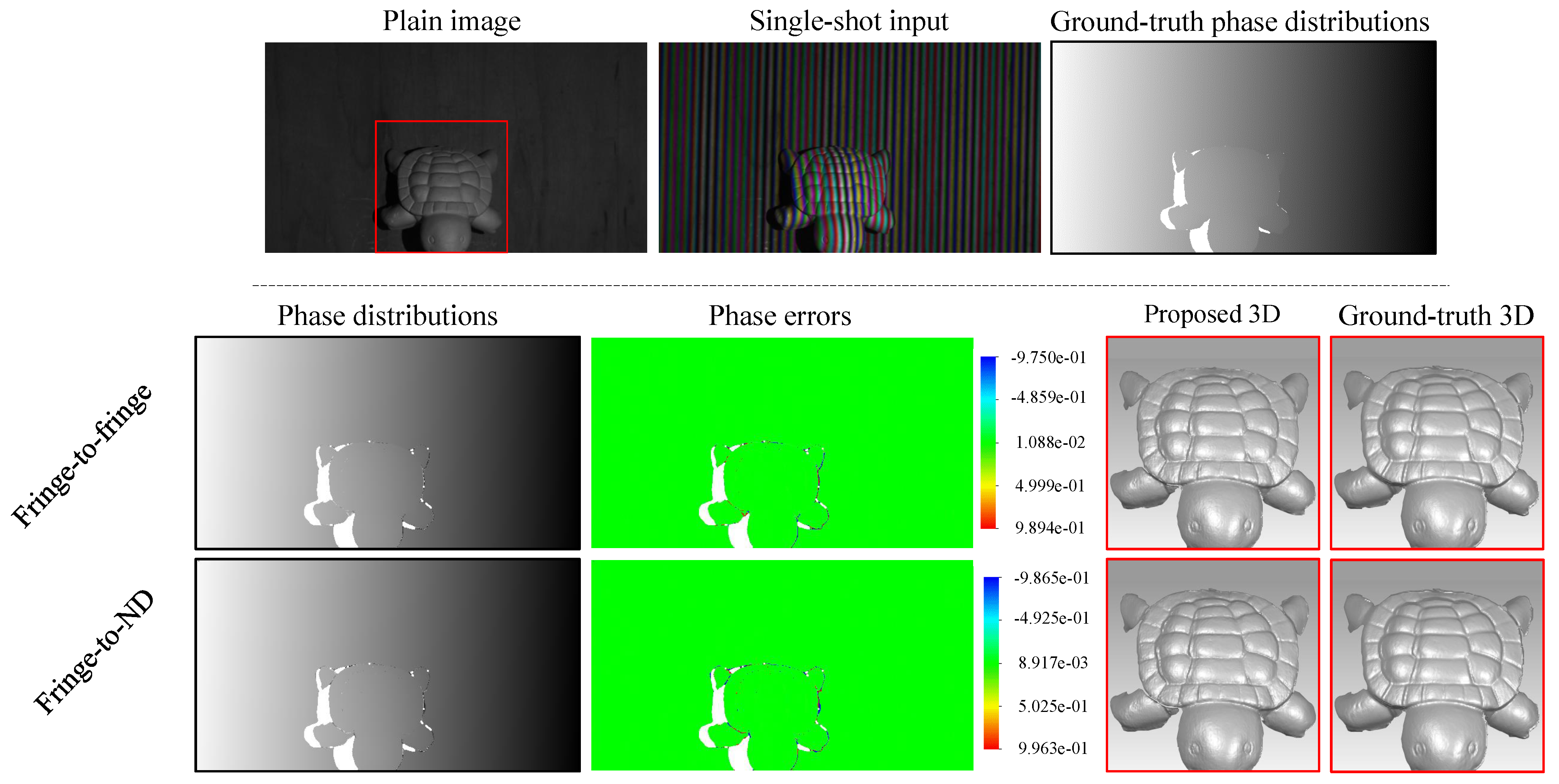
3. Results and Discussion

The hardware components used for the training process consist of an Intel Xeon Gold 6140 2.3GHz CPU, 128GB RAM, and two Nvidia Tesla V100 SXM2 32GB graphics cards. Furthermore, Nvidia CUDA Toolkit 11.0 and cuDNN v8.0.3 are adopted to enable the high-performance computing capability of the GPU. Tensorflow and Keras, two widely used open-source software libraries for deep learning, are chosen in this work for network construction and subsequent learning tasks. The datasets are captured by an RVBUST RVC-X mini 3D camera that allows the capturing of the required fringe-pattern images and the use of user-defined functions to determine 3D shapes.
For reliable and efficient performance, both the model parameters and the hyperparameters that control the learning process are optimized during training. The network is trained through 300 epochs with a mini-batch size of 2. Adam optimization [45] with a step decay schedule is implemented to gradually reduce the initial learning rate (0.0001) after the first 150 epochs. A data augmentation scheme (e.g., whitening) is implemented to overcome the modulation overfitting problem. A few Keras built-in functions such as ModelCheckpoint and LambdaCallback are applied to monitor the training performance and save the model parameters that yield the best results.
After the training is completed, the test datasets are fed into the trained CNN model to obtain the output fringe images. These images are then analyzed following Equations (3)–(5) to reconstruct the depth map and subsequent 3D shapes. Table 2 summarizes a few quantitative statistical metrics from the test dataset as well as the validation dataset. The metrics include root-mean-square error (RMSE), mean error, median error, trimean error, mean of the best 25%, and mean of the worst 25%. Because using an end-to-end neural network to directly transform a single-shot fringe or speckle image into its corresponding 3D shape or depth map has most recently gained a great deal of interest [46,47], a comparison with such a fringe-to-depth network and a speckle-to-depth network is conducted. Moreover, a fringe-to-ND network [32,34,43,48] is carried out for comparison as well since it is an approach falling between the fringe-to-depth and the proposed fringe-to-fringe network. The comparative work uses the same system configuration as well as network architecture shown in Figure 1. For the fringe-to-depth network, the difference from the proposed fringe-to-fringe one is that the channel depth of the last convolution layer is changed from 12 to 1 to accommodate the depth map requirement (i.e., c = 1 ). For the speckle-to-depth network, the channel depth of the input is one instead of three since the speckle image is grayscale. For the fringe-to-ND network, the channel depth of the output is six because there are three numerator maps and three denominator maps. The results displayed in the table clearly show that the proposed technique works well and outperforms the fringe-to-depth network and the speckle-to-depth network methods. It also performs slightly better than the fringe-to-ND network scheme.
Figure 4 displays the 3D results of the proposed approach with the fringe-to-fringe network and the comparative fringe-to-depth network. In the figure, the first to fifth rows are the plain images, the test inputs, followed by the 3D labels, the 3D shapes obtained from the fringe-to-fringe network, and the results from the fringe-to-depth network, respectively. For each of the two sample objects, a selected feature region is magnified for better comparison purposes. It is evident that the proposed approach with the fringe-to-fringe network is capable of acquiring 3D results with detailed textures close to the ground-truth labels, whereas the technique with the direct fringe-to-depth network reconstructs the 3D shape of the target with fewer details and larger errors.
Figure 5 demonstrates a qualitative comparison assessment between the proposed fringe-to-fringe approach and the recently developed speckle-to-depth method. The top portion of the figure shows the fringe-pattern input and speckle-pattern input required by the fringe-to-fringe and speckle-to-depth methods, respectively. From the shape reconstruction results displayed in the bottom portion of the figure, it is evident that the speckle-to-depth scheme reconstructs fewer surface details than the proposed fringe-to-fringe approach.
To further illustrate the performance of the proposed approach, Figure 6 shows the results of another two representative test samples. The first column in the top portion of the figure displays the single-shot inputs, and the next two columns are the phase distributions retrieved from the predicted fringe patterns and their ground truth. The first two columns in the bottom portion of the figure are the phase differences between the predicted and ground-truth ones. The last two columns demonstrate the 3D shapes reconstructed by the proposed technique and the conventional structured-light FPP technique. The mean values of the phase differences obtained for the two test samples are 2.616 × 10 4 and 3.958 × 10 4 , respectively. It can be seen again that the proposed technique can reconstruct high-quality 3D shapes comparable to the ones reconstructed by the state-of-the-art structured-light technique, except for some noise along the edges.
Figure 7 exhibits a comparative demonstration of the proposed fringe-to-fringe approach and the fringe-to-ND method. The first row of the figure includes the plain image, fringe-pattern input, and ground-truth unwrapped phase distributions. The second and third rows plot the unwrapped phase distributions obtained from the predicted outputs, phase errors, and 3D shapes reconstructed by the fringe-to-fringe and fringe-to-ND methods. It is observed that both techniques can acquire 3D shapes close to the 3D ground-truth label, with detailed surface information. Nevertheless, a closer inspection reveals that the fringe-to-fringe technique can provide slightly better results than the fringe-to-ND approach. The performance has been reflected in Table 2 previously presented.
The last experiment is accomplished to demonstrate the practicality of the proposed technique for the 3D shape reconstruction of multiple separated objects. Conventionally, such a task involving geometric discontinuities cannot be fulfilled by an automated single-shot fringe-projection-based technique due to the ambiguity in determining discontinuous fringe orders. Nevertheless, the discontinuity of fringe orders can be identified by the proposed network since it produces multiple TFPS fringe patterns. This can be observed in Figure 8.

4. Conclusions

In summary, a novel, accurate single-shot 3D shape reconstruction technique integrating the structured-light technique and deep learning is presented. The proposed fringe-to-fringe network transforms a single RGB color fringe pattern into multiple phase-shifted grayscale fringe patterns demanded by the subsequent 3D shape reconstruction process. The characteristics of single-shot input can help to substantially reduce the capturing time; meanwhile, the accuracy can be maintained since the final 3D reconstruction is based on the conventional state-of-the-art high-accuracy algorithm.
The conventional structured-light-based FPP technique consists of a few temporal steps to decode the fringe patterns and reconstruct the 3D shapes. Any of the intermediate data, including phase-shifted patterns, wrapped phase distributions, fringe orders, unwrapped phase distributions, and height maps, may serve as the output in a deep learning network for the 3D shape reconstruction. In other words, the deep learning approach may be applied to any stage of the conventional FPP technique to facilitate the analysis and processing. Technically, a direct and straightforward 2D-to-3D conversion technique such as the fringe-to-depth method is desired. However, the complex relations between a camera-captured 2D image and its corresponding 3D shapes make such a direct transformation challenging when high-accuracy reconstruction is demanded. The experimental results presented in this paper show that the performance of the proposed approach is superior to that of other deep-learning-based methods. The proposed fringe-to-fringe technique uses the predicted multiple phase-shifted patterns as an intermediary to bridge a single 2D image and its corresponding 3D shape. It benefits from the fact that the relation of the single-shot input with the predicted fringe patterns is less complex than its relation with other intermediate results.
Because RGB color images are used in the proposed technique, it is generally not suitable for working with objects of dark colors, particularly vivid red, green, and blue colors. This is a limitation of the proposed technique. In the meantime, it should be pointed out that the projector and camera were initially color-calibrated by the manufacturers, and no special handling was applied to deal with the color cross-talk. The experimental results have shown that the inevitable minor color cross-talk can be handled well by the technique.
The real-time and high-accuracy 3D shape reconstruction capability of the proposed approach provides a great solution for future scientific research and industrial applications.

Author Contributions

Conceptualization, H.N. and Z.W.; methodology, H.N. and Z.W.; software, H.N. and Z.W.; validation, H.N.; formal analysis, H.N.; investigation, H.N. and Z.W.; data curation, H.N.; writing—original draft preparation, H.N.; writing—review and editing, Z.W.; visualization, H.N. and Z.W.; supervision, Z.W. All authors have read and agreed to the published version of the manuscript.

Funding

This research received no external funding.

Data Availability Statement

The data presented in this study are available on request from the corresponding author. The data are not publicly available due to confidentiality agreements and ethical concerns.

Acknowledgments

This work utilized the computational resources of the NIH HPC Biowulf cluster (http://hpc.nih.gov (accessed on 17 October 2021)).

Conflicts of Interest

The authors declare no conflict of interest.

References

  1. Khoshelham, K.; Elberink, S.O. Accuracy and resolution of Kinect depth data for indoor mapping applications. Sensors 2012, 12, 1437–1454. [Google Scholar] [CrossRef] [Green Version]
  2. Xu, J.; Zhang, S. Status, challenges, and future perspectives of fringe projection profilometry. Opt. Lasers Eng. 2020, 135, 106193. [Google Scholar] [CrossRef]
  3. Keselman, L.; Woodfill, J.I.; Grunnet-Jepsen, A.; Bhowmik, A. Intel(R) RealSense(TM) Stereoscopic Depth Cameras. In Proceedings of the IEEE Conference on Computer Vision and Pattern Recognition Workshops (CVPRW), Honolulu, HI, USA, 21–26 July 2017; pp. 1267–1276. [Google Scholar] [CrossRef]
  4. Nguyen, H.; Wang, Z.; Jones, P.; Zhao, B. 3D shape, deformation, and vibration measurements using infrared Kinect sensors and digital image correlation. Appl. Opt. 2017, 56, 9030–9037. [Google Scholar] [CrossRef]
  5. ATOS Core: Precise Industrial 3D Metrology. Available online: https://www.atos-core.com/ (accessed on 4 October 2021).
  6. ZEISS colin3D-Optical 3D Capture and 3D Analysis. Available online: https://www.zeiss.com/metrology/products/software/colin3d.html (accessed on 4 October 2021).
  7. LeCun, Y.; Bengio, Y.; Hinton, G. Deep learning. Nature 2016, 521, 436–444. [Google Scholar] [CrossRef]
  8. Voulodimos, A.; Doulamis, N.; Doulamis, A.; Protopapadakis, E. Deep Learning for Computer Vision: A Brief Review. Comput. Intell. Neurosci. 2018, 2018. [Google Scholar] [CrossRef]
  9. Pathak, A.; Pandey, M.; Rautaray, S. Application of Deep Learning for Object Detection. Proced. Comp. Sci. 2018, 132, 1706–1717. [Google Scholar] [CrossRef]
  10. Bianco, V.; Mazzeo, P.; Paturzo, M.; Distante, C.; Ferraro, P. Deep learning assisted portable IR active imaging sensor spots and identifies live humans through fire. Opt. Lasers Eng. 2020, 124, 105818. [Google Scholar] [CrossRef]
  11. Ronneberger, O.; Fischer, P.; Brox, T. U-Net: Convolutional Networks for Biomedical Image Segmentation. In Medical Image Computing and Computer-Assisted Intervention; Springer: Cham, Switzerland, 2015; pp. 234–241. [Google Scholar] [CrossRef] [Green Version]
  12. Han, X.F.; Laga, H.; Bennamoun, M. Image-Based 3D Object Reconstruction: State-of-the-Art and Trends in the Deep Learning Era. IEEE Trans. Patt. Anal. Mach. Intell. 2021, 43, 1578–1604. [Google Scholar] [CrossRef] [Green Version]
  13. Chen, J.; Kira, Z.; Cho, Y. Deep Learning Approach to Point Cloud Scene Understanding for Automated Scan to 3D Reconstruction. J. Comp. Civ. Eng. 2019, 33, 105818. [Google Scholar] [CrossRef]
  14. Fanello, S.; Rhemann, C.; Tankovich, V.; Kowdle, A.; Escolano, S.; Kim, D.; Izadi, S. Hyperdepth: Learning depth from structured light without matching. In Proceedings of the IEEE Conference on Computer Vision and Pattern Recognition (CVPR), Las Vegas, NV, USA, 27–30 June 2016; pp. 5441–5450. [Google Scholar] [CrossRef]
  15. Wang, H.; Yang, J.; Liang, W.; Tong, X. Deep single-view 3d object reconstruction with visual hull embedding. In Proceedings of the AAAI Conference on Artificial Intelligence, Honolulu, HI, USA, 27 January–1 February 2019; pp. 8941–8948. [Google Scholar] [CrossRef] [Green Version]
  16. Zhu, Z.; Wang, X.; Bai, S.; Yao, C.; Bai, X. Deep Learning Representation using Autoencoder for 3D Shape Retrieval. Neurocomputing 2016, 204, 41–50. [Google Scholar] [CrossRef] [Green Version]
  17. Lin, B.; Fu, S.; Zhang, C.; Wang, F.; Li, Y. Optical fringe patterns filtering based on multi-stage convolution neural network. Opt. Lasers Eng. 2020, 126, 105853. [Google Scholar] [CrossRef] [Green Version]
  18. Yan, K.; Yu, Y.; Huang, C.; Sui, L.; Qian, K.; Asundi, A. Fringe pattern denoising based on deep learning. Opt. Comm. 2019, 437, 148–152. [Google Scholar] [CrossRef]
  19. Yuan, S.; Hu, Y.; Hao, Q.; Zhang, S. High-accuracy phase demodulation method compatible to closed fringes in a single-frame interferogram based on deep learning. Opt. Express 2021, 29, 2538–2554. [Google Scholar] [CrossRef] [PubMed]
  20. Wang, K.; Li, Y.; Kemao, Q.; Di, J.; Zhao, J. One-step robust deep learning phase unwrapping. Opt. Express 2019, 27, 15100–15115. [Google Scholar] [CrossRef]
  21. Zhang, J.; Tian, X.; Shao, J.; Luo, H.; Liang, R. Phase unwrapping in optical metrology via denoised and convolutional segmentation networks. Opt. Express 2019, 27, 14903–14912. [Google Scholar] [CrossRef] [PubMed] [Green Version]
  22. Qiao, G.; Huang, Y.; Song, Y.; Yue, H.; Liu, Y. A single-shot phase retrieval method for phase measuring deflectometry based on deep learning. Opt. Comm. 2020, 476, 126303. [Google Scholar] [CrossRef]
  23. Li, Y.; Shen, J.; Wu, Z.; Zhang, Q. Passive binary defocusing for large depth 3D measurement based on deep learning. Appl. Opt. 2021, 60, 7243–7253. [Google Scholar] [CrossRef] [PubMed]
  24. Nguyen, H.; Dunne, N.; Li, H.; Wang, Y.; Wang, Z. Real-time 3D shape measurement using 3LCD projection and deep machine learning. Appl. Opt 2019, 58, 7100–7109. [Google Scholar] [CrossRef]
  25. Liang, J.; Zhang, J.; Shao, J.; Song, B.; Yao, B.; Liang, R. Deep Convolutional Neural Network Phase Unwrapping for Fringe Projection 3D Imaging. Sensors 2020, 20, 3691. [Google Scholar] [CrossRef]
  26. Yang, T.; Zhang, Z.; Li, H.; Li, X.; Zhou, X. Single-shot phase extraction for fringe projection profilometry using deep convolutional generative adversarial network. Meas. Sci. Tech. 2020, 32, 015007. [Google Scholar] [CrossRef]
  27. Fan, S.; Liu, S.; Zhang, X.; Huang, H.; Liu, W.; Jin, P. Unsupervised deep learning for 3D reconstruction with dual-frequency fringe projection profilometry. Opt. Express 2021, 29, 32547–32567. [Google Scholar] [CrossRef] [PubMed]
  28. Wang, F.; Wang, C.; Guan, Q. Single-shot fringe projection profilometry based on deep learning and computer graphics. Opt. Express 2021, 29, 8024–8040. [Google Scholar] [CrossRef] [PubMed]
  29. Nguyen, H.; Wang, Y.; Wang, Z. Single-Shot 3D Shape Reconstruction Using Structured Light and Deep Convolutional Neural Networks. Sensors 2020, 20, 3718. [Google Scholar] [CrossRef] [PubMed]
  30. Nguyen, H.; Ly, K.L.; Tran, T.; Wang, Y.; Wang, Z. hNet: Single-shot 3D shape reconstruction using structured light and h-shaped global guidance network. Results Opt. 2021, 4, 100104. [Google Scholar] [CrossRef]
  31. Zheng, Y.; Wang, S.; Li, Q.; Li, B. Fringe projection profilometry by conducting deep learning from its digital twin. Opt. Express 2020, 28, 36568–36583. [Google Scholar] [CrossRef] [PubMed]
  32. Qian, J.; Feng, S.; Tao, T.; Han, J.; Chen, Q.; Zuo, C. Single-shot absolute 3D shape measurement with deep-learning-based color fringe projection profilometry. Opt. Lett. 2020, 45, 1842–1845. [Google Scholar] [CrossRef]
  33. Shi, J.; Zhu, X.; Wang, H.; Song, L.; Guo, Q. Label enhanced and patch based deep learning for phase retrieval from single frame fringe pattern in fringe projection 3D measurement. Opt. Express 2019, 27, 28929–28943. [Google Scholar] [CrossRef]
  34. Yao, P.; Gai, S.; Chen, Y.; Chen, W.; Da, F. A multi-code 3D measurement technique based on deep learning. Opt. Lasers Eng. 2021, 143, 106623. [Google Scholar] [CrossRef]
  35. Spoorthi, G.; Gorthi, R.; Gorthi, S. PhaseNet 2.0: Phase Unwrapping of Noisy Data Based on Deep Learning Approach. IEEE Trans. Image Process. 2020, 29, 4862–4872. [Google Scholar] [CrossRef]
  36. Qian, J.; Feng, S.; Tao, T.; Hu, Y.; Li, Y.; Chen, Q.; Zuo, C. Deep-learning-enabled geometric constraints and phase unwrapping for single-shot absolute 3D shape measurement. APL Photonics 2020, 5, 046105. [Google Scholar] [CrossRef]
  37. Zhang, Z.; Towers, D.; Towers, C. Snapshot color fringe projection for absolute three-dimensional metrology of video sequences. Appl. Opt. 2010, 49, 5947–5953. [Google Scholar] [CrossRef]
  38. Yu, H.; Chen, X.; Zhang, Z.; Zuo, C.; Zhang, Y.; Zheng, D.; Han, J. Dynamic 3-D measurement based on fringe-to-fringe transformation using deep learning. Opt. Express 2020, 28, 9405–9418. [Google Scholar] [CrossRef] [PubMed]
  39. Yang, Y.; Hou, Q.; Li, Y.; Cai, Z.; Liu, X.; Xi, J.; Peng, X. Phase error compensation based on Tree-Net using deep learning. Opt. Lasers Eng. 2021, 143, 106628. [Google Scholar] [CrossRef]
  40. Vo, M.; Wang, Z.; Pan, B.; Pan, T. Hyper-accurate flexible calibration technique for fringe-projection-based three-dimensional imaging. Opt. Express 2012, 20, 16926–16941. [Google Scholar] [CrossRef]
  41. Nguyen, H.; Nguyen, D.; Wang, Z.; Kieu, H.; Le, M. Real-time, high-accuracy 3D imaging and shape measurement. Appl. Opt. 2015, 54, A9–A17. [Google Scholar] [CrossRef]
  42. Nguyen, H.; Liang, J.; Wang, Y.; Wang, Z. Accuracy assessment of fringe projection profilometry and digital image correlation techniques for three-dimensional shape measurements. J. Phys. Photonics 2021, 3, 014004. [Google Scholar] [CrossRef]
  43. Feng, S.; Zuo, C.; Yin, W.; Gu, G.; Chen, Q. Micro deep learning profilometry for high-speed 3D surface imaging. Opt. Laser Eng. 2019, 121, 416–427. [Google Scholar] [CrossRef]
  44. Mass, A.; Hannun, A.; Ng, A. Rectifier Nonlinearities Improve Neural Network Acoustic Models. In Proceedings of the International Conference on Machine Learning (ICML), Atlanta, GA, USA, 16–21 June 2013; Volume 28, p. 1. [Google Scholar]
  45. Kingma, D.; Ba, J. Adam: A Method for Stochastic Optimization. In Proceedings of the International Conference on Learning Representations (ICLR), San Diego, CA, USA, 7–9 May 2015; p. 13. [Google Scholar]
  46. Jeught, S.; Dirckx, J. Deep neural networks for single shot structured light profilometry. Opt. Express 2019, 27, 17091–17101. [Google Scholar] [CrossRef]
  47. Nguyen, H.; Tran, T.; Wang, Y.; Wang, Z. Three-dimensional Shape Reconstruction from Single-shot Speckle Image Using Deep Convolutional Neural Networks. Opt. Laser Eng. 2021, 143, 106639. [Google Scholar] [CrossRef]
  48. Yao, P.; Gai, S.; Da, F. Coding-Net: A multi-purpose neural network for Fringe Projection Profilometry. Opt. Comm. 2021, 489, 126887. [Google Scholar] [CrossRef]
Figure 1. Pipeline of the proposed approach.
Photonics 08 00459 g001
Figure 2. Pipeline of the FPP technique with triple-frequency phase-shifting scheme.
Photonics 08 00459 g002
Figure 3. Examples of input and output data pairs contained in the: (a) fringe-to-fringe datasets; (b) fringe-to-depth datasets; (c) speckle-to-depth datasets; (d) fringe-to-ND datasets.
Photonics 08 00459 g003
Figure 4. 3D shape reconstruction of the proposed technique and the comparative fringe-to-depth method.
Photonics 08 00459 g004
Figure 5. 3D shape reconstruction of the proposed technique and the comparative speckle-to-depth method.
Photonics 08 00459 g005
Figure 6. Phase distributions, phase errors, and 3D shape reconstruction of two representative test samples.
Photonics 08 00459 g006
Figure 7. Phase distributions, phase errors, and 3D shape reconstruction of the proposed fringe-to-fringe technique and the competitive fringe-to-ND approach.
Photonics 08 00459 g007
Figure 8. 3D shape reconstruction of multiple separated objects with complex shapes.
Photonics 08 00459 g008
Table 1. The proposed fringe-to-fringe architecture and layer parameters.
LayerFiltersKernel Size/
Pool Size
StrideOutput SizeParams
input---352 × 640 × 30
conv1a + LeakyReLU
conv1b + LeakyReLU
max pool
32
32
-
3 × 3
3 × 3
2 × 2
1
1
2
352 × 640 × 32
352 × 640 × 32
176 × 320 × 32
896
9248
0
conv2a + LeakyReLU
conv2b + LeakyReLU
max pool
64
64
-
3 × 3
3 × 3
2 × 2
1
1
2
176 × 320 × 64
176 × 320 × 64
88 × 160 × 64
18,496
36,928
0
conv3a + LeakyReLU
conv3b + LeakyReLU
max pool
128
128
-
3 × 3
3 × 3
2 × 2
1
1
2
88 × 160 × 128
88 × 160 × 128
44 × 80 × 128
73,856
147,584
0
conv4a + LeakyReLU
conv4b + LeakyReLU
max pool
256
256
-
3 × 3
3 × 3
2 × 2
1
1
2
44 × 80 × 256
44 × 80 × 256
22 × 40 × 256
295,168
590,080
0
conv5a + LeakyReLU
conv5b + LeakyReLU
dropout
512
512
-
3 × 3
3 × 3
-
1
1
-
22 × 40 × 512
22 × 40 × 512
22 × 40 × 512
1,180,160
2,359,808
0
transpose conv
concat
conv6a + LeakyReLU
conv6b + LeakyReLU
256
-
256
256
3 × 3
-
3 × 3
3 × 3
2
-
1
1
44 × 80 × 256
44 × 80 × 512
44 × 80 × 256
44 × 80 × 256
1,179,904
0
1,179,904
590,080
transpose conv
concat
conv7a + LeakyReLU
conv7b + LeakyReLU
128
-
128
128
3 × 3
-
3 × 3
3 × 3
2
-
1
1
88 × 160 × 128
88 × 160 × 256
88 × 160 × 128
88 × 160 × 128
295,040
0
295,040
147,584
transpose conv
concat
conv8a + LeakyReLU
conv8b + LeakyReLU
64
-
64
64
3 × 3
-
3 × 3
3 × 3
2
-
1
1
176 × 320 × 64
176 × 320 × 128
176 × 320 × 64
176 × 320 × 64
73,792
0
73,792
36,928
transpose conv
concat
conv9a + LeakyReLU
conv9b + LeakyReLU
32
-
32
32
3 × 3
-
3 × 3
3 × 3
2
-
1
1
352 × 640 × 32
352 × 640 × 64
352 × 640 × 32
352 × 640 × 32
18,464
0
18,464
9248
conv10 + Linear121 × 11352 × 640 × 12396
Total 8,630,860
Table 2. Quantitative performance of fringe-to-fringe, fringe-to-depth, and speckle-to-depth, and fringe-to-ND networks (unit: mm).
MethodFringe-to-FringeFringe-to-DepthSpeckle-to-DepthFringe-to-ND
ValiationTestValiationTestValiationTestValiationTest
RMSE0.06500.07020.56730.63760.68010.71840.06670.0538
Mean0.00910.01090.33630.37380.31670.38380.02160.0126
Median0.00870.01050.32390.35110.30300.37290.02040.0105
Trimean0.00880.01060.33100.36220.30420.37890.02070.0108
Best 25%0.00530.00400.27900.28590.21500.25430.01530.0067
Worse 25%0.01380.01810.40800.48910.44510.52890.02970.0225
Publisher’s Note: MDPI stays neutral with regard to jurisdictional claims in published maps and institutional affiliations.

