An Improved Calibration Method to Determine the Strain Coefficient for Optical Fibre Sensing Cables


Abstract
:1. Introduction
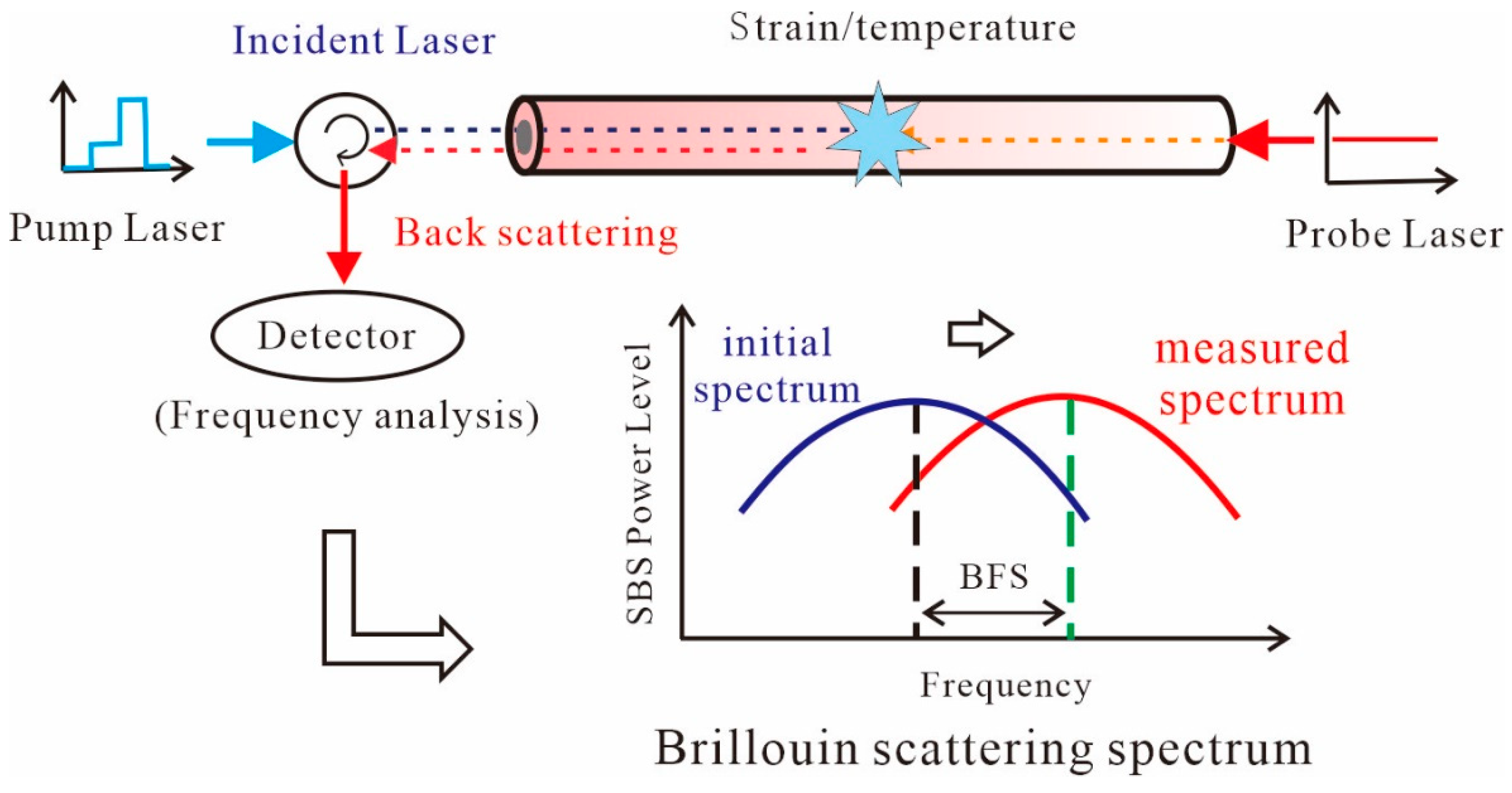
2. Principle of BOTDA
3. Materials and Methods
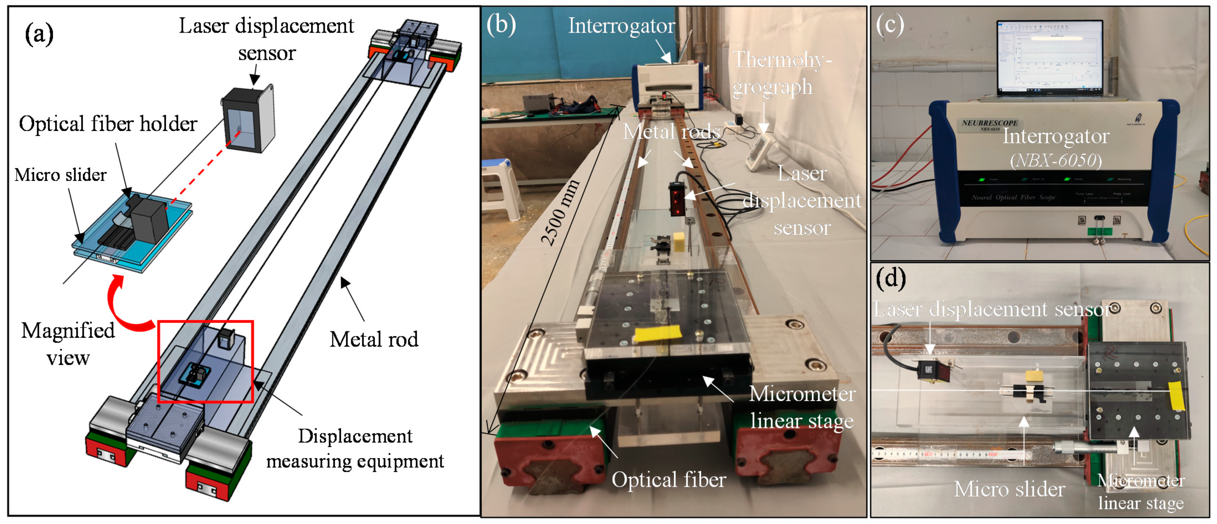
3.1. Calibration Setup
3.2. Sensing Cables
3.3. Calibration Process
4. Results and Discussion
4.1. Quality Control
4.1.1. BOTDA Interrogator
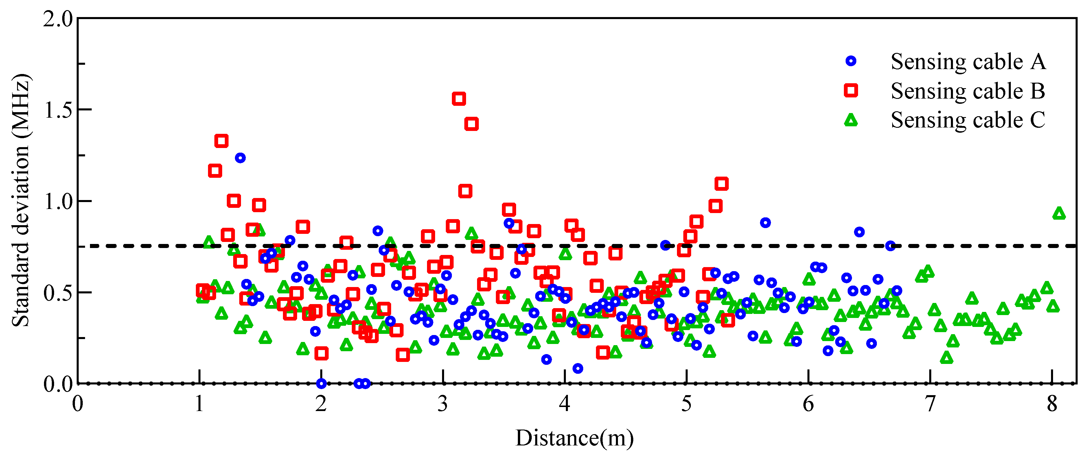
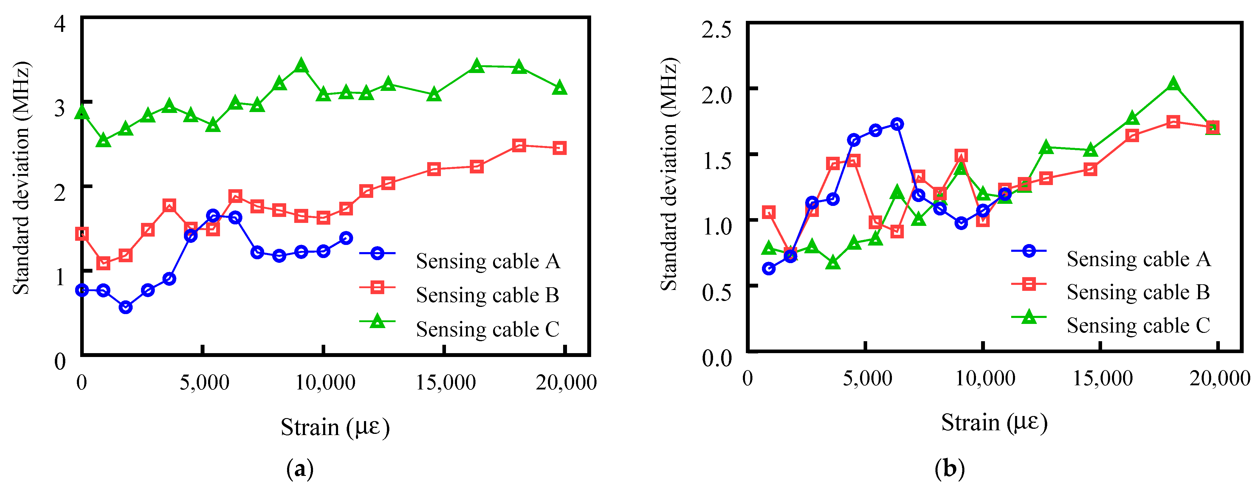
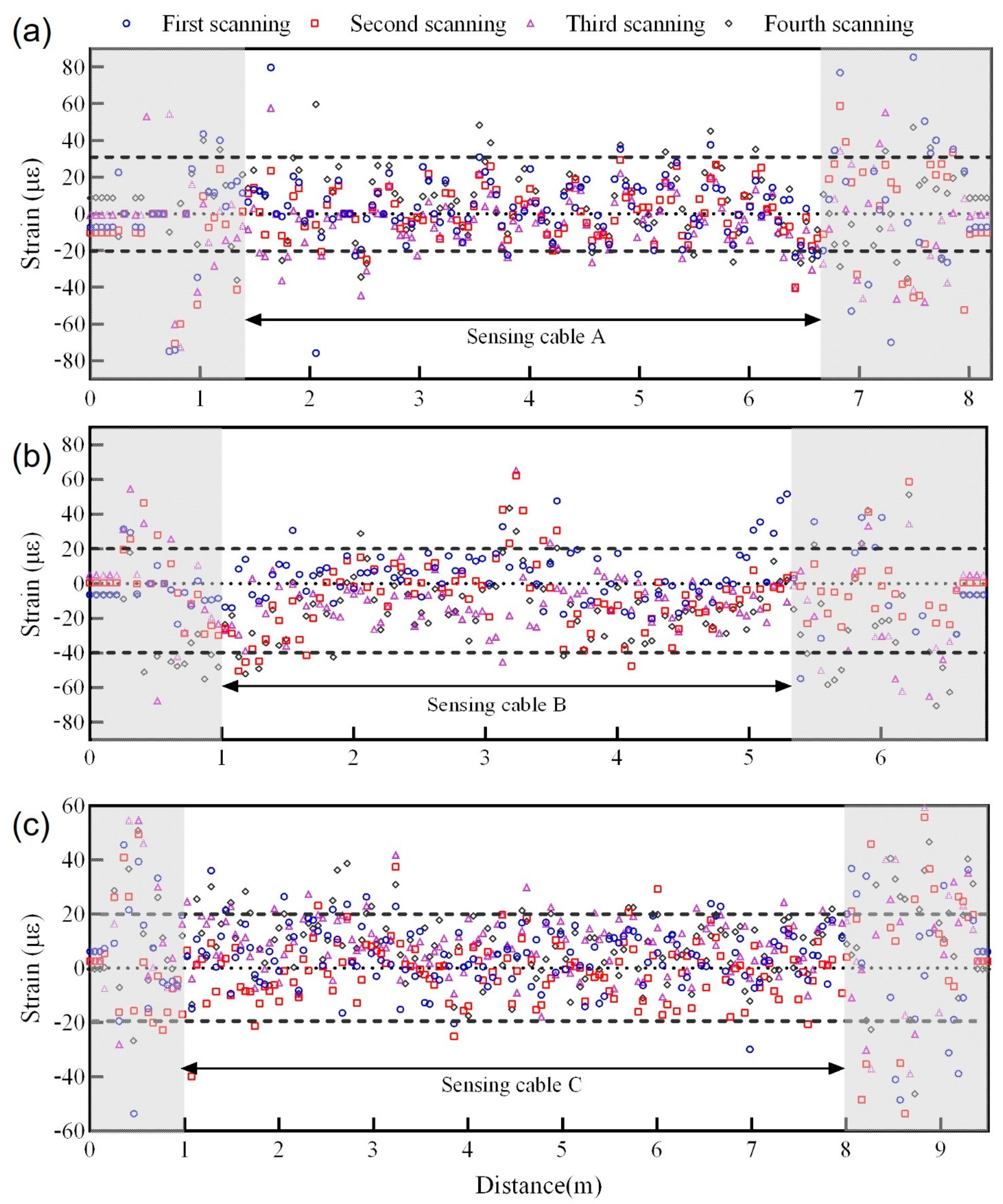
4.1.2. Uneven Strain of the Sensing Cables
4.2. Error Analysis
4.2.1. Original Length-Induced Error
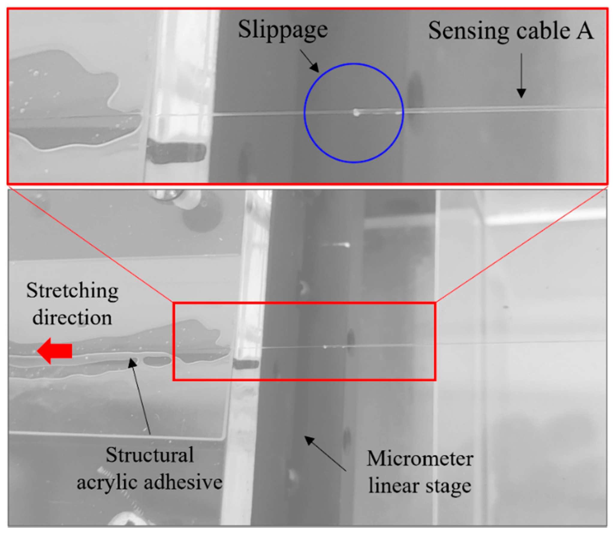
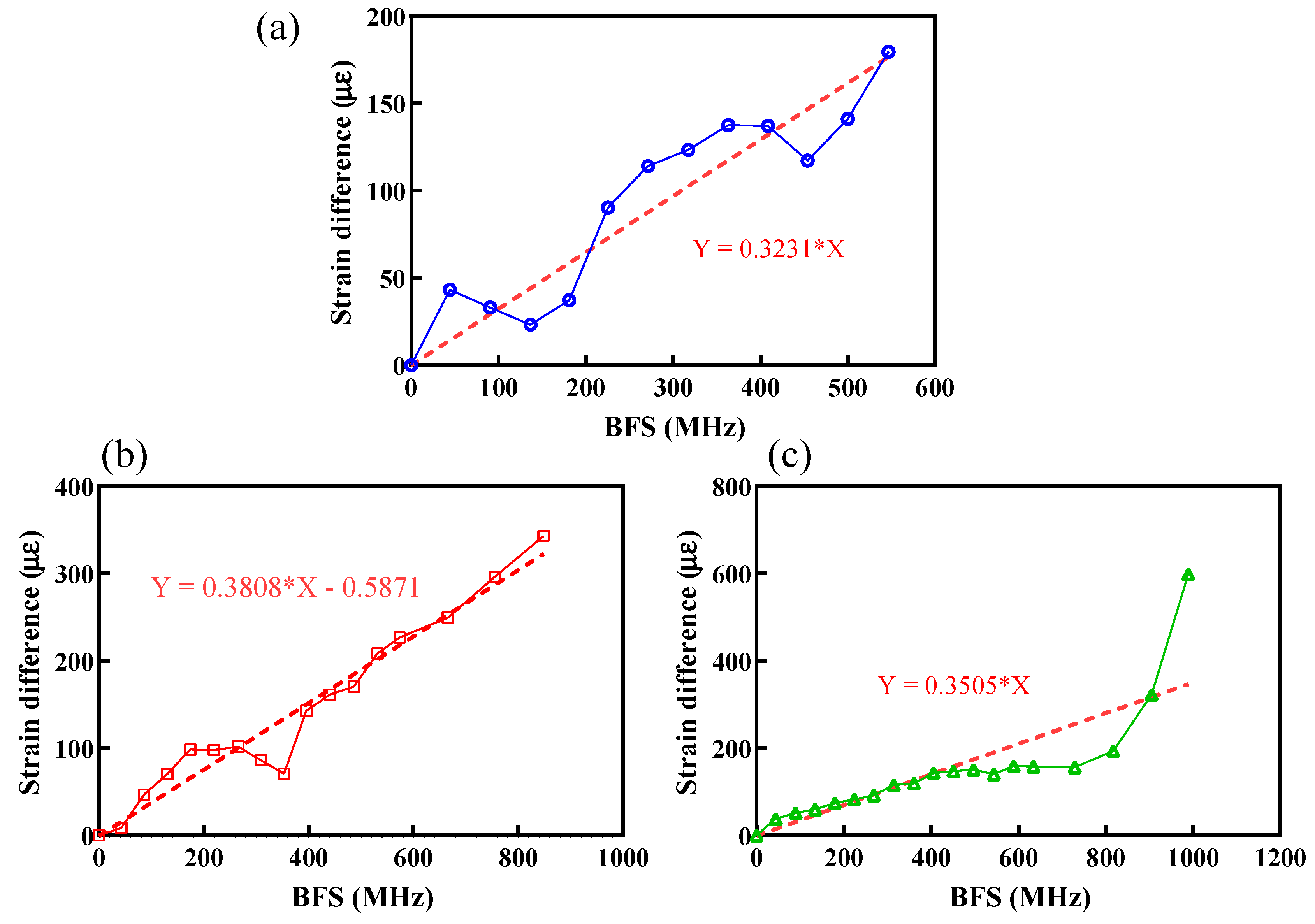
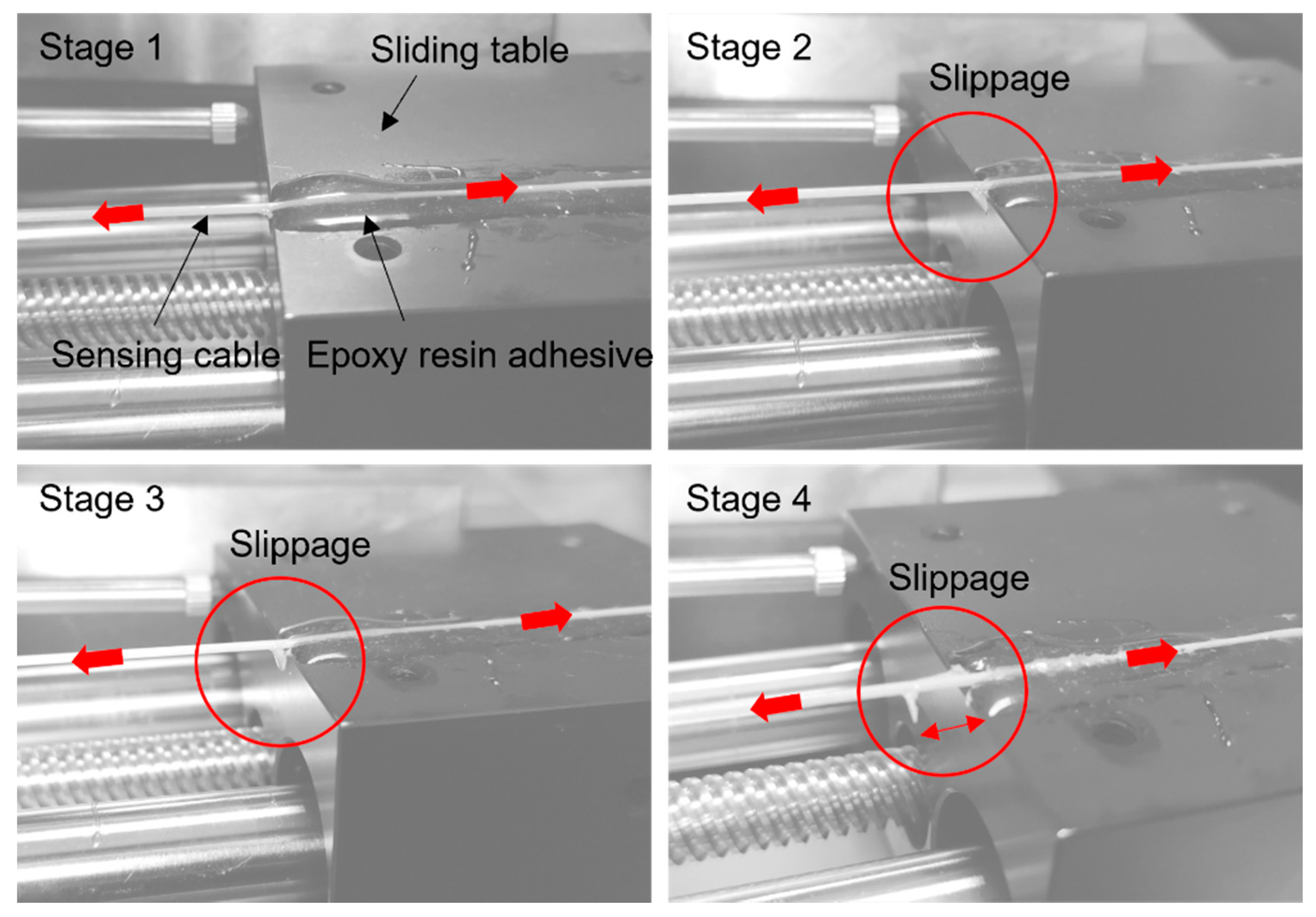
4.2.2. Slippage or Strain Transfer Loss Induced Error
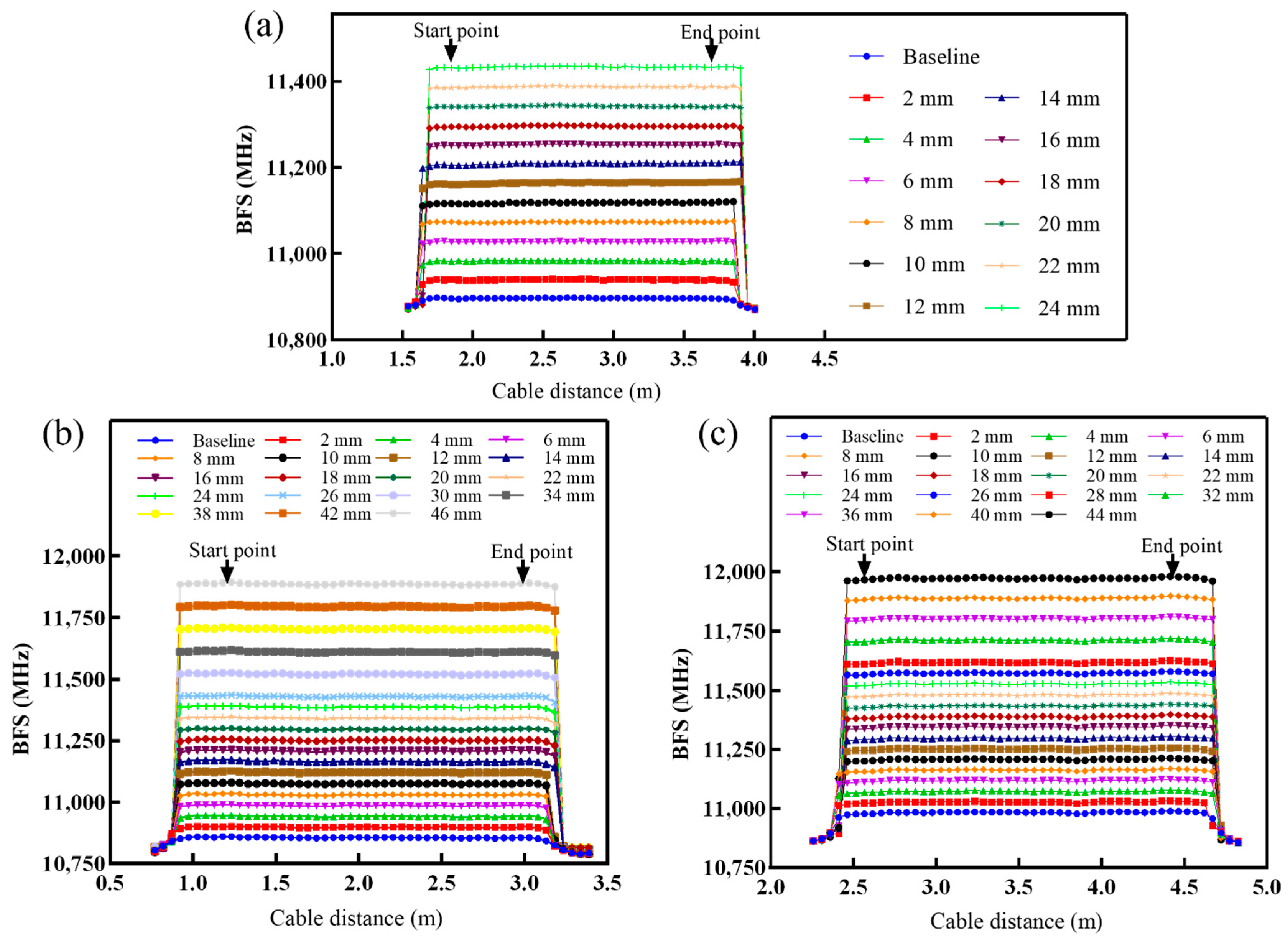
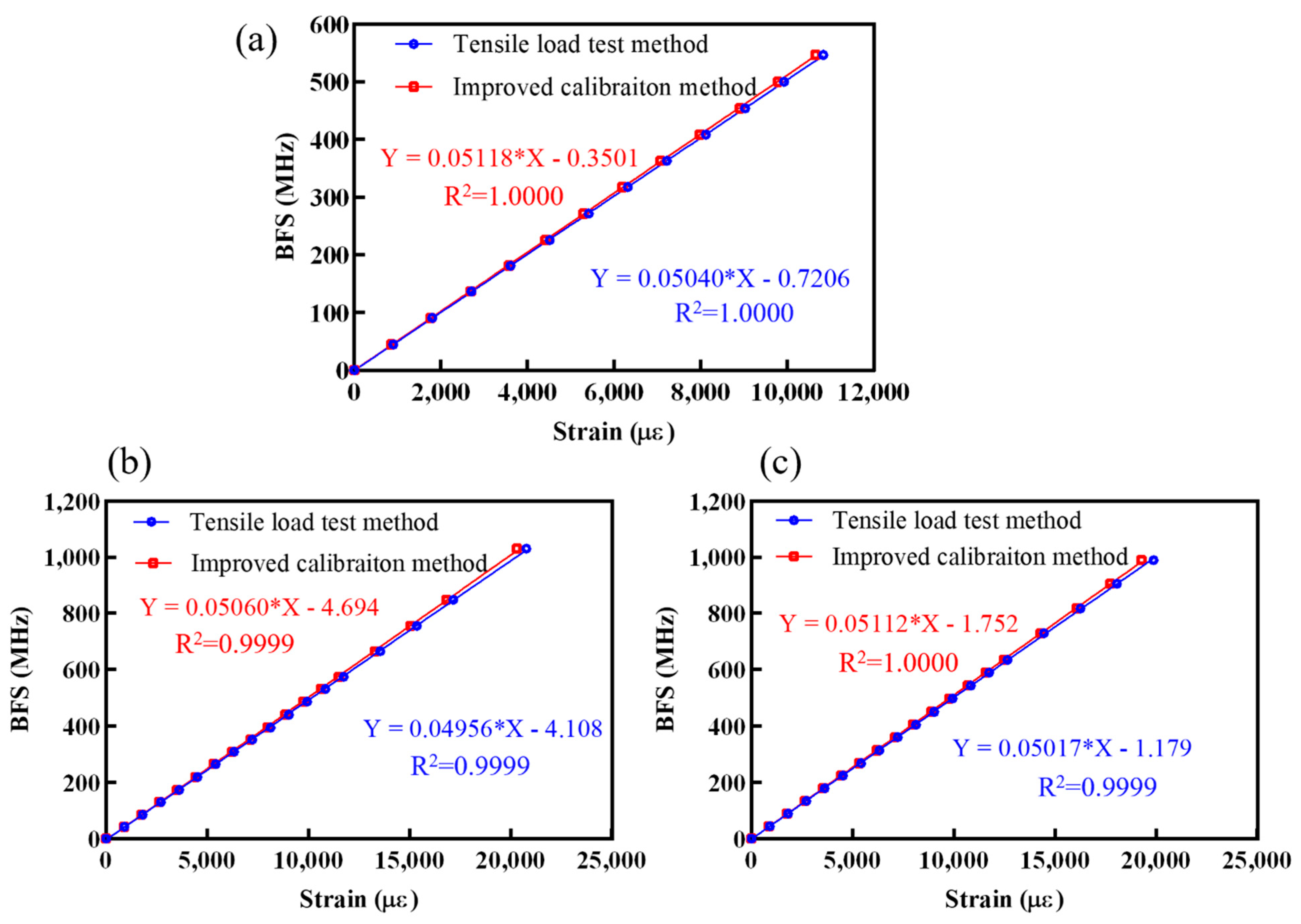
4.3. Calibration Results
4.4. The Advantages and Disadvantages of the Improved Calibration Method
5. Conclusions
- An improved strain coefficient calibration device can be developed by adding two sets of displacement measuring equipment to the traditional tensile load test setup. Thus, the strain in the mid-section of the strained sensing cable can be obtained more accurately.
- Although no slippage is observed at the fixing point in the calibration process, the results from error analysis indicate that the source of the strain coefficient calibration error is mainly due to inaccurate measurements of the displacement by the micrometre linear stage. Therefore, it can be presumed that strain transfer loss occurs between the sensing cable and micrometre linear stage.
- The performance of the improved calibration method was verified by using three types of optical fibre sensing cables. In comparison to the traditional tensile load test method, the strain coefficients obtained for sensing cables A, B, and C by using the improved calibration method are improved by 1.52%, 2.06%, and 1.86%, respectively. Although the improved calibration method only shows a slight improvement in the strain coefficient calibration results compared to the conventional tensile load test method used in this test, the improved calibration method is significant because it eliminates potential calibration errors. This enables inexperienced experimenters or facilities with limited equipment to precisely calibrate the strain coefficient of a sensing cable.
Author Contributions
Funding
Data Availability Statement
Conflicts of Interest
References
- Hong, C.-Y.; Zhang, Y.-F.; Li, G.-W.; Zhang, M.-X.; Liu, Z.-X. Recent progress of using Brillouin distributed fiber optic sensors for geotechnical health monitoring. Sens. Actuators A Phys. 2017, 258, 131–145. [Google Scholar] [CrossRef]
- Lu, P.; Lalam, N.; Badar, M.; Liu, B.; Chorpening, B.T.; Buric, M.P.; Ohodnicki, P. Distributed optical fiber sensing: Review and perspective. Appl. Phys. Rev. 2019, 6, 041302. [Google Scholar] [CrossRef]
- Bastianini, F.; Di Sante, R.; Falcetelli, F.; Marini, D.; Bolognini, G. Optical Fiber Sensing Cables for Brillouin-Based Distributed Measurements. Sensors 2019, 19, 5172. [Google Scholar] [CrossRef] [Green Version]
- Sun, Y.; Li, Q.; Yang, D.; Fan, C.; Sun, A. Investigation of the dynamic strain responses of sandstone using multichannel fiber-optic sensor arrays. Eng. Geol. 2016, 213, 1–10. [Google Scholar] [CrossRef]
- Horiguchi, T.; Kurashima, T.; Tateda, M. Tensile strain dependence of Brillouin frequency shift in silica optical fibers. IEEE Photonics Technol. Lett. 1989, 1, 107–108. [Google Scholar] [CrossRef]
- Bertholds, A.; Dandliker, R. Determination of the individual strain-optic coefficients in single-mode optical fibres. J. Light. Technol. 1988, 6, 17–20. [Google Scholar] [CrossRef]
- Hong, C.-Y.; Zhang, Y.-F.; Liu, L.-Q. Application of distributed optical fiber sensor for monitoring the mechanical performance of a driven pile. Measurement 2016, 88, 186–193. [Google Scholar] [CrossRef]
- Mendez, A.; Morse, T.; Mendez, F. Applications of Embedded Optical Fiber Sensors in Reinforced Concrete Buildings and Structures; SPIE: Bellingham, WA, USA, 1990; Volume 1170. [Google Scholar] [CrossRef]
- Mohamad, H.; Soga, K.; Bennett, P.J.; Mair, R.J.; Lim, C.S. Monitoring Twin Tunnel Interaction Using Distributed Optical Fiber Strain Measurements. J. Geotech. Geoenviron. Eng. 2012, 138, 957–967. [Google Scholar] [CrossRef]
- Su, H.; Hu, J.; Yang, M. Dam Seepage Monitoring Based on Distributed Optical Fiber Temperature System. IEEE Sens. J. 2015, 15, 9–13. [Google Scholar] [CrossRef]
- Ren, L.; Jiang, T.; Jia, Z.-G.; Li, D.-S.; Yuan, C.-L.; Li, H.-N. Pipeline corrosion and leakage monitoring based on the distributed optical fiber sensing technology. Measurement 2018, 122, 57–65. [Google Scholar] [CrossRef]
- Schenato, L.; Palmieri, L.; Camporese, M.; Bersan, S.; Cola, S.; Pasuto, A.; Galtarossa, A.; Salandin, P.; Simonini, P. Distributed optical fibre sensing for early detection of shallow landslides triggering. Sci. Rep. 2017, 7, 14686. [Google Scholar] [CrossRef]
- Barrias, A.; Casas, J.R.; Villalba, S. A Review of Distributed Optical Fiber Sensors for Civil Engineering Applications. Sensors 2016, 16, 748. [Google Scholar] [CrossRef] [PubMed] [Green Version]
- Kuang, K.S.C.; Cantwell, W.; Scully, P. An evaluation of a novel plastic optical fibre sensor for axial strain and bend measurements. Meas. Sci. Technol. 2002, 13, 1523–1534. [Google Scholar] [CrossRef]
- You, R.; Ren, L.; Song, G. A novel OFDR-based distributed optical fiber sensing tape: Design, optimization, calibration and application. Smart Mater. Struct. 2020, 29, 105017. [Google Scholar] [CrossRef]
- Her, S.-C.; Huang, C.-Y. Effect of Coating on the Strain Transfer of Optical Fiber Sensors. Sensors 2011, 11, 6926–6941. [Google Scholar] [CrossRef] [PubMed] [Green Version]
- Wan, K.T.; Leung, C.K.Y.; Olson, N.G. Investigation of the strain transfer for surface-attached optical fiber strain sensors. Smart Mater. Struct. 2008, 17, 035037. [Google Scholar] [CrossRef]
- Garcus, D.; Gogolla, T.; Krebber, K.; Schliep, F. Brillouin optical-fiber frequency-domain analysis for distributed temperature and strain measurements. J. Light. Technol. 1997, 15, 654–662. [Google Scholar] [CrossRef]
- Zaghloul, M.A.S.; Wang, M.; Milione, G.; Li, M.-J.; Li, S.; Huang, Y.-K.; Wang, T.; Chen, K.P. Discrimination of Temperature and Strain in Brillouin Optical Time Domain Analysis Using a Multicore Optical Fiber. Sensors 2018, 18, 1176. [Google Scholar] [CrossRef] [Green Version]
- Bao, Y.; Chen, G. Temperature-dependent strain and temperature sensitivities of fused silica single mode fiber sensors with pulse pre-pump Brillouin optical time domain analysis. Meas. Sci. Technol. 2016, 27, 065101. [Google Scholar] [CrossRef]
- Bo, T.; Hu, J.; Minghao, Z.; Pengfei, C.; Jiejun, L.; Xiaoyan, S. Development of Optical Fiber Strain Calibration Device. J. Phys. Conf. Ser 2020, 012097. [Google Scholar] [CrossRef]
- Delepine-Lesoille, S.; Girard, S.; Landolt, M.; Bertrand, J.; Planes, I.; Boukenter, A.; Marin, E.; Humbert, G.; Leparmentier, S.; Auguste, J.-L.; et al. France’s State of the Art Distributed Optical Fibre Sensors Qualified for the Monitoring of the French Underground Repository for High Level and Intermediate Level Long Lived Radioactive Wastes. Sensors 2017, 17, 1377. [Google Scholar] [CrossRef] [Green Version]
- Zhang, D.; Du, W.; Chai, J.; Lei, W. Strain Test Performance of Brillouin Optical Time Domain Analysis and Fiber Bragg Grating Based on Calibration Test. Sens. Mater. 2021, 33, 1387. [Google Scholar] [CrossRef]
- Chai, J.; Du, W.; Yuan, Q.; Zhang, D. Analysis of test method for physical model test of mining based on optical fiber sensing technology detection. Opt. Fiber Technol. 2019, 48, 84–94. [Google Scholar] [CrossRef]
- Kishida, K.; Yamauchi, Y.; Guzik, A. Study of optical fibers strain-temperature sensitivities using hybrid Brillouin-Rayleigh system. Photonic Sens. 2014, 4, 1–11. [Google Scholar] [CrossRef] [Green Version]
- ASTM In Standard Practice for Use of Distributed Optical Fiber Sensing Systems for Monitoring the Impact of Ground Movements during Tunnel and Utility Construction on Existing Underground Utilities; ASTM: West Conshohocken, PA, USA, 2014. [CrossRef]
- Ismail, A.; binti Siat, Q.A.; bin Kassim, A.; bin Mohamad, H. Strain and temperature calibration of Brillouin Optical Time Domain Analysis (BOTDA) sensing system. In IOP Conference Series: Materials Science and Engineering; IOP Publishing: Bristol, UK, 2019; p. 012028. [Google Scholar] [CrossRef]
- Uchida, S.; Levenberg, E.; Klar, A. On-specimen strain measurement with fiber optic distributed sensing. Measurement 2015, 60, 104–113. [Google Scholar] [CrossRef]
- Planes, I.; Girard, S.; Boukenter, A.; Marin, E.; Delepine-Lesoille, S.; Marcandella, C.; Ouerdane, Y. Steady γ-ray Effects on the Performance of PPP-BOTDA and TW-COTDR Fiber Sensing. Sensors 2017, 17, 396. [Google Scholar] [CrossRef] [Green Version]
- Falcetelli, F.; Rossi, L.; Di Sante, R.; Bolognini, G. Strain Transfer in Surface-Bonded Optical Fiber Sensors. Sensors 2020, 20, 3100. [Google Scholar] [CrossRef]
- Smith, R.G. Optical Power Handling Capacity of Low Loss Optical Fibers as Determined by Stimulated Raman and Brillouin Scattering. Appl. Opt. 1972, 11, 2489–2494. [Google Scholar] [CrossRef] [PubMed]
- Horiguchi, T.; Tateda, M. BOTDA-nondestructive measurement of single-mode optical fiber attenuation characteristics using Brillouin interaction: Theory. J. Light. Technol. 1989, 7, 1170–1176. [Google Scholar] [CrossRef]
- Zhao, M.; Yi, X.; Zhang, J.; Lin, C. PPP-BOTDA Distributed Optical Fiber Sensing Technology and Its Application to the Baishuihe Landslide. Front. Earth Sci. 2021, 9, 281. [Google Scholar] [CrossRef]
- Mohamad, H. Temperature and strain sensing techniques using Brillouin optical time domain reflectometry. In Smart Sensor Phenomena, Technology, Networks, and Systems Integration 2012; International Society for Optics and Photonics: Bellingham, WA, USA, 2012; Volume 8346. [Google Scholar] [CrossRef] [Green Version]
- An, P.; Fang, K.; Jiang, Q.; Zhang, H.; Zhang, Y. Measurement of Rock Joint Surfaces by Using Smartphone Structure from Motion (SfM) Photogrammetry. Sensors 2021, 21, 922. [Google Scholar] [CrossRef] [PubMed]


| Instrumentation | Specification | Photograph |
|---|---|---|
| Optical interrogator | Product type: NBX6050 Measurement: PPP_BOTDA Laser wavelength: 1550 nm Distance range: 50 m, 100 mm … 25 km Measurement frequency range: 9~13 GHz Range of strain measurements: −3%~+4% Strain measurement accuracy: ±15 με/0.75 °C |  |
| Metal rod | Material: bearing steel Rail Length: 2500 mm Rail width: 50 mm Weight: 21.18 kg/m Elastic modulus: 200 GPa | 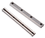 |
| Micrometre linear stage | Platform dimension: 125 mm × 125 mm Displacement range: ±12.5 mm Load: 180 N Accuracy: 0.02 mm Minimum scale: 0.01 mm Weight: 1.4 kg |  |
| Laser displacement sensor | Model: HG-C1100 Beam diameter: 0.12 mm Measuring centre distance: 100 mm Measurable range: ±35 mm Accuracy: 0.07 mm Dimension (mm): 20 × 44 × 25 |  |
| Name | Sensing Cable A | Sensing Cable B | Sensing Cable C | |
| Mode | G.652 D | G.652 D | G.652 B | |
| Optical Fibre Diameter | 250 μm | 0.9 mm | 2 mm | |
| Attenuation | 1310 nm | 0.353 dB/km | 0.330 dB/km | -- |
| 1550 nm | 0.222 dB/km | 0.185 db/km | -- | |
| Core-Cladding concentricity error | ≤0.6 μm | ≤0.6 μm | -- | |
| Manufacturer | HengTong group, Jiangsu, China | Yangtze Optical Fibre and Cable Joint Stock Limited Company, Wuhan, China | NanZee Sensing company, Nanjing, China | |
| Structure | 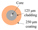 |  | 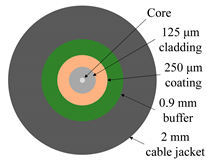 | |
| Photograph |  |  | 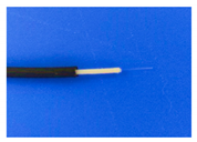 | |
Publisher’s Note: MDPI stays neutral with regard to jurisdictional claims in published maps and institutional affiliations. |
© 2021 by the authors. Licensee MDPI, Basel, Switzerland. This article is an open access article distributed under the terms and conditions of the Creative Commons Attribution (CC BY) license (https://creativecommons.org/licenses/by/4.0/).
Share and Cite
An, P.; Wei, C.; Tang, H.; Deng, Q.; Yu, B.; Fang, K. An Improved Calibration Method to Determine the Strain Coefficient for Optical Fibre Sensing Cables. Photonics 2021, 8, 429. https://doi.org/10.3390/photonics8100429
An P, Wei C, Tang H, Deng Q, Yu B, Fang K. An Improved Calibration Method to Determine the Strain Coefficient for Optical Fibre Sensing Cables. Photonics. 2021; 8(10):429. https://doi.org/10.3390/photonics8100429
Chicago/Turabian StyleAn, Pengju, Chaoqun Wei, Huiming Tang, Qinglu Deng, Bofan Yu, and Kun Fang. 2021. "An Improved Calibration Method to Determine the Strain Coefficient for Optical Fibre Sensing Cables" Photonics 8, no. 10: 429. https://doi.org/10.3390/photonics8100429
APA StyleAn, P., Wei, C., Tang, H., Deng, Q., Yu, B., & Fang, K. (2021). An Improved Calibration Method to Determine the Strain Coefficient for Optical Fibre Sensing Cables. Photonics, 8(10), 429. https://doi.org/10.3390/photonics8100429