Effective Medium Theory for Multi-Component Materials Based on Iterative Method


Abstract
1. Introduction
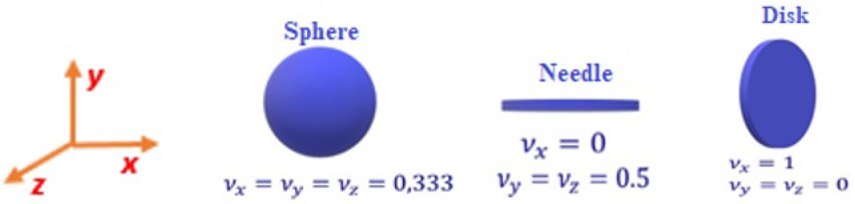
2. Basics
3. Derivation
4. Validation
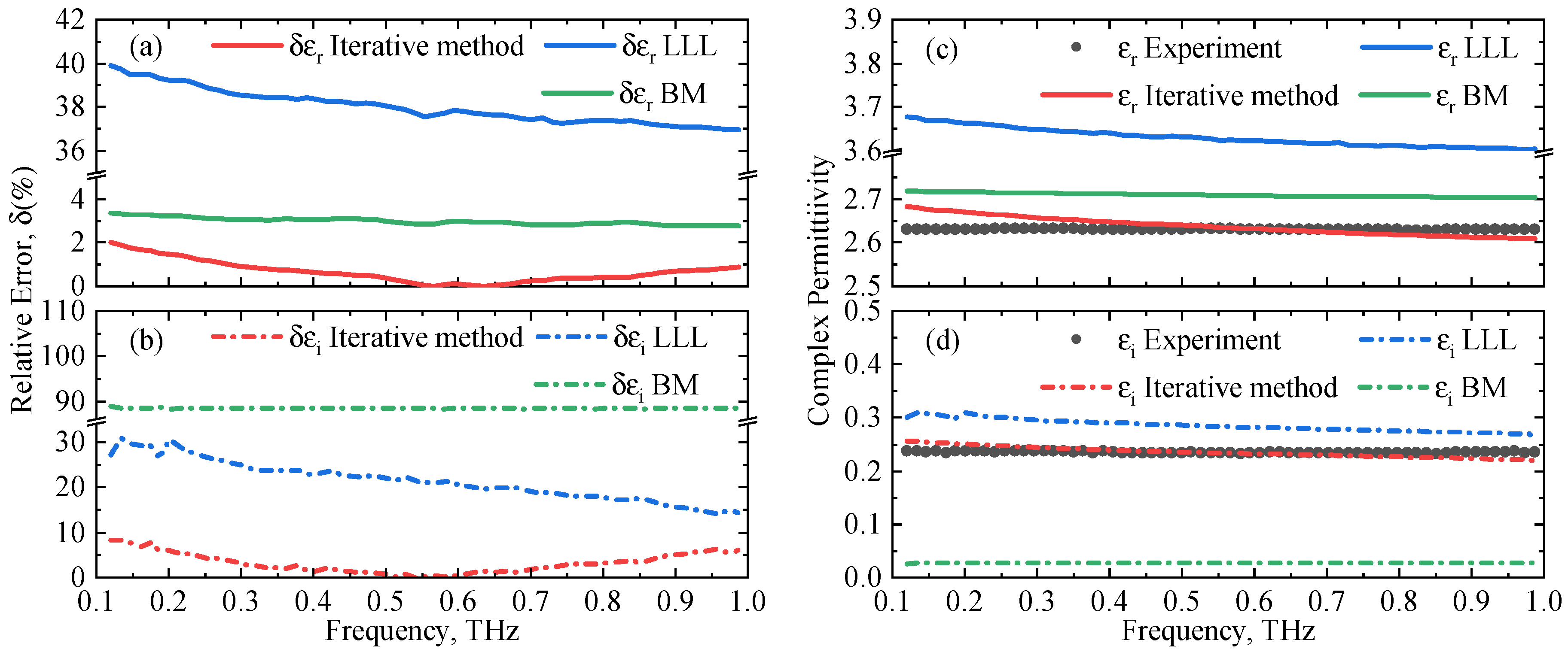
4.1. Titannium Dioxide, Silver and Low Density Polyethylene
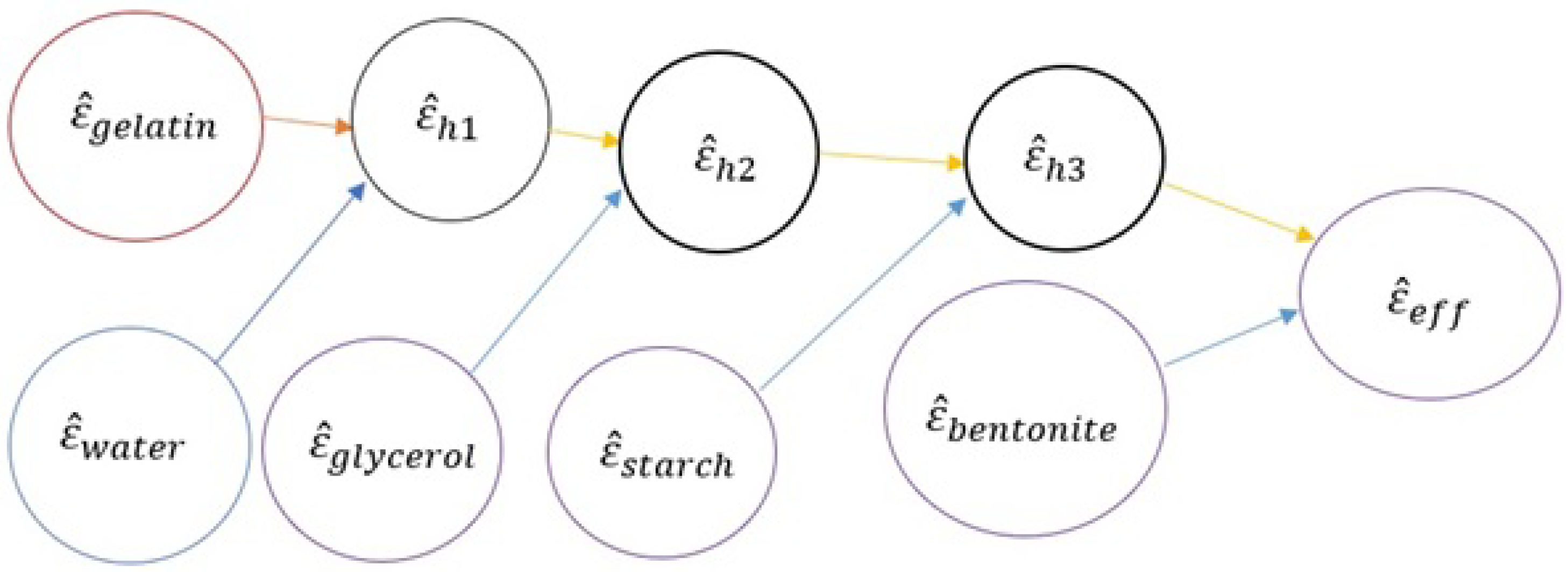
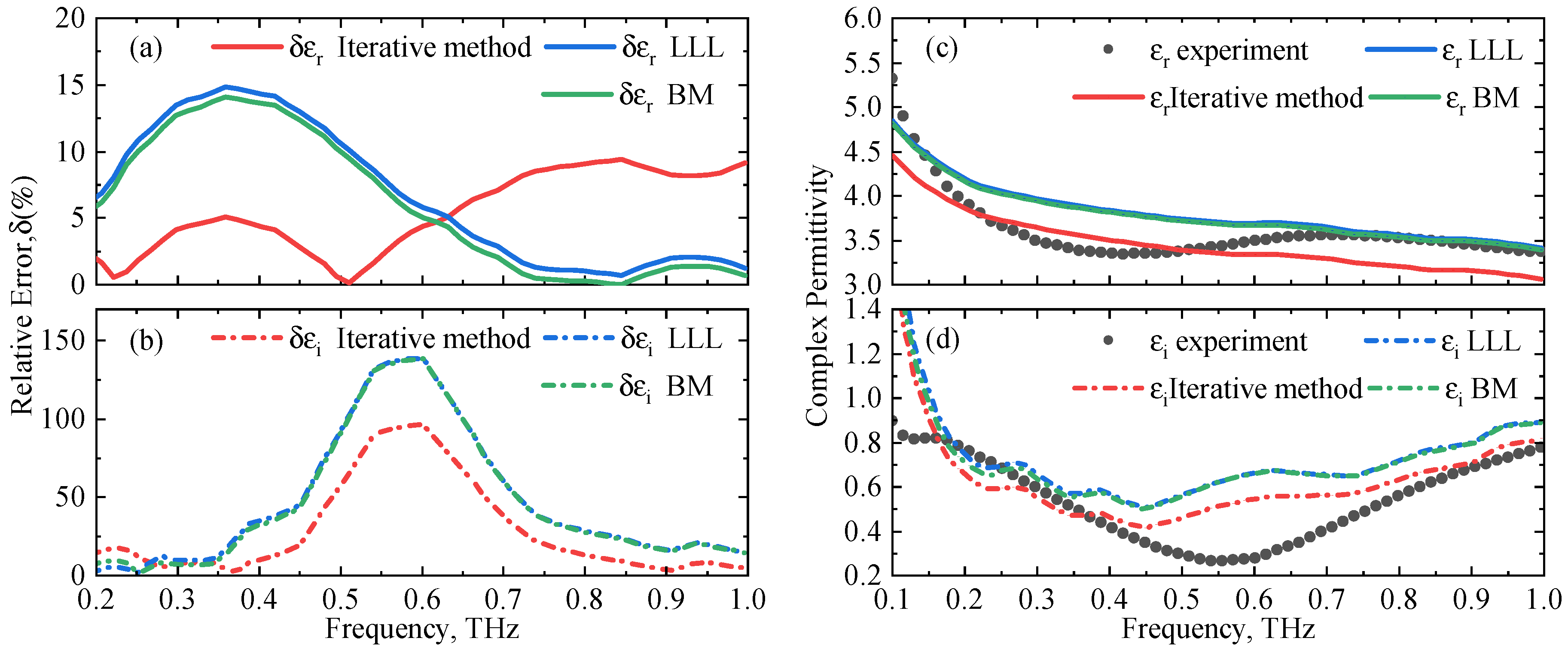
4.2. Gelatin, Water, Glycerin, Starch, Bentonite
4.3. Gelatin, Water and Oil
5. Conclusions
Author Contributions
Funding
Conflicts of Interest
Abbreviations
| THz | Terahertz |
| TDS | Time-domain spectroscopy |
| EMT | Effective medium theory |
| BM | Bruggeman |
| LLL | Landau-Lifshitz-Looyenga |
References
- Fischer, B.; Walther, M.; Jepsen, P.U. Far-infrared vibrational modes of DNA components studied by terahertz time-domain spectroscopy. Phys. Med. Biol. 2002, 47, 3807. [Google Scholar] [CrossRef]
- Cheon, H.; Yang, H.j.; Lee, S.H.; Kim, Y.A.; Son, J.H. Terahertz molecular resonance of cancer DNA. Sci. Rep. 2016, 6, 37103. [Google Scholar] [CrossRef] [PubMed]
- Markelz, A.; Roitberg, A.; Heilweil, E.J. Pulsed terahertz spectroscopy of DNA, bovine serum albumin and collagen between 0.1 and 2.0 THz. Chem. Phys. Lett. 2000, 320, 42–48. [Google Scholar] [CrossRef]
- Xie, L.; Yao, Y.; Ying, Y. The application of terahertz spectroscopy to protein detection: A review. Appl. Spectrosc. Rev. 2014, 49, 448–461. [Google Scholar] [CrossRef]
- Grognot, M.; Gallot, G. Quantitative measurement of permeabilization of living cells by terahertz attenuated total reflection. Appl. Phys. Lett. 2015, 107, 103702. [Google Scholar] [CrossRef]
- Zou, Y.; Li, J.; Cui, Y.; Tang, P.; Du, L.; Chen, T.; Meng, K.; Liu, Q.; Feng, H.; Zhao, J.; et al. Terahertz spectroscopic diagnosis of myelin deficit brain in mice and rhesus monkey with chemometric techniques. Sci. Rep. 2017, 7, 1–9. [Google Scholar] [CrossRef]
- Woodward, R.; Wallace, V.; Arnone, D.; Linfield, E.; Pepper, M. Terahertz pulsed imaging of skin cancer in the time and frequency domain. J. Biol. Phys. 2003, 29, 257–259. [Google Scholar] [CrossRef]
- Ashworth, P.C.; Pickwell-MacPherson, E.; Provenzano, E.; Pinder, S.E.; Purushotham, A.D.; Pepper, M.; Wallace, V.P. Terahertz pulsed spectroscopy of freshly excised human breast cancer. Opt. Express 2009, 17, 12444–12454. [Google Scholar] [CrossRef]
- Wahaia, F.; Kasalynas, I.; Seliuta, D.; Molis, G.; Urbanowicz, A.; Silva, C.D.C.; Carneiro, F.; Valusis, G.; Granja, P.L. Study of paraffin-embedded colon cancer tissue using terahertz spectroscopy. J. Mol. Struct. 2015, 1079, 448–453. [Google Scholar] [CrossRef]
- Wahaia, F.; Kasalynas, I.; Seliuta, D.; Molis, G.; Urbanowicz, A.; Silva, C.D.C.; Carneiro, F.; Valusis, G.; Granja, P.L. Terahertz spectroscopy for the study of paraffin-embedded gastric cancer samples. J. Mol. Struct. 2015, 1079, 391–395. [Google Scholar] [CrossRef]
- Tuncer, E.; Gubański, S.M.; Nettelblad, B. Dielectric relaxation in dielectric mixtures: Application of the finite element method and its comparison with dielectric mixture formulas. J. Appl. Phys. 2001, 89, 8092–8100. [Google Scholar] [CrossRef]
- Markel, V.A. Introduction to the Maxwell Garnett approximation: Tutorial. JOSA A 2016, 33, 1244–1256. [Google Scholar] [CrossRef] [PubMed]
- Dube, D. Study of Landau-Lifshitz-Looyenga’s formula for dielectric correlation between powder and bulk. J. Phys. D Appl. Phys. 1970, 3, 1648. [Google Scholar] [CrossRef]
- Landau, L.D.; Lifshitz, E.M.; Pitaevskii, L.P.; Sykes, J.B.; Bell, J.S.; Kearsley, M.J. Electrodynamics of Continuous Media; Elsevier: Amsterdam, The Netherlands, 2013; Volume 8. [Google Scholar]
- Looyenga, H. Dielectric constants of heterogeneous mixtures. Physica 1965, 31, 401–406. [Google Scholar] [CrossRef]
- Nelson, S.; You, T.S. Relationships between microwave permittivities of solid and pulverised plastics. J. Phys. D Appl. Phys. 1990, 23, 346. [Google Scholar] [CrossRef]
- Rutz, F.; Koch, M.; Khare, S.; Moneke, M. Quality control of polymeric compounds using terahertz imaging. In Terahertz and Gigahertz Electronics and Photonics IV; 2005; Volume 5727, pp. 115–122. [Google Scholar]
- Chen, W.; Kirihara, S.; Miyamoto, Y. Fabrication of three-dimensional micro photonic crystals of resin-incorporating TiO2 particles and their terahertz wave properties. J. Am. Ceram. Soc. 2007, 90, 92–96. [Google Scholar] [CrossRef]
- Azad, A.K.; Zhao, Y.; Zhang, W.; He, M. Effect of dielectric properties of metals on terahertz transmission in subwavelength hole arrays. Opt. Lett. 2006, 31, 2637–2639. [Google Scholar] [CrossRef]
- D’Angelo, F.; Mics, Z.; Bonn, M.; Turchinovich, D. Ultra-broadband THz time-domain spectroscopy of common polymers using THz air photonics. Opt. Express 2014, 22, 12475–12485. [Google Scholar] [CrossRef]
- Zhang, T.; Zakharova, M.; Vozianova, A.; Podshivalov, A.; Fokina, M.; Nazarov, R.; Kuzikova, A.; Demchenko, P.; Uspenskaya, M.; Khodzitsky, M. Terahertz optical and mechanical properties of the gelatin-starch-glycerol-bentonite biopolymers. J. Biomed. Photonics Eng. 2020, 6, 020304. [Google Scholar] [CrossRef]
- Truong, B.C.; Fitzgerald, A.J.; Fan, S.; Wallace, V.P. Concentration analysis of breast tissue phantoms with terahertz spectroscopy. Biomed. Opt. Express 2018, 9, 1334–1349. [Google Scholar] [CrossRef]
- Yang, X.; Zhao, X.; Yang, K.; Liu, Y.; Liu, Y.; Fu, W.; Luo, Y. Biomedical applications of terahertz spectroscopy and imaging. Trends Biotechnol. 2016, 34, 810–824. [Google Scholar] [CrossRef] [PubMed]
- Fan, S.; Ung, B.; Parrott, E.P.; Pickwell-MacPherson, E. Gelatin embedding: A novel way to preserve biological samples for terahertz imaging and spectroscopy. Phys. Med. Biol. 2015, 60, 2703. [Google Scholar] [CrossRef] [PubMed]


Publisher’s Note: MDPI stays neutral with regard to jurisdictional claims in published maps and institutional affiliations. |
© 2020 by the authors. Licensee MDPI, Basel, Switzerland. This article is an open access article distributed under the terms and conditions of the Creative Commons Attribution (CC BY) license (http://creativecommons.org/licenses/by/4.0/).
Share and Cite
Nazarov, R.; Zhang, T.; Khodzitsky, M. Effective Medium Theory for Multi-Component Materials Based on Iterative Method. Photonics 2020, 7, 113. https://doi.org/10.3390/photonics7040113
Nazarov R, Zhang T, Khodzitsky M. Effective Medium Theory for Multi-Component Materials Based on Iterative Method. Photonics. 2020; 7(4):113. https://doi.org/10.3390/photonics7040113
Chicago/Turabian StyleNazarov, Ravshanjon, Tianmiao Zhang, and Mikhail Khodzitsky. 2020. "Effective Medium Theory for Multi-Component Materials Based on Iterative Method" Photonics 7, no. 4: 113. https://doi.org/10.3390/photonics7040113
APA StyleNazarov, R., Zhang, T., & Khodzitsky, M. (2020). Effective Medium Theory for Multi-Component Materials Based on Iterative Method. Photonics, 7(4), 113. https://doi.org/10.3390/photonics7040113