Article

Monitoring of OSNR Using an Improved Binary Particle Swarm Optimization and Deep Neural Network in Coherent Optical Systems

1
College of Intelligent Science and Technology, National University of Defense Technology, Changsha 410073, China
2
College of Electric and Information Engineering, Hunan University of Technology, Changsha 412007, China
*
Author to whom correspondence should be addressed.
Photonics 2019, 6(4), 111; https://doi.org/10.3390/photonics6040111
Submission received: 30 August 2019 / Revised: 16 October 2019 / Accepted: 23 October 2019 / Published: 25 October 2019

Abstract

:
A novel technique is proposed to implement optical signal-to-noise ratio (OSNR) estimation by using an improved binary particle swarm optimization (IBPSO) and deep neural network (DNN) based on amplitude histograms (AHs) of signals obtained after constant modulus algorithm (CMA) equalization in an optical coherent system. For existing OSNR estimation models of DNN and AHs, sparse AHs with valid features of original data are selected by IBPSO algorithm to replace the original, and the sparse sets are used as input vector to train and test the particle swarm optimization (PSO) optimized DNN (PSO-DNN) network structure. Numerical simulations have been carried out in the OSNR ranges from 10 dB to 30 dB for 112 Gbps PM-RZ-QPSK and 112 Gbps PM-NRZ-16QAM signals, and results show that the proposed algorithm achieves a high OSNR estimation accuracy with the maximum estimation error is less than 0.5 dB. In addition, the simulation results with different data input into the deep neural network structure show that the mean OSNR estimation error is 0.29 dB and 0.39 dB under original data and 0.29 dB and 0.37 dB under sparse data for the two signals, respectively. In the future dynamic optical network, it is of more practical significance to reconstruct the original signal and analyze the data using sparse observation information in the face of multiple impairment and serious interference. The proposed technique has the potential to be applied for optical performance monitoring (OPM) and is helpful for better management of optical networks.

1. Introduction

With the application of high-speed and large-capacity optical communication technologies such as reconfigurable optical add-drop multiplexer (ROADM), dense wavelength division multiplexing (DWDM), polarization multiplexing, and coherent optical communication to optical communication systems, the capacity and rate of optical networks are changing at a constantly changing speed. In the future, the optical network will continue to develop towards the goal of being more flexible, high-speed and dynamic, however, with the increasing complexity of network structure and the aggravation of signal impairment, the reliability of optical fiber communication system and optical network will be reduced.
It is predicted that the future optical communication system will no longer be a relatively static network system that operates completely following established norms. The dynamic link structure will change with the temperature, component replacement, aging and optical fiber maintenance, and the optical nodes that can achieve “Plug and Play” will be required to better allocate optical network resources. This phenomenon improves the transparency of an optical system but increases the complexity of network management [1]. The capacity of optical networks has been growing steadily, and the network architectures are becoming more dynamic, complex, and transparent. Optical signals in high-speed optical fiber networks are vulnerable to various transmission impairments, which can change dynamically with time. Therefore, an appropriate monitoring mechanism must be established throughout the optical network to provide accurate and real-time information on the quality of transmission links and the health of optical signals. optical performance monitoring (OPM) technology detects the performance parameters of transmission links or optical network nodes in optical networks, and understands the network status and signal transmission status in real time, and therefore processes and ensures the normal network operation and signal transmission. It is of great significance to guarantee the performance of signal transmission and optimize the allocation and management of network resources. Therefore, in order to realize the next generation dynamic reconfigurable optical network, it is necessary to monitor the important parameters, isolate faults in time, and optimize the processing to ensure the transmission quality of the network [2,3].
The optical signal-to-noise ratio (OSNR) is one of the key parameters of OPM. It can realize fault management of an optical transmission system and network, including fault diagnosis and location [4]. It can be used to estimate the bit error rate (BER) and signal quality of the system, and it can directly indicate the channel quality and may realize the management, configuration, and optimization of dynamic reconfigurable optical networks. OSNR can intuitively reflect the change of signal power and noise power of the transmitted optical signal, and it is related to the BER at the end of the optical signal transmitted through the optical amplification link. OSNR is transparent to the bit rate and modulation format of optical signals and suitable for dynamic reconfigurable optical networks. Therefore, OSNR has become an important indicator of optical path performance in OPM and can be used to directly reflect signal quality and system performance. Moreover, understanding OSNR can help effectively utilize available network resources. OSNR is a direct indication of link transmission performance in all kinds of impairment to be monitored, regardless of modulation format. Therefore, the monitoring of OSNR is essential for the overall effective operation of network management system (NMS) and network [5].
At present, most of the practical application of OSNR monitoring methods are out-of-band OSNR testing methods, including the monitoring method based on tunable optical filter [6], arrayed waveguide grating [7], and so on. However, this kind of test method apparently has not met the requirements of the next generation of intelligent optical networks, which changes from traditional out-of-band OSNR monitoring to in-band OSNR monitoring with higher monitoring accuracy. With the rapid development of high-speed coherent optical communication systems, some in-band OSNR monitoring technologies for coherent optical communication systems have been proposed, including Stokes parameters [8], delay-line interferometer (DLI) [9], four-wave mixing (FWM) [10], statistical moments [11], normalized autocorrelation function [12], error vector magnitude (EVM) [13], asynchronous delay sampling [14], and Golay sequence [15] based methods. However, many of the OSNR monitoring technologies mentioned above require additional hardware and monitoring equipment, which increases the complexity and cost of the system. Some technologies perform well under weak input power and weak nonlinearity systems and have high requirements for linear impairment compensation of receiving channel. In addition, some techniques based on training sequence may reduce the spectral efficiency of the system and need to be applied to the optical fiber nonlinear scene in the state of high transmission power. In view of this, the various OSNR monitoring technologies mentioned above have been unable to meet the continuous development of optical communication systems toward high-speed and high-frequency spectrum utilization. Therefore, in modern optical communication system, with the change of signal rate, transmission mode, and networking mode, the development of OSNR monitoring technology is also developing in the direction of high-speed, intelligent, digital and low-cost systems.
In recent years, deep learning (DL) is the mainstream research direction of machine learning. It is also a part of the framework of artificial intelligence (AI) [16]. Its essence is to build a multilayer computing model and learn the manifestation of data through multilayer abstraction. This technology has made technological breakthroughs in most research fields, including data mining [17], visual target detection [18], speech recognition [19], target recognition [20], quality of transmission (QoT) prediction [21], and medical diagnostic [22], as well as greatly improved the learning performance of related systems. Compared with traditional machine learning, DL is constantly deepened on the basis of artificial neural network theory. By adopting universal learning process and layer-by-layer learning feature representation, the impact of the introduction of artificial features on the system is weakened. At present, DL technology has also been well used in optical communications to promote the development of intelligent systems [23]. The methods of OPM using machine learning include support vector machine (SVM) [24], artificial neural network (ANN) [25], generalized regression neural network (GRNN) [26], and convolutional neural network (CNN) [27]. Recently, the use of deep neural network (DNN) instead of shallow ANN for optical performance monitoring has been extensively studied. DNN is a network structure with multiple hidden layers between the input and output layers. The additional layers of DNN will automatically extract input features, so that complex data can be modeled by fewer units than shallow networks [28].
In this paper, we demonstrate a technique which employs the improved binary particle swarm optimization (IBPSO) algorithm and the particle swarm optimization optimized deep neural network (PSO-DNN) structure in optical coherent receivers for OSNR monitoring. Particle swarm optimization (PSO) is a kind of swarm intelligence optimization algorithm in the field of computational intelligence. It is a global optimization intelligent algorithm that uses the foraging behavior characteristics of biological populations to simulate and solve practical optimization problems [29]. PSO is a meta-heuristic as it makes few or no assumptions about the problem being optimized and can search very large spaces of candidate solutions [30,31]. Compared with the other evolutionary algorithm such as artificial fish swarm algorithm [32], genetic algorithm [33,34], artificial bee colony algorithm [35,36], and simulated annealing algorithm [37], the most important advantages of PSO are the few parameters needed to adjust and the easy implementation. IBPSO follows the action of chromosomes in genetic algorithm (GA) and sparsely calculates the eigenvectors of the input AHs. In many practical problems, sparse signals can provide enough information, such as head image recognition [38], sound location [39], and target tracking [40]. In the proposed scheme, first the equivalent AHs sparse dataset is obtained by the IBPSO as the eigenvector input of the DNNs, and then the optimization training is conducted on two DNN modules for 112 Gbps PM-RZ-QPSK and 112 Gbps PM-NRZ-16QAM signals, respectively, through PSO to obtain the accurate estimation of OSNR. Experimental results obtained show that the proposed method can achieve a higher precision estimation of OSNR than the existing methods. In addition, this technology does not require additional monitoring equipment or any modifications to the transmitter. As the dimension of the input signal set AHs decreases, the corresponding neural network structure is simplified correspondingly, and the estimation accuracy is still relatively high.
The rest of this paper is structured as follows. Section 2 introduces the OSNR monitoring based on the conventional DNN and the improved binary particle swarm optimization and deep neural network (IBPSO-DNN) method trained with AHs in detail. Section 3 describes the structure of the OSNR monitoring experimental configuration of PM-RZ-QPSK and PM-NRZ-16QAM signals. Some simulation results and discussion are presented in Section 4. Finally, Section 5 sums up the conclusions.

2. Principles of the Proposed Method

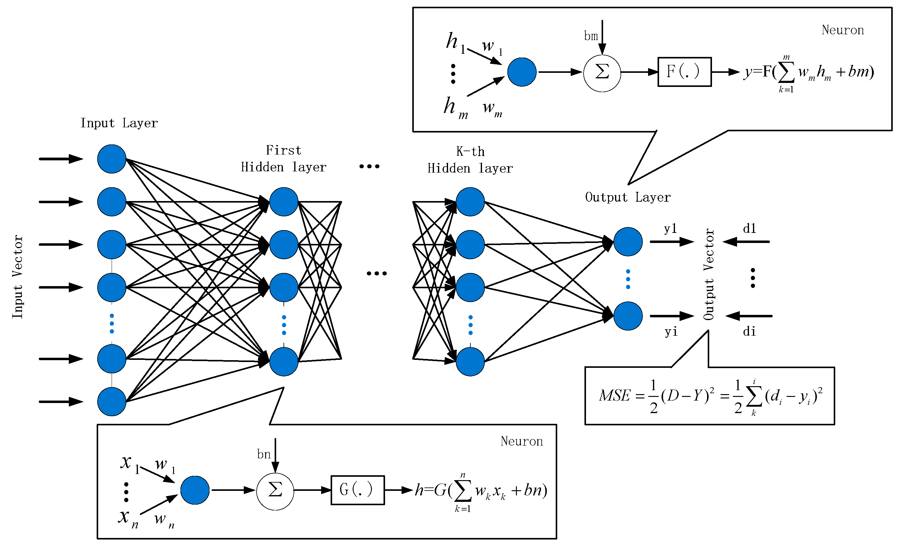
2.1. OSNR Monitoring Based on the Conventional DNN Trained with AHs

Consider a coherent optical transmission system, its coherent receiver and digital signal processing (DSP) architecture, including the proposed OSNR monitoring stage, as shown in Figure 1. The received signal in the digital coherent receiver adopts the standard signal processing algorithms in the DSP unit, including normalization, resampling and phase-orthogonal (IQ) imbalance compensation, and then followed by chromatic dispersion (CD) compensation and timing phase recovery algorithm independent of the standard modulation format. Next, we use equalization based on CMA to solve polarization demultiplexing and compensate almost all linear transmission impairments [41]. As can be seen from Figure 1, the data for OSNR monitoring is the output signal after CMA equalization. After this stage, the signal is mainly affected by the amplified spontaneous emission (ASE) noise.
Figure 2 and Figure 3 show the constellation diagram and the corresponding amplitude histograms of PM-RZ-QPSK and PM-NRZ-16QAM signals after CMA equalization, as well as the constellation diagram after carrier phase estimation. AHs are generated by data samples obtained after CMA equalization module with 100 bins. We choose OSNR monitoring after CMA equalization instead of carrier phase estimation because the former only needs a few DSP units, which reduces the complexity of OPM devices, while the latter needs to process additional AHs, which increases the computational complexity and time. It can be clearly seen from the two figures that their corresponding AHs show unique and distinct signatures for different OSNRs and modulation formats. Therefore, the sensitivity of AHs to OSNR can be used as an estimated feature of OSNR monitoring. Then, the pattern recognition technology based on conventional DNN is used to estimate OSNR by using the relevant features of AHs.
After obtaining the characteristic data for estimating OSNR, it was input into DNN structure as input data for training and test. The schematic diagram of the fully connected conventional DNN (no optimization algorithm) is shown in Figure 4. It includes an input layer, multiple hidden layers, and an output layer. The mean square error (MSE) formula of the output end, the output of the hidden layer, and the output layer neuron are shown in Figure 4. Where, x is the input vector, d is the predicted value of output, w and b are the weights and biases in the DNN structure, and G ( . ) and F ( . ) are the activation functions of the hidden layer and the output layer including Tanh, Sigmoid, ReLU and Linear, Sigmoid, and Softmax, respectively. The weights and biases of DNN are initialized randomly, and the whole network is trained by an iterative algorithm. The training can be stopped by adjusting the parameters according to the MSE between the current output and the label, until the error converges or reaches a certain iteration set value. In the conventional OSNR estimation algorithm, the input vector is composed of 100 × 1 bin counts in the AHs dataset, which is input into different DNN structures of two signals. Considering the estimated value of OSNR, the output layer neuron is 1 and the output value is scalar.

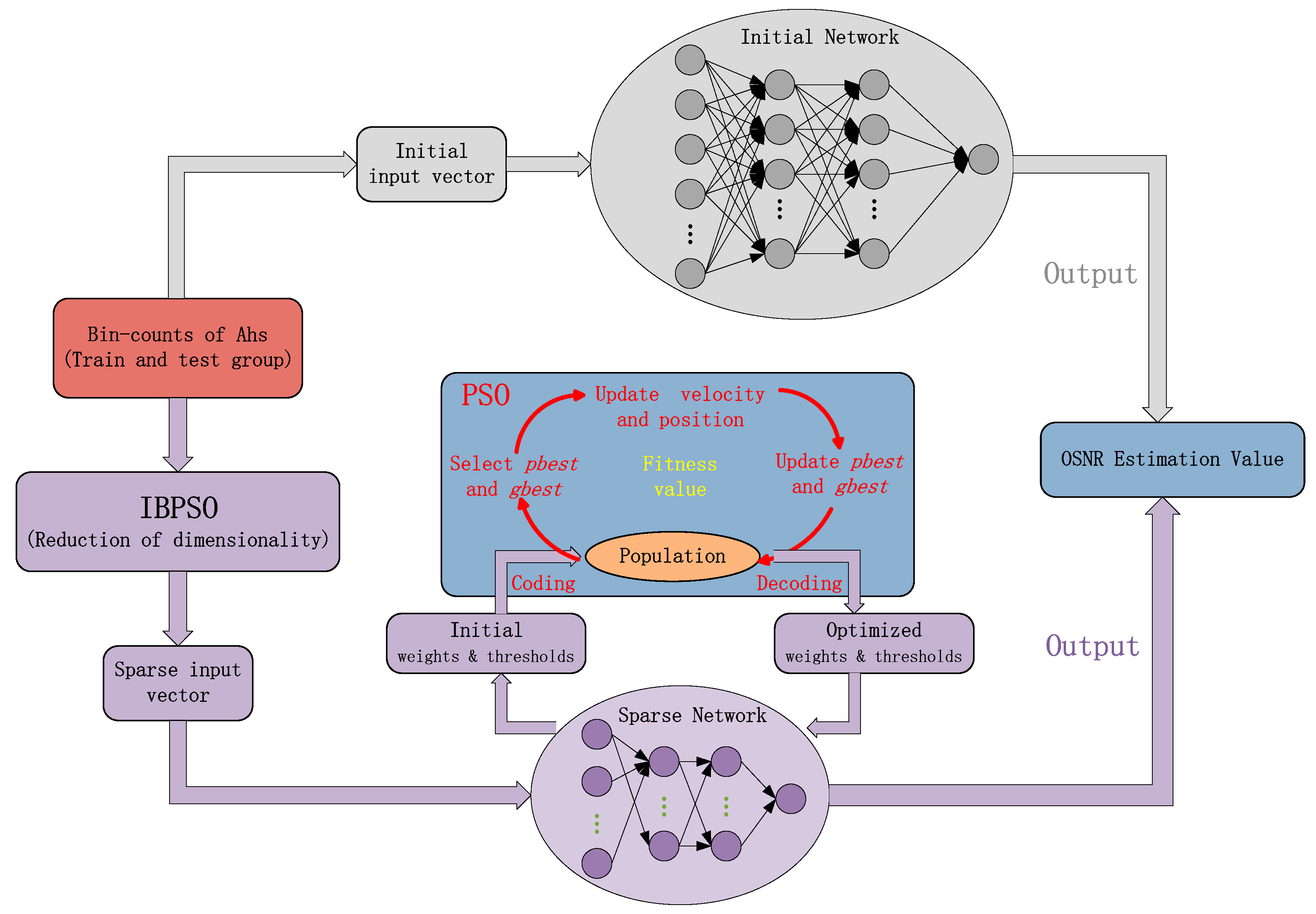
2.2. OSNR Monitoring Based on the IBPSO-Based DNN Trained with AHs

With the development of evolutionary computation, people gradually combine intelligent optimization algorithm with neural network, and use various optimization methods to train neural network. Because the intelligent optimization algorithm has strong global convergence ability and robustness, it does not need the feature information. Therefore, the combination of the two gives play to the generalization mapping ability of the neural network, and also improves the convergence speed and learning ability of the neural network. Common intelligent optimization algorithms include GA [42], ant colony optimization (ACO) algorithm [43], and PSO. Among them, GA cannot converge effectively in a limited time and ACO needs a long search time and is prone to premature convergence because of its lack of initial information and slow solution speed. As a swarm intelligence optimization algorithm, PSO employs the cooperative mechanism of swarm solutions to produce the optimal solution iteratively. In addition, the concept of PSO is simple and easy to implement, and there are few parameters to be adjusted.

2.2.1. Principle of Particle Swarm Optimization (PSO)

The basic idea of PSO is that the potential solution of each optimization problem is a particle in the search space. All particles have a fitness value determined by the function of optimization. Each particle has a velocity vector to determine the direction and distance of their movement, and then the particles follow the search of the current optimal particle in the solution space. The PSO algorithm is initialized as a group of random particles, and then the optimal solution is found by iteration. The particle updates itself by tracking two extremes values in each iteration. The first extreme value is the best solution found by the particle itself until the current moment, which is called individual best value. The other is the best solution found by the whole population until the current moment, which is called the global best value.
Suppose that in a D-dimensional target search space, there are n particles forming a population X = ( X 1 , X 2 , , X n ) , where the ith particle is expressed as a D-dimensional vector x i = ( x i 1 , x i 2 , , x i D ) , representing the position in the D-dimensional search space of the ith particle, and also representing a potential solution of the problem. According to the objective function, the fitness value corresponding to each particle position x i can be calculated. The velocity of the ith particle is v i = ( v i 1 , v i 2 , , v i D ) , its previous best position in the history of each particle is p i = ( p i 1 , p i 2 , , p i D ) , and the best position associated with the best particle in the population is p g = ( v g 1 , v g 2 , , v g D ) . During the evolutionary process, the best previous position of a particle is recorded as the personal best p b e s t and the best position obtained by the population thus far is called g b e s t .
In each iteration, the particle updates its velocity and position through individual and global extremum. The updating formula is as follows:
v i d ( t + 1 ) = ω v i d ( t ) + c 1 r a n d ( ) ( p i d x i d ( t ) ) + c 2 r a n d ( ) ( p g d x i d ( t ) )
x i d ( t + 1 ) = x i d ( t ) + v i d ( t + 1 )
where, ω is inertia weight, i = 1 , 2 , , n , d = 1 , 2 , , D , t is the current iteration number. The learning factor c 1 and c 2 are non-negative constants. These two constants enable the particles to self-summarize and learn from the excellent individuals in the group, thus, approaching their own historical optimum and the global optimum within the group or in the field. r a n d ( ) is a random function evaluated in the range [0,1]. The first part expresses the influence of historical inertia on the present, the second part shows the recognition and reflection of particles on themselves, and the third part expresses the learning, comparison, and imitation of particles on the whole population. v i d [ v max , v max ] is the current velocity of the ith particle, and v max is a non-negative number, that is, after the implementation of the velocity update formula, there are:
i f   v i d < v max ,   t h e n   v i d = v max i f   v i d > v max ,   t h e n   v i d = v max

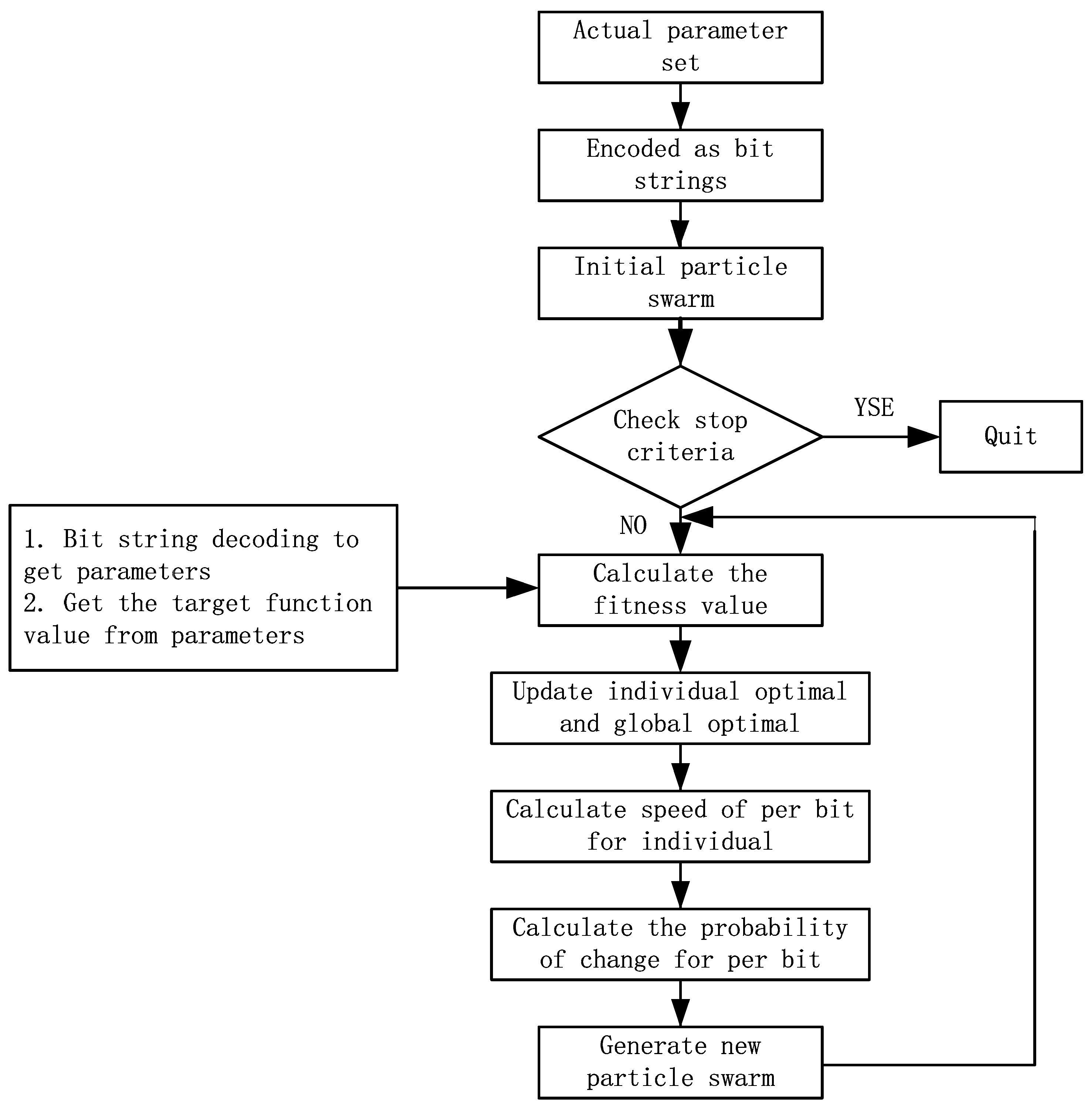
2.2.2. Principle of the IBPSO

Considering that the large input dataset in the DNN usage scenario will affect the convergence rate and computational complexity of DNN, therefore, it is necessary to conduct dimensionality reduction preprocessing for the data [44]. The common dimension reduction methods are principal component analysis (PCA) and partial least square (PLS). The disadvantage of PCA is that it is opposite to the original input variable, and the derived dimension may have no intuitive explanation. In addition, the implementation process of PLS is based on nonlinear iteration, which usually requires hypothesis or transformation of the original sample data, which is difficult to satisfy in practical problems. Therefore, the IBPSO algorithm was introduced to get an equivalent sparse input vector set to represent the original data by referring to the principle of sparse sampling and the role of chromosomes in GA, which improved the effect of data execution and data dimension reduction, and it was less affected by the testing process.
The particles of a traditional binary particle swarm optimization (BPSO) algorithm are composed of binary strings [45]. In the specific dimension, the probability distribution with particle velocity as the main function generates the particle position randomly. Each binary bit utilizes Equation (1) to generate speed, and its velocity value is converted into the probability of transformation, that is, the chance of the bit variable to take a value of 1. In order to indicate that the velocity value is the probability of binary bit picking 1, the value of velocity is mapped to [0,1]. The mapping function is generally adopted as sigmoid function:
S ( v i d ) = S i g m o i d ( v i d ) = 1 1 + exp ( v i d )
where S denotes the probability that position x i d takes 1, and the particle changes its position by the following formula:
x i d = { 1 i f   r a n d ( ) S ( v i d ) 0 o t h e r w i s e
It should be noted that the value of sigmoid function does not represent the probability of a bit change, only the probability of one bit take a value of 1. When the velocity of the particle v i d approaches 0 it means that the position of the particle x i d is consistent, and the sigmoid function demonstrates an equal probability of 0 or 1 for x i d . If it converges to the global optimal particle, its velocity is 0. At this point, according to the properties of sigmoid function, the most chance of bit change is 0.5. And the search is random and directionless. Therefore, the traditional BPSO algorithm is a global random search algorithm, which runs with iteration and has strong randomness.
In order to make the particle tend, more and more, to the optimal particle, and the algorithm converges to the global optimal particle, we change the mapping function to the following formula:
S ( v i d ) = { 1 2 1 + exp ( v i d ) v i d 0 2 1 + exp ( v i d ) 1 v i d > 0
Then, the updating formula of particle position is changed to the following form:
x i d = { 0 i f   r a n d ( ) S ( v i d ) x i d o t h e r w i s e w h e n   v i d < 0
x i d = { 1 i f   r a n d ( ) S ( v i d ) x i d o t h e r w i s e w h e n   v i d > 0
The purpose of the new mapping function is that when the velocity tends to 0, the value of the probability mapping function is 0. Secondly, when the value of the probability function is set to 0 and 1 in the form of Equations (7) and (8), this form can ensure that the value of bit is unchanged when the velocity is 0. When the velocity is negative, the bit can only be changed to 0, and when the velocity is positive, the bit can be changed to 1. In this way, the particle swarm can easily approach the global optimal particle eventually and, when the velocity is 0, the probability of a change rate of the particle bit is increased near 0. This idea is in agreement with the essence of particle swarm optimization.
With improvements to BPSO, IBPSO finds the best binary vector where each bit is associated with a feature. If a bit of the vector is 1, the feature is selected. If the bit is 0, the feature cannot be selected. We hope to divide the whole feature and eliminate the irrelevant features by their importance. This helps us to reduce the computational overhead, dimension features of datasets, and improve the estimation accuracy. The flow chart of the IBPSO algorithm and the process of optimizing DNN with joint IBPSO and PSO are shown as Figure 5 and Figure 6. As can be seen from Figure 6, the “initial network” is the conventional DNN for comparison and the fully connected DNN based on IBPSO has a simpler structure due to the reduced dimension of bin counts of AHs, which reduces the hardware complexity of the sampling module.

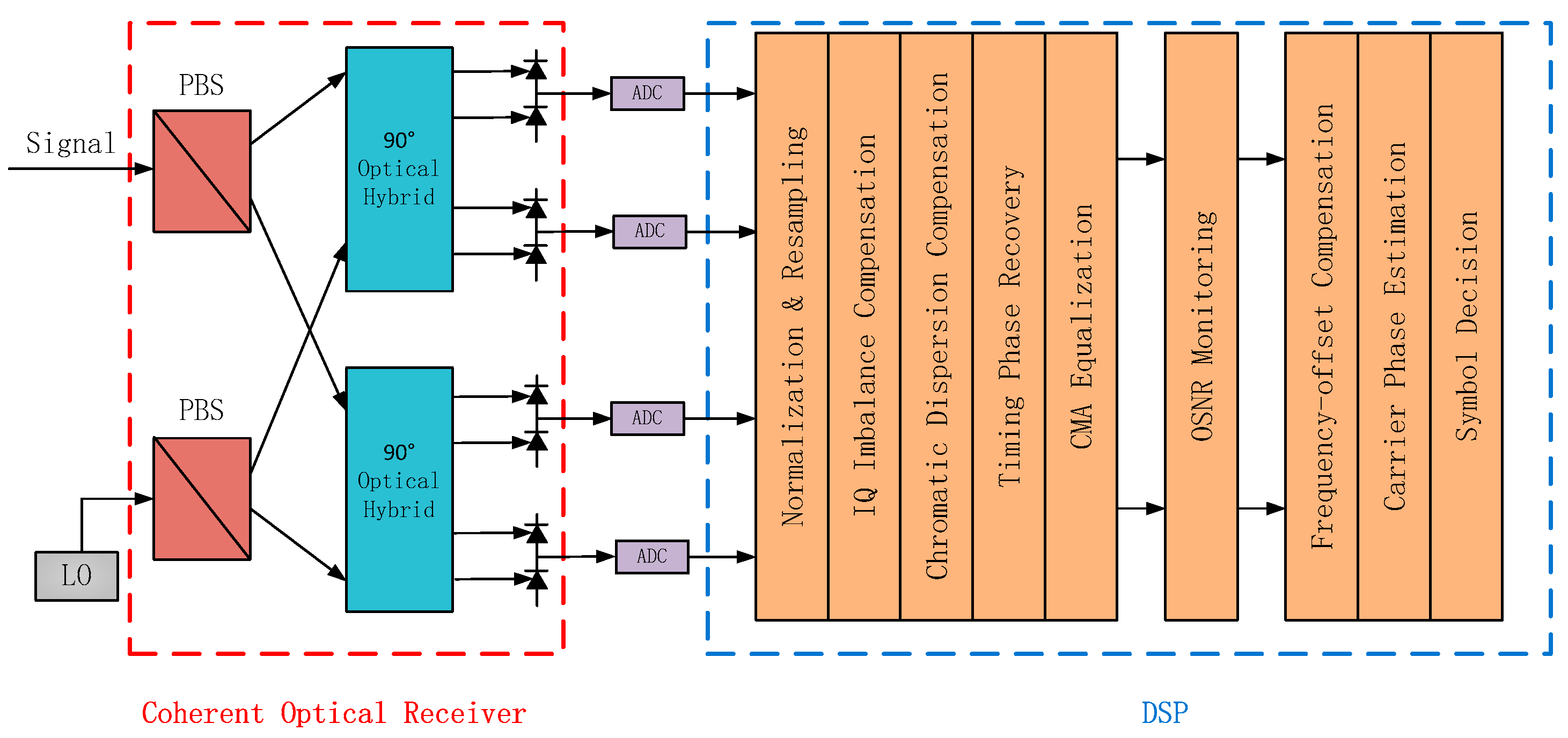
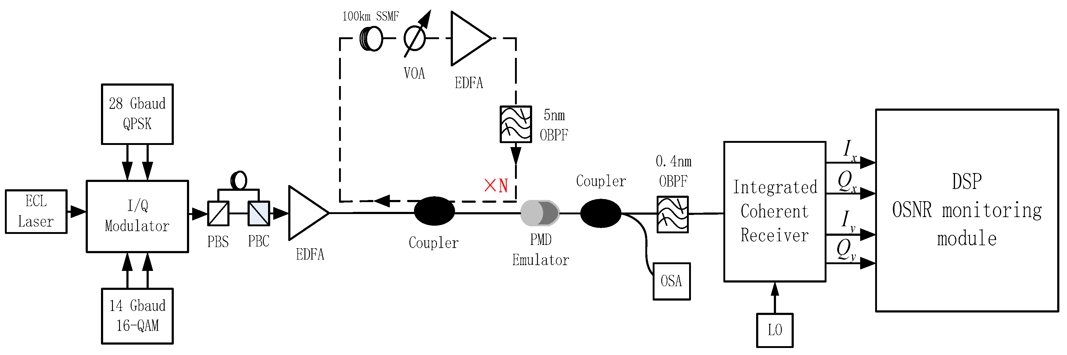
3. Experimental Setup

Experiments have been performed to demonstrate the validity of the proposed OSNR monitoring technique for 112 Gbps PM-RZ-QPSK and 112 Gbps PM-NRZ-16QAM systems. The experimental configuration is shown in Figure 7. At the transmitter, 28 Gbaud RZ-QPSK and 14 Gbaud NRZ-16QAM optical carrier signals are generated using an external cavity laser (ECL) and an I/Q modulator driven by multilevel electrical signals. ECL has a central wavelength of 1550 nm and its line width is 150 kHz. A polarization beam splitter (PBS) divides continuous laser generated by continuous wave laser into two groups of vertically polarized optical carriers. The data of pseudo-random binary sequence (PRBS) generator are transformed into corresponding modulator driving signals by level generator and modulation driver, and then modulated to two vertically polarized optical signals by IQ modulator. Finally, these two groups of orthogonal polarized optical signals are synthesized by polarization beam combiner (PBC) to obtain polarization multiplexing optical signals. Then, the two signals are amplified by erbium-doped fiber amplifier (EDFA) and transmitted through the optical fiber recirculation loop. The loop consists of a span of 100 km standard single mode fiber (SSMF), EDFA, a variable optical attenuator (VOA) placed before the EDFA and a 5 nm bandwidth optical bandpass filter (OBPF) for channel power equalization. The gain of EDFA is 20 dB and the noise figure (NF) is 4 dB. Variable amounts of CD and differential group delay (DGD) are induced by the fiber and polarization mode dispersion (PMD) emulator, respectively. The OSNR is adjusted in the range of 10 and 30 dB in steps of 2 dB, the CD is introduced in the range between 0 and 3400 ps/nm in steps of 200 ps/nm, and the DGD is introduced in the range of 0 and 20 ps in steps of 2 ps. At the output end of the loop, the real value of OSNR is measured by optical spectrum analyzer (OSA). The output optical signal is filtered by 0.4 nm bandwidth OBPF, and then detected by a coherent receiver. The line width of the local oscillator (LO) is 100 kHz, and the frequency offset is 1 GHz. The coherent detected signal is sampled by a real-time oscilloscope with a 50G sampling rate, and then input to the DSP module for offline processing.
A total of 200,000 amplitude samples for the whole experiment are obtained through offline processing. These samples are treated with 100 bin numbers to obtain 200 sets of AHs data, and thus the complete dataset of AHs is obtained. The equivalent sparse dataset of AHs is screened from the original dataset by the IBPSO algorithm. The OSNR monitoring system based on DNN and PSO adopts original and sparse datasets for training, respectively. The training set and test set are randomly selected as 80% and 20% of the AHs data and 10-fold cross-validation is also applied to validate the accuracy of the model and the results are not biased by the random train and test split.

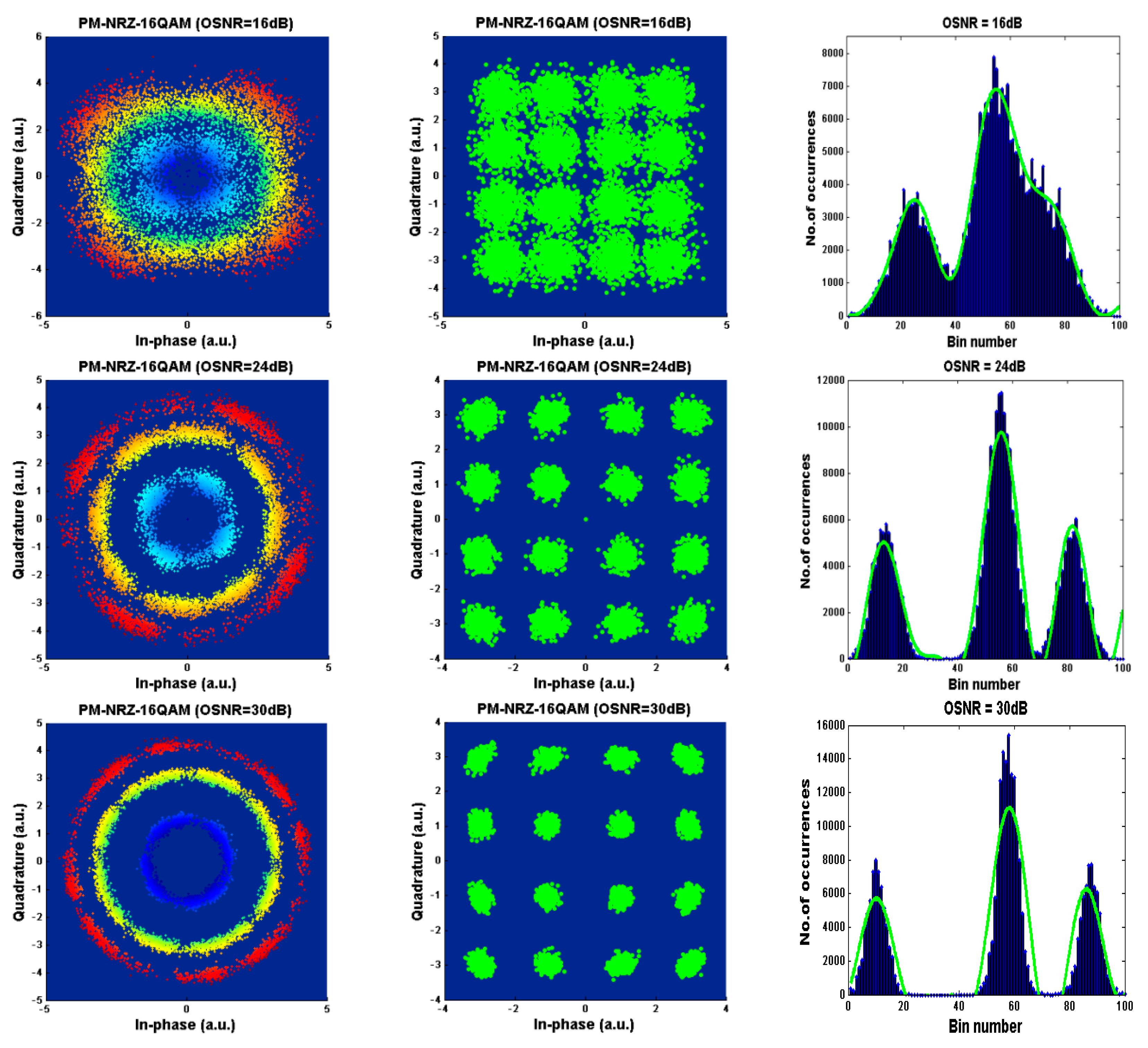
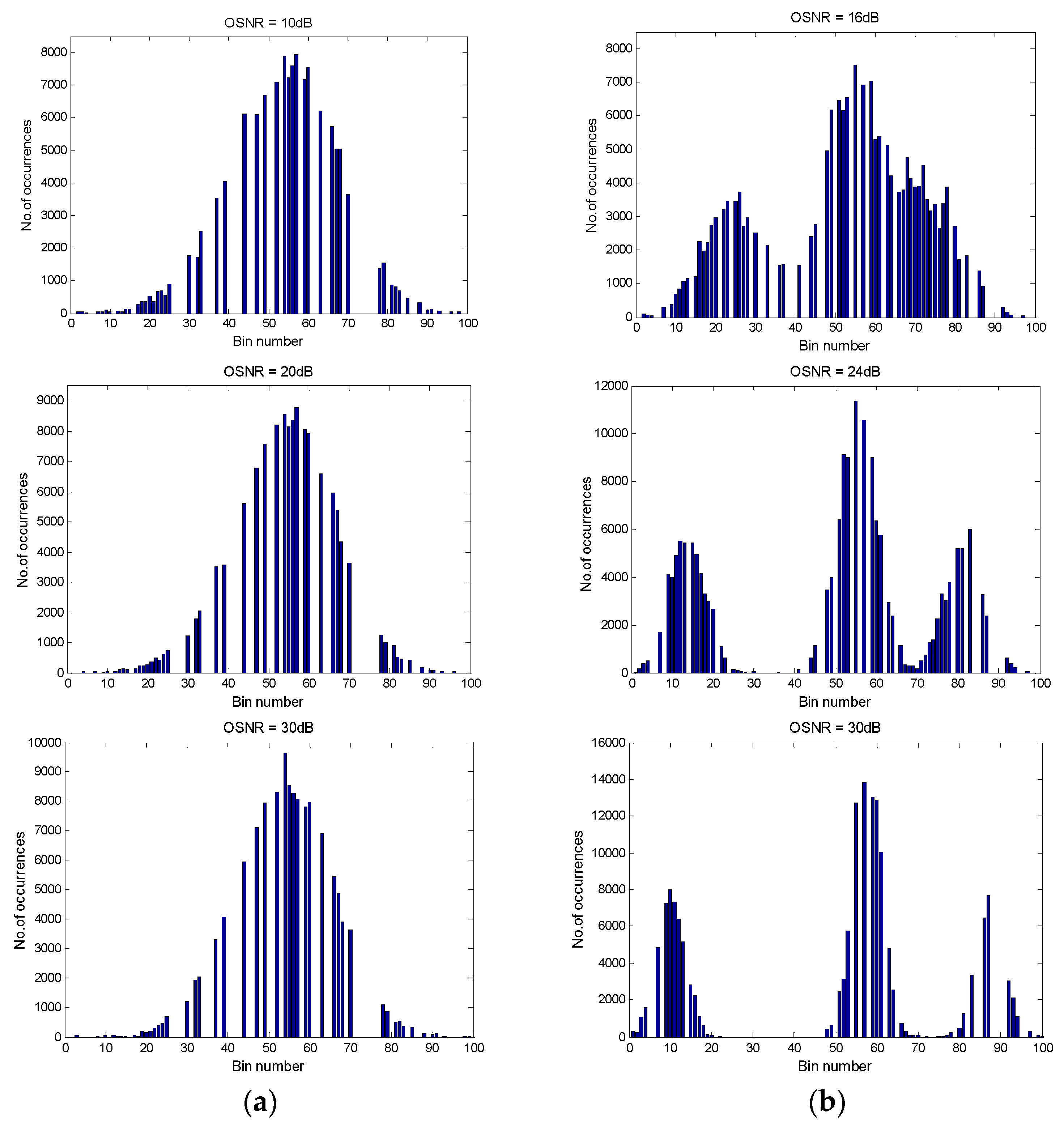
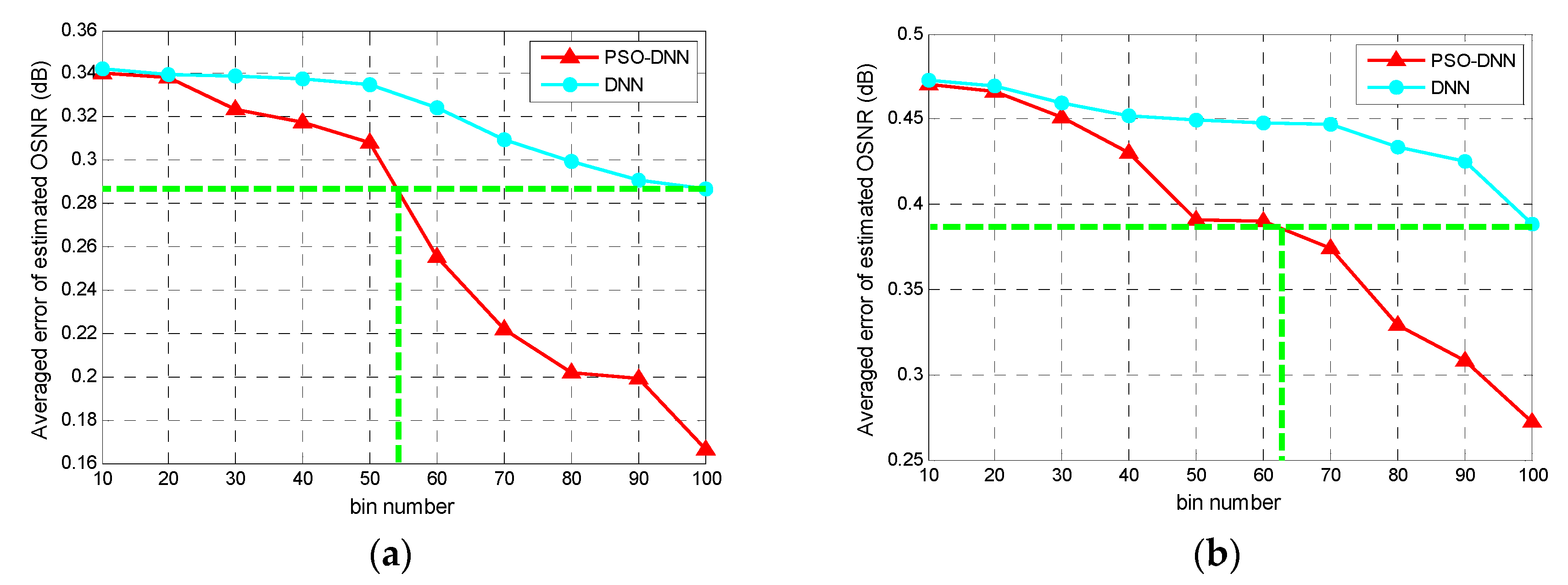
4. Results and Discussion

Considering that the larger dataset and more hidden layers have a greater impact on the neural network structure and iteration time of the neural network structure, this paper constructs a four-layer DNN structure which is illustrated in Figure 6. The number of input neuron nodes is equal to that of bin number, and the number of output neuron nodes is 1. The activation functions of the hidden layer and the output layer are Logsig and linear functions, respectively. We use the grid search method to optimize the number of hidden layer neuron nodes and get the optimal value of hidden layer neuron nodes when the fitness value reaches the minimum value. In order to find the relationship between bin number and OSNR estimation accuracy, we treat the total amplitude sample data according to AHs bin number of 10–100 (with step size of 10) to obtain different AHs bin counts. After the two signals are processed by DSP, each signal is transformed into a n i × 1 dimensional vector x = ( x 1 , x 2 , , x n i ) T , where n i = 10 , 20 , 30 , 40 , 50 , 60 , 70 , 80 , 90 , 100 is the AHs bin number and x = ( x 1 , x 2 , , x n i ) T is n i AHs bin counts. Therefore, this is the input data of PSO-DNN. Correspondingly, the input layer of PSO-DNN has n i neurons. For comparison, we input the same training set into the traditional DNN for training and test the conventional DNN and PSO-DNN with the same test set, respectively. Among them, the structures of neurons for PSO-DNN with 100 input nodes was trained and tested with complete AHs signal sets, 100-76-47-1 (input layer has 100 nodes, the two hidden layers have 76 and 47 nodes, and output layer has 1 node) and 100-79-62-1 for QPSK and 16QAM signals, respectively. The corresponding neuronal structures of conventional DNN are 100-77-52-1 and 100-62-53-1. In addition, the neuron structures of other bin numbers were obtained by grid search method, therefore, they are not listed one by one.
Through the simulations of PSO-DNN and conventional DNN by convergence training, the average estimation error of these two signals in OSNR of corresponding AHs bin number are calculated and mapped. The following simulation results are obtained by random selection as 80% and 20% of the AHs data for the training set and the test set and a 10-fold cross-validation is used to obtain the average results to ensure the model fits the training data well. As shown in the Figure 8, the average estimation error in OSNR of the two signals trends to decreases as the AHs bin number increases. For PM-RZ-QPSK and PM-NRZ-16QAM signals, the average error of PSO-DNN in OSNR is the same as that of conventional DNN when the bin number is about 53 and 62, that is, PSO-DNN can achieve the same OSNR estimation accuracy as conventional DNN with fewer neurons. It is worth noting that when the bin number is 100, PSO-DNN can achieve a smaller estimation error than conventional DNN, which indicates that PSO-DNN can achieve better estimation accuracy than conventional DNN when the number of neurons is the same. It can be seen that when the number of layers of the neural network structure is the same, the number of neurons in the input layer is the main factor of the complexity of the network structure and the modeling time. Therefore, compared with conventional DNN, PSO-DNN can achieve better estimation accuracy under the same complexity of neural network structure.
In order to achieve high estimation accuracy with fewer neuron nodes in the input layer, an IBPSO algorithm is introduced into the system to obtain equivalent sparse input vectors. Through repeated iterations of the IBPSO algorithm, the sparse AHs signal sets Q P S K and 16 Q A M of the two signals are statistically obtained by:
Q P S K = { x 1 , x 2 , x 3 , x 4 , x 7 , x 8 , x 9 , x 10 , x 12 , x 13 , x 14 , x 15 , x 17 , x 18 , x 19 , x 20 , x 21 , x 22 , x 23 , x 24 , x 25 , x 30 , x 32 , x 33 , x 37 , x 39 , x 44 , x 47 , x 49 , x 52 , x 54 , x 55 , x 56 , x 57 , x 59 , x 60 , x 63 , x 66 , x 67 , x 68 , x 70 , x 78 , x 79 , x 81 , x 82 , x 83 , x 85 , x 88 , x 90 , x 91 , x 93 , x 96 , x 98 , x 99 , x 100 }
16 Q A M = { x 1 , x 2 , x 3 , x 4 , x 7 , x 9 , x 10 , x 11 , x 12 , x 13 , x 15 , x 16 , x 17 , x 18 , x 19 , x 20 , x 22 , x 23 , x 25 , x 26 , x 27 , x 28 , x 30 , x 33 , x 36 , x 37 , x 41 , x 44 , x 45 , x 48 , x 49 , x 51 , x 52 , x 53 , x 55 , x 57 , x 59 , x 60 , x 61 , x 63 , x 64 , x 66 , x 67 , x 68 , x 69 , x 70 , x 71 , x 72 , x 73 , x 74 , x 75 , x 76 , x 77 , x 78 , x 80 , x 81 , x 83 , x 86 , x 87 , x 92 , x 93 , x 94 , x 97 , x 99 , x 100 }
where the dimensions of the two sparse vectors are 55 and 65, respectively.
The sparse amplitude histogram of two signals corresponding to different OSNRs in Figure 2 and Figure 3 are shown in Figure 9. Although the sparse amplitude histogram has only a limited number of bin counts, the figure shows the main characteristics of the complete amplitude histogram.
To contrast the effect of training and testing the PSO-DNN network structure with the original and the sparse input vector on the OSNR estimation accuracy, we first optimize the hidden layer neuron nodes with the grid search method when the sparse input vector is the input of the two signals, and obtain the optimal neuron network structure as 55-47-37-1 and 65-47-43-1 for PM-RZ-QPSK and PM-NRZ-16QAM signals, respectively. Then, we trained and tested the original and sparse input vector of the two signals, respectively, on the structure of their neural networks. The simulation results of OSNR for PM-RZ-QPSK and PM-NRZ-16QAM signals are shown in Figure 10 and Figure 11.
It is clear from the Figure 10 and Figure 11 that OSNR estimates are quite accurate and the mean estimation errors for PM-RZ-QPSK and PM-NRZ-16QAM signals with 100 bin numbers are 0.29 dB and 0.39 dB, respectively, and the mean estimation errors with 55 and 65 bin numbers for the two signals are 0.29 dB and 0.37 dB. It should be noted that the maximum estimated error of all results does not exceed 0.5 dB. It can be concluded from the above results that the sparse and complete AHs datasets can achieve relatively consistent estimation accuracy in the DNN-based estimation system, however, the structure of neural network corresponding to the sparse dataset after dimensionality reduction is simpler, and the cost and hardware requirements are reduced. The effectiveness of the IBPSO method is proven, correspondingly.
In order to prove the high accuracy of the proposed method in the OSNR estimation field, the same datasets are respectively input into the SVM and ANN systems, where SVM and ANN adopt the same training set and test set ratio. The simulation results and average estimation errors of the two signals in different OSNR estimation systems are shown in Figure 12 and Table 1. The maximum errors for the different OSNRs of the two signals are also shown in Table 1. It can be seen from the results that the OSNR estimation errors based on IBPSO-DNN can reach a higher accuracy as compared with the OSNR estimation system based on ANN and SVM for PM-RZ-QPSK and PM-NRZ-16QAM signals.

5. Conclusions

An improved binary particle swarm optimization and deep neural network has been proposed to monitor OSNR for optical performance monitoring in next-generation optical networks. Through the improvement of binary particle swarm optimization, a sparse amplitude histogram is selected as input data to train and test the monitoring system based on PSO and DNN for OSNR estimation in an optical communication network. Experimental results show that the sparse signal set and original signal set can achieve relatively consistent estimation accuracy in the OSNR monitoring system. The sparse amplitude histogram retains the key information of the original data and eliminates the redundant parts. Compared with the ANN-based and SVM-based algorithm, the proposed algorithm achieves better performance. The structure of the required neural network is simpler, and the requirements for hardware are reduced, thus achieving cost reduction and improving the estimation efficiency. Neural network optimization based on particle swarm optimization and its extended algorithm will become a powerful tool in the complex global search of optical performance monitoring in the future.

Author Contributions

X.S. and J.W. conceived and designed the experiments; X.S. and X.T. performed the experiments; X.S. and X.G. analyzed the data; S.S. and X.G. contributed the simulation software and experimental facilities; X.S. and J.W. wrote the paper.

Funding

This work was supported by the Frontier Science and Technology Innovation Project in the National Key Research and Development Program under Grant No.2016QY11W2003, Natural Science Foundation of Hunan Province under Grant No.2018JJ3607, Natural Science Foundation of China under Grant No.51575517 and National Technology Foundation Project under Grant No.181GF22006.

Conflicts of Interest

The authors declare no conflict of interest.

References

  1. Cugini, F.; Paolucci, F.; Fresi, F.; Meloni, G.; Sambo, N.; Potí, L.; D’Errico, A.; Castoldi, P. Toward plug-and-play software-defined elastic optical networks. IEEE/OSA J. Lightwave Technol. 2016, 34, 1494–1500. [Google Scholar] [CrossRef]
  2. Pan, Z.; Yu, C.; Willner, A.E. Optical performance monitoring for the next generation optical communication network. Opt. Fiber Technol. 2010, 16, 20–45. [Google Scholar] [CrossRef]
  3. Velasco, L.; Shariati, B.; Vela, A.P.; Comellas, J.; Ruiz, M. Learning from the optical spectrum: Soft-failure identification and localization. In Proceedings of the Exposition (OFC), San Diego, CA, USA, 11–15 March 2018. [Google Scholar]
  4. Chan, C.K. Optical Performance Monitoring; Academic Press: Cambridge, MA, USA, 2010. [Google Scholar]
  5. Dong, Z.; Khan, F.N.; Sui, Q.; Zhong, K.; Lu, C.; Lau, A.P.T. Optical performance monitoring: A review of current and future technologies. IEEE/OSA J. Lightwave Technol. 2016, 34, 525–543. [Google Scholar] [CrossRef]
  6. Choi, H.Y.; Lee, J.H.; Jun, S.B.; Chung, Y.H.; Shin, S.K.; Ji, S.K. Improved polarization-nulling technique for monitoring OSNR in WDM network. In Proceedings of the Optical Fiber Communication Conference and the National Fiber Optic Engineers Conference (OFC), Anaheim, CA, USA, 5–10 March 2006. [Google Scholar]
  7. Lin, X.; Yan, L. Multiple-channel OSNR monitoring using integrated planar lightwave circuit and fast Fourier transform techniques. In Proceedings of the IEEE Lasers and Electro-Optics Society (LEOS), Tucson, AZ, USA, 27–28 October 2003. [Google Scholar]
  8. Lundberg, L.; Sunnerud, H.; Johannisson, P. In-band OSNR monitoring of PM-QPSK using the Stokes parameters. In Proceedings of the Optical Fiber Communication Conference (OFC), Los Angeles, CA, USA, 22–26 March 2015. [Google Scholar]
  9. Chitgarha, M.R.; Khaleghi, S.; Daab, W.; Almaiman, A.; Ziyadi, M.; Mohajerin-Ariaei, A.; Rogawski, D.; Tur, M.; Touch, J.D.; Vusirikala, V.; et al. Demonstration of in-service wavelength division multiplexing optical-signal-to-noise ratio performance monitoring and operating guidelines for coherent data channels with different modulation formats and various baud rates. Opt. Lett. 2014, 39, 1605–1608. [Google Scholar] [CrossRef]
  10. Chen, M.; Yang, J.; Zhang, N.; You, S. Optical signal-to-noise ratio monitoring based on four-wave mixing. Opt. Eng. 2015, 54, 56109. [Google Scholar] [CrossRef]
  11. Wang, Z.; Yang, A.; Guo, P.; Lu, Y.; Qiao, Y. Nonlinearity-tolerant OSNR estimation method based on correlation function and statistical moments. Opt. Fiber Technol. 2017, 39, 5–11. [Google Scholar] [CrossRef]
  12. Huang, Z.; Qiu, J.; Kong, D.; Tian, Y.; Li, Y.; Guo, H.; Hong, X.; Wu, J. A novel in-band OSNR measurement method based on normalized autocorrelation function. IEEE Photonics J. 2018, 10, 7903208. [Google Scholar] [CrossRef]
  13. Schmogrow, R.; Nebendahl, B.; Winter, M.; Josten, A.; Hillerkuss, D.; Koenig, S.; Meyer, J.; Dreschmann, M.; Huebner, M.; Koos, C.; et al. Error vector magnitude as a performance measure for advanced modulation formats. IEEE Photonics Technol. Lett. 2012, 24, 61–63. [Google Scholar] [CrossRef]
  14. Khan, F.N.; Teow, C.H.; Kiu, S.G.; Tan, M.C.; Zhou, Y.; Al-Arashi, W.H.; Lau, A.P.T.; Lu, C. Automatic modulation format/bit-rate classification and signal-to-noise ratio estimation using asynchronous delay-tap sampling. Comput. Electr. Eng. 2015, 47, 126–133. [Google Scholar] [CrossRef]
  15. Do, C.C.; Zhu, C.; Tran, A.V. Data-aided OSNR estimation using low-bandwidth coherent receivers. IEEE Photonics Technol. Lett. 2014, 26, 1291–1294. [Google Scholar] [CrossRef]
  16. Lecun, Y.; Bengio, Y.; Hinton, G. Deep learning. Nature 2015, 521, 436–444. [Google Scholar] [CrossRef] [PubMed]
  17. Nguyen, G.; Dlugolinsky, S.; Bobák, M.; Tran, V.; García, Á.L.; Heredia, I.; Malík, P.; Hluchý, L. Machine learning and deep learning frameworks and libraries for large-scale data mining: A survey. Artif. Intell. Rev. 2019, 52, 77–124. [Google Scholar] [CrossRef]
  18. Sun, R.; Wang, X.; Yan, X. Robust visual tracking based on convolutional neural network with extreme learning machine. Multimed. Tools Appl. 2019, 78, 7543–7562. [Google Scholar] [CrossRef]
  19. Zhang, Z.; Geiger, J.; Pohjalainen, J.; Mousa, A.E.; Jin, W.; Schuller, B. Deep learning for environmentally robust speech recognition: An overview of recent developments. ACM Trans. Intel. Syst. Tec. 2017, 9, 49. [Google Scholar] [CrossRef]
  20. Housseini, A.E.; Toumi, A.; Khenchaf, A. Deep learning for target recognition from SAR images. In Proceedings of the Detection Systems Architectures and Technologies (DAT), Algiers, Algeria, 20–22 February 2017. [Google Scholar]
  21. Salani, M.; Rottondi, C.; Tornatore, M. Routing and spectrum assignment integrating machine-learning-based QoT estimation in elastic optical networks. In Proceedings of the IEEE Conference on Computer Communications (INFOCOM), Paris, France, 29 April–2 May 2019. [Google Scholar]
  22. Nie, L.; Wang, M.; Zhang, L.; Yan, S.; Zhang, B.; Chua, T.S. Disease inference from health-related questions via sparse deep learning. IEEE Trans. Knowl. Data Eng. 2015, 27, 2107–2119. [Google Scholar] [CrossRef]
  23. Zibar, D.; Schäffer, C. Machine Learning Concepts in Coherent Optical Communication Systems. In Proceedings of the Signal Processing in Photonic Communications (SSPCom), San Diego, CA, USA, 13–16 July 2014. [Google Scholar]
  24. Lin, X.; Dobre, O.A.; Ngatched, T.M.N.; Eldemerdash, Y.A.; Li, C. Joint modulation classification and OSNR estimation enabled by support vector machine. IEEE Photonics Technol. Lett. 2018, 30, 2127–2130. [Google Scholar] [CrossRef]
  25. Cui, S.; He, S.; Shang, J.; Ke, C.; Fu, S.; Liu, D. Method to improve the performance of the optical modulation format identification system based on asynchronous amplitude histogram. Opt. Fiber Technol. 2015, 23, 13–17. [Google Scholar] [CrossRef]
  26. Zhang, S.; Wang, M. Chromatic dispersion and OSNR monitoring based on generalized regression neural network. Elector-Opt. Technol. Appl. 2018, 33, 30–36. [Google Scholar]
  27. Wang, D.; Zhang, M.; Li, Z.; Li, J.; Fu, M.; Cui, Y.; Chen, X. Modulation format recognition and OSNR estimation using CNN-based deep learning. IEEE Photonics Technol. Lett. 2017, 29, 1667–1670. [Google Scholar] [CrossRef]
  28. Khan, F.N.; Zhong, K.; Zhou, X.; Al-Arashi, W.H.; Yu, C.; Lu, C.; Lau, A.P.T. Joint OSNR monitoring and modulation format identification in digital coherent receivers using deep neural network. Opt. Express 2017, 25, 17767–17776. [Google Scholar] [CrossRef]
  29. Kennedy, J.; Eberhart, R. Particle swarm optimization. In Proceedings of the International Conference on Neural Networks (ICNN), Perth, Australia, 27 November–1 December 1995. [Google Scholar]
  30. Kiran, M.S. Particle swarm optimization with a new update mechanism. Appl. Soft Comput. 2017, 60, 670–678. [Google Scholar] [CrossRef]
  31. Jiang, F.; Xia, H.; Tran, Q.A.; Ha, Q.M.; Tran, N.Q.; Hu, J. A new binary hybrid particle swarm optimization with wavelet mutation. Knowl. Based Syst. 2017, 130, 90–101. [Google Scholar] [CrossRef]
  32. Balaji, S.; Revathi, N. A new approach for solving set covering problem using jumping particle swarm optimization method. Nat. Comput. 2016, 15, 503–517. [Google Scholar] [CrossRef]
  33. Karami, H.; Karimi, S.; Bonakdari, H.; Shamshirband, S. Predicting discharge coefficient of triangular labyrinth weir using extreme learning machine, artificial neural network and genetic programming. Neural Comput. Appl. 2018, 29, 983–989. [Google Scholar] [CrossRef]
  34. Arefi-Oskoui, S.; Khataee, A.; Vatanpour, V. Modeling and optimization of NLDH/PVDF ultrafiltration nanocomposite membrane using artificial neural network-genetic algorithm hybrid. ACS Comb. Sci. 2017, 19, 464–477. [Google Scholar] [CrossRef]
  35. Saidi-Mehrabad, M.; Dehnavi-Arani, S.; Evazabadian, F.; Mahmoodian, V. An ant colony Algorithm (ACA) for solving the new integrated model of job shop scheduling and conflict-free routing of AGVs. Comput. Ind. Eng. 2015, 86, 2–13. [Google Scholar] [CrossRef]
  36. Tran, D.C.; Wu, Z.J.; Wang, Z.L.; Deng, C.S. A novel hybrid data clustering algorithm based on artificial bee colony algorithm and K-means. Chin. J. Electron. 2015, 24, 694–701. [Google Scholar] [CrossRef]
  37. Pavao, L.V.; Borba, C.B.; Ravagnani, M. Heat exchanger network synthesis without stream splits using parallelized and simplified simulated annealing and particle swarm optimization. Chem. Eng. Sci. 2017, 158, 96–107. [Google Scholar] [CrossRef]
  38. Sharmila, T.; Leo, L.M. Image up-scaling based convolutional neural network for better reconstruction quality. In Proceedings of the International Conference on Communication and Signal Processing (ICCSP), Melmaruvathur, India, 6–8 April 2016. [Google Scholar]
  39. Lei, Z.; Yang, K. Sound sources localization using compressive beamforming with a spiral array. In Proceedings of the International Conference on Information and Communication Technologies (ICT), Xi’an, China, 24 April 2015. [Google Scholar]
  40. Kyriakides, I. Target tracking using adaptive compressive sensing and processing. Signal Process. 2016, 127, 44–55. [Google Scholar] [CrossRef]
  41. Savory, S.J. Digital coherent optical receivers: Algorithms and subsystems. IEEE J. Sel. Top. Quantum Electron. 2010, 16, 1164–1178. [Google Scholar] [CrossRef]
  42. Ashkzari, A.; Azizi, A. Introducing genetic algorithm as an intelligent optimization technique. Appl. Mech. Mater. 2014, 568, 793–797. [Google Scholar] [CrossRef]
  43. Dorigo, M.; Blum, C. Ant colony optimization theory: A survey. Theor. Comput. Sci. 2005, 344, 243–278. [Google Scholar] [CrossRef]
  44. Codetta-Raiteri, D.; Luigi, P. Dynamic Bayesian networks for fault detection, identification, and recovery in autonomous spacecraft. IEEE Trans. Syst. Man Cybern. 2015, 45, 13–24. [Google Scholar] [CrossRef]
  45. Chuang, L.Y.; Yang, C.H.; Li, J.C. Chaotic maps based on binary particle swarm optimization for feature selection. Appl. Soft Comput. 2011, 11, 239–248. [Google Scholar] [CrossRef]
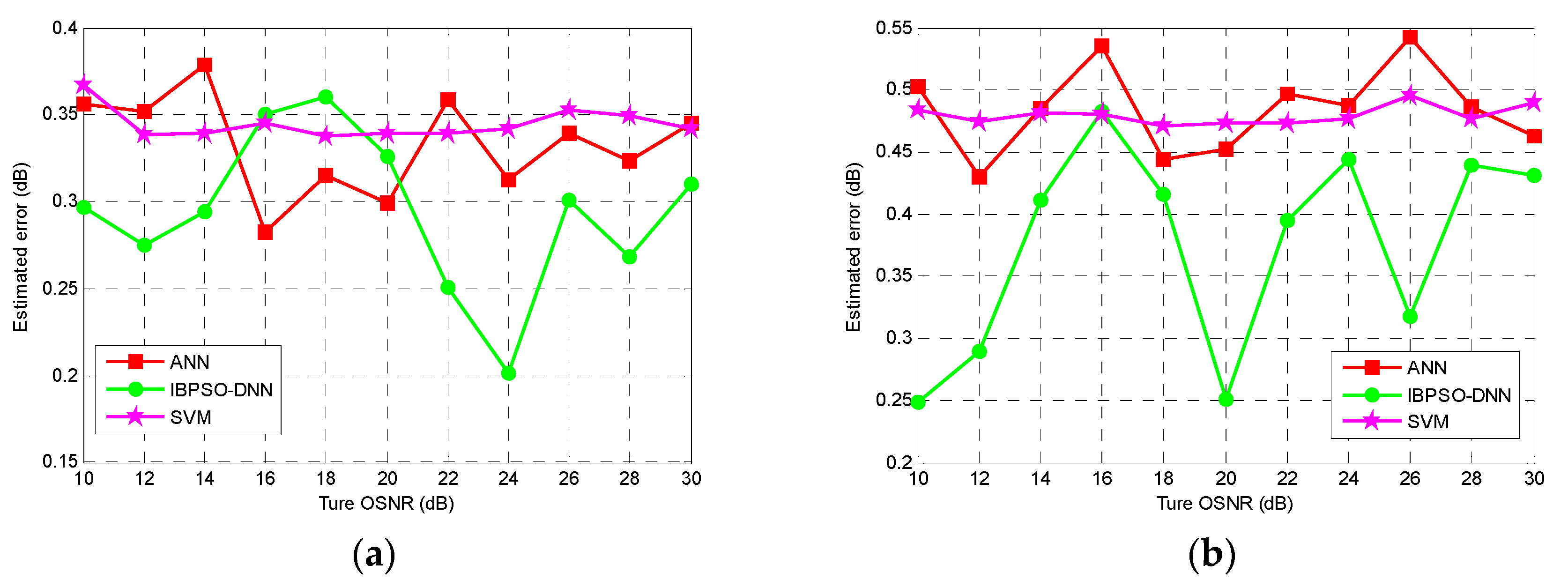
Figure 1. Schematic of the coherent optical receiver and digital signal processing (DSP) for optical signal-to-noise ratio (OSNR) monitoring (LO: local oscillator, PBS: polarization beam splitter, and ADC: analog-to-digital converter).
Photonics 06 00111 g001
Figure 2. Constellation diagrams and amplitude histograms with Fourier fitting at three different OSNRs for PM-RZ-QPSK signals.
Photonics 06 00111 g002
Figure 3. Constellation diagrams and amplitude histograms with Fourier fitting at three different OSNRs for PM-NRZ-16QAM signals.
Photonics 06 00111 g003
Figure 4. Block diagram of deep neural network.
Photonics 06 00111 g004
Figure 5. The flow chart of improved binary particle swarm optimization (IBPSO) algorithm.
Photonics 06 00111 g005
Figure 6. Process of deep neural network (DNN) optimized by IBPSO.
Photonics 06 00111 g006
Figure 7. Experimental setup for OSNR monitoring in coherent receiver.
Photonics 06 00111 g007
Figure 8. Averaged error of estimated OSNR for (a) PM-RZ-QPSK and (b) PM-NRZ-16QAM signals versus AHs bin number processed by the particle swarm optimization optimized deep neural network (PSO-DNN) and DNN.
Photonics 06 00111 g008
Figure 9. The sparse amplitude histogram of (a) PM-RZ-QPSK signal and (b) PM-NRZ-16QAM signal obtained by IBPSO.
Photonics 06 00111 g009
Figure 10. True versus estimated OSNRs and errors for PM-RZ-QPSK signal with (a) 100 bin numbers and (b) 55 bin numbers using PSO-DNN in different OSNRs.
Photonics 06 00111 g010
Figure 11. True versus estimated OSNRs and errors for PM-NRZ-16QAM signal with (a) 100 bin numbers and (b) 65 bin numbers using PSO-DNN in different OSNRs.
Photonics 06 00111 g011aPhotonics 06 00111 g011b
Figure 12. Average estimated errors for (a) PM-RZ-QPSK signal and (b) PM-NRZ-16QAM signal processed by artificial neural network (ANN), improved binary particle swarm optimization and deep neural network (IBPSO-DNN), and support vector machine (SVM).
Photonics 06 00111 g012
Table 1. The average and maximum estimated errors of PM-RZ-QPSK and PM-NRZ-16QAM signals using ANN, IBPSO-DNN, and SVM.
SignalANNIBPSO-DNNSVM
Average/Maximum Error (dB)Average/Maximum Error (dB)Average/Maximum Error (dB)
PM-RZ-QPSK0.33/0.540.29/0.370.34/0.61
PM-NRZ-16QAM0.48/0.650.37/0.480.47/0.72

