Abstract
In-line Fabry–Perot cavities manufactured by a new technique using electric arc fusion of NIR laser microdrilled optical fiber flat tips were studied herein for refractive index sensing. Sensors were produced by creating an initial hole on the tip of a standard single-mode telecommunication optical fiber using a Q-switched Nd:YAG laser. Laser ablation and plasma formation processes created 5 to 10 micron cavities. Then, a standard splicing machine was used to fuse the microdrilled fiber with another one, thus creating cavities with lengths around 100 micrometers. This length has been proven to be necessary to obtain an interferometric signal with good fringe visibility when illuminating it in the C-band. Then, the sensing tip of the fiber, with the resulting air cavity, was submitted to several cleaves to enhance the signal and, therefore, its response as a sensor, with final lengths between tens of centimeters for the longest and hundreds of microns for the shortest. The experimental results were analyzed via two signal analysis techniques, fringe visibility and fast Fourier transform, for comparison purposes. In absolute values, the obtained sensitivities varied between 0.31 nm−1/RIU and about 8 nm−1/RIU using the latter method and between about 34 dB/RIU and 54 dB/RIU when analyzing the fringe visibility.
1. Introduction
Fiber-based Fabry–Perot (FP) interferometers share the advantages of all types of optical fiber sensors: low-cost manufacture, immunity to electromagnetic interference, compact size, and high sensitivity. Some types of FP sensors have the additional advantage of having the sensing head in the tip of the fiber which makes it easier to embed it in small volumes, for example, in biological tissues or even cells for in vivo applications. FP sensors have been developed for a wide range of applications due to their response to different measurands, like temperature, mechanical vibration, voltage, strain, humidity, liquid level, pressure, refraction index, or magnetic field [1,2,3,4,5,6].
FP sensors can have extrinsic or intrinsic cavities, depending on the way in which they are manufactured. While fiber-based extrinsic cavities rely on externally coupled elements to create interference (i.e., the cavity is external to the fiber), for intrinsic sensors the interferometric cavity is created within the fiber (Figure 1). Thus, in an intrinsic FP sensor, the fiber contains the resonant cavity, and it therefore performs as the sensing medium. Different manufacturing methods can be found in the literature, using a few basic principles: creating the cavity on the tip of a fiber and fusing it with another fiber, relying on the creation of microscopic air bubbles embedded in the fiber’s axis [7,8] or air bubbles attached at the end of the fiber or between two fibers, using a glass tube [9,10], or from a photonic bandgap fiber and a polymer [11]. All of them are created with the aid of a fusion splicer. Special photonic fibers have widespread applications, such as the hollow-core fiber [12,13], the use of fillings for creating the cavity itself [12], or the functionalization of the sensor with coatings sensitive to the desired measurand, for example, the pH-sensitive gel in [13]. Another approach is to dig the cavity directly inside the fiber by machining it perpendicularly to the fiber’s axis. Examples can be found in [14], where the fiber is machined with an fs laser to create a notch that performs as a reflection cavity, or in [15], where focused ion beam milling is used. Chemical etching is also widely used to open channels in the fiber, like in [16], allowing the penetration of microfluidics.
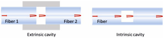
Figure 1.
Schematics of typical extrinsic and intrinsic cavities in Fabry–Perot (FP) fiber-based sensors.
Based on the current state of the art, we present a method to fabricate in-line FP cavities combining laser ablation to machine the fiber, a Q-switched laser emitting in the near infrared (NIR), and a standard splicer machine to create the final cavity. To test these sensors while measuring the refractive index, different interrogation techniques were evaluated. In the next sections we summarize the operation principles behind this family of sensors, describe the experimental procedures, and discuss the obtained performance.
2. Operation Principles
The structure of our sensor is shown in Figure 2. It consists of an air bubble enclosed inside the fiber, forming an in-line FP interferometer. The first and second reflective surfaces are the interfaces of the bubble, making it the first resonant cavity. Their reflection coefficients are, respectively, R1 and R2, and A1, A2 are the transmission coefficients (mainly related with surface imperfections). The second resonant cavity is the one formed between the first and the third reflective surfaces, corresponding the latter to the cleaved end of the fiber. Finally, we consider a third resonant cavity formed by the second and the third reflective surfaces, with R3 and A3 being the reflectance and transmission coefficients for the third reflective surface. The cavity loss factor is identified as α, while ncore and ncladding are the refractive indices of the fiber core and cladding, and n0 represents the refractive index of the surrounding medium. The lengths of cavities 1 and 2 are represented by L1 and L2, and L3 = L1 + L2. The working principle of our sensor is based on the interference between the reflections of the three interfaces. The light intensity of the reflection spectrum of a three-beam interferometer can be expressed as the summation of the intensities of each surface and a term of phase, as described in detail by [17].
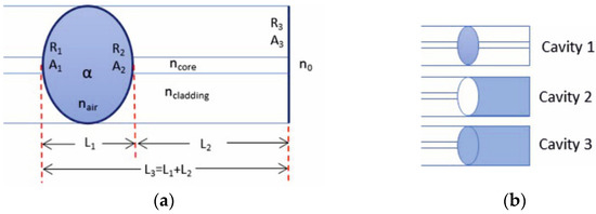
Figure 2.
Schematic representations of the (a) head of the sensor and (b) the three-cavity model.
The response of the FP fiber interferometer to variations in the refractive index of the surrounding medium depends on the reflected intensity, and, therefore, the fringe visibility will be related to the percentage of reflectance (R3) in the tip of the sensor:
where n0 is the refractive index of the medium. When the reflectance R3 increases, the reflected intensity decreases, resulting in a reduction in the optical power and a decrease in the fringe visibility, expressed as
where Imax and Imin are the maximum and minimum intensities recorded in the interferogram, usually corresponding to the highest and lowest peaks of the fringes. The spectral spacing between adjacent interference peaks is known as the free spectral range (FSR) and can be obtained using
where λ02 is the central wavelength of the light with which the interferometer is being illuminated, n is the refraction index within the cavity, L1 is the length of the cavity, and θ is the angle of incidence of the light. It is important to mention that in the present case, it is considered that all the beams fall upon the cavity parallel to the fiber’s axis; as a consequence, the FSR only depends on the wavelength and the cavity length.
3. Experimental Procedures
The sensor manufacturing was previously explained in detail in, for example, [18,19]. The procedure starts with the drilling of a microhole in the optical fiber (SMF-28) flat tip using a Q-switched Nd:YAG laser (Litron TRLI G 450-10) to precisely remove a small portion of the fiber’s glass, with an optical system that focuses the beam onto a small spot, creating a plasma plume when it reaches the tip of the fiber. The same system was used to visualize the drilling process in real time with a CCD camera. The laser operates in the near-infrared (NIR) region with a wavelength of 1064 nm and 60 mJ energy per pulse (pulse width of 6 ns).
The micropatterning process was optimized to obtain the best relation between the number of laser pulses, hole depth and diameter, aspect at the surface, and absence of cracks while avoiding shattering of the fiber. The energy, beam diameter, and focal position were, therefore, carefully chosen [18]. The microstructured fiber was fused to a bare fiber with a splicer machine. The heat produced by the electric discharge expanded the pre-drilled hole, creating a bigger air bubble well trapped within the final fused fiber. The fusion splicer parameters were modified in order to create a cavity without collapsing the previously laser-drilled hole.
In order to tune the interferometer, the length L2 was adjusted (as illustrated in Figure 3) to obtain an interferometric signal with adequate periodicity and visibility by submitting the fiber to successive cleaves, performed manually with a common fiber cleaver, while monitoring the signal with an optical spectrum analyzer (OSA). The contribution of cavities 2 and 3 increases when L2 decreases, resulting in a more complex signal. For simplicity, we limit the description and analysis to two sensors: one with shorter L2, 149 µm, and the other with a much larger length, 22.7 cm (profiting from previous experience in producing strain sensors with this technique [19]), referenced hereafter as “FP-short” and “FP-long”. The values of L1 (and L2 in the case of FP-short) were measured with a microscope, and the longer L2 (for FP-long) was measured with a precision ruler.

Figure 3.
Schematic of the procedure for adjusting L2.
Both sensors were tested for refraction index (RI) variations. The procedure consisted of dipping the FP sensor head into solutions with different RI values, independently measured using a classic non-digital Abbe refractometer. The solutions were prepared by mixing ethylene glycol and distilled water in different concentrations. RI reference values are listed in Table 1. The interrogation system (Figure 4) included an OSA with a resolution of 0.001 dB for monitoring the signal, a light source (a superluminescent diode, SLD, with a central wavelength of 1550 nm), and a three-port optical fiber circulator. Light is coupled into the sensor through Port 1 and goes to the sensor attached to Port 2, and the reflected light is collected and sent to the OSA (Port 3). For each concentration, different spectra were recorded for analysis in the wavelength range between 1500 and 1600 nm, with samples every 0.022 nm and 0.033 nm and 5000 and 1000 data points (FP-short and FP-long, respectively).

Table 1.
Refraction indices used for sensor calibration and their relation to the ethylene glycol concentration.
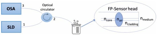
Figure 4.
Interrogation setup for RI sensing. OSA - optical spectrum analyzer; SLD - superluminescent diode.
Based on the type of spectral response of the sensor, two main approaches were tested: one based directly on fringe visibility (Equation (4)) and the other based on signal amplitude spectral analysis (in the k-space), using fast Fourier transform (FFT). The latter was applied to the amplitude signal obtained through the OSA, which corresponded to a sample each 0.008 nm and 2500 data points for the FP-short, and to a sample each 0.001 nm and 500 data points for the FP-long (corresponding to sampling resolutions of 10−6 nm−1). In each case, specific ranges of either wavelength or spectral frequency were defined for obtaining the calibration curves. The criterion for visibility was signal regularity and that for spectral analysis was the existence of well-defined peaks in the Fourier spectral space, after discarding the DC level, related mainly with the source spectral intensity variations. In the defined region of interest for visibility analysis, the maximum and minimum values of intensity were obtained and Equation (4) was applied.
Figure 5 illustrates the outcomes of the three main steps to manufacture the sensors: a typical microphotograph of a laser microdrilled hole (left), a splicer image of the creation of the air bubble (center), and a microphotograph of a cleaved fiber tip. Although depths up to 20 µm are feasible, these microholes are 10 µm deep, a value that has shown good performance in previous manufacturing of FP cavities [18,19]. For the given splicer parameters, the lengths of the final (bubble) cavities were 80 to 100 µm (demonstrating the good repeatability of the method); this provides a wavelength spacing of around 15 to 11 nm, adequate for obtaining good interferogram fringe periodicity according to the FSR calculation (Equation (3)).
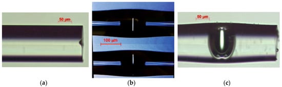
Figure 5.
(a) Microphotograph of a microhole in the optical fiber’s tip, (b) splicer image of the air bubble, obtained just after electric arc discharge, and (c) microscope image of a cleaved FP fiber tip, with L1 = 105 µm and L2 = 149 µm.
4. Results and Discussion
4.1. FP-Short Sensor
Figure 6a shows the reflected spectra for the different RIs, and Figure 6b shows the corresponding spectral amplitudes. For both cases, L1 = 105 µm and L2 = 149 µm. Due to the reduced value of L2, the reflected signal obtained from the OSA has a complex structure and shows irregular fringe spacing due to the three surfaces. Intensity variations can also be observed in the signal, probably due to surface irregularities (mainly in Surface 3) and/or cavity losses. To reduce this effect and the influence of the light source line profile on the calculation of the visibility (Equation (4)), the analysis was restricted to the range 1530 nm to 1560 nm (rectangle in Figure 6a). Figure 7 shows the derived linear regression between the visibility and the RI for this approach, which can be used as the calibration curve. A sensitivity of −34.267 dB/RIU was obtained with a coefficient of determination, R2, of 92.7%.
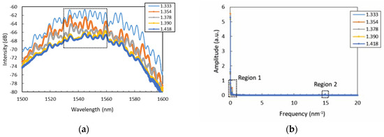
Figure 6.
(a) Reflected signal for the FP-short sensor (L1 = 105 µm and L2 = 149 µm) and (b) the resulting spectral analysis.
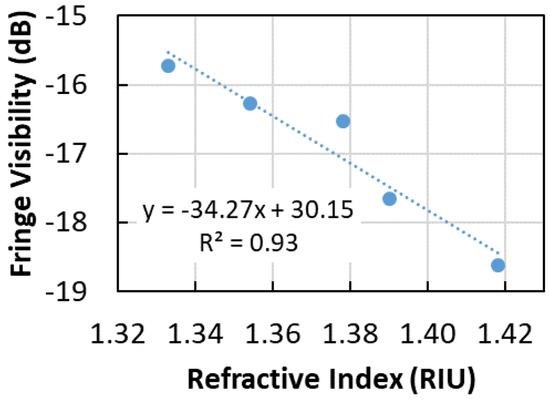
Figure 7.
Calibration curve for the FP-short sensor (L1 = 105 µm and L2 = 149 µm) using signal visibility in the range 1530 nm to 1560 nm.
Regarding the FFT analysis of the original spectrum, two relevant regions can be seen in Figure 6b: one for spatial frequency below 0.5 nm−1 and the other in the range 12.5 nm−1 to 16 nm−1. These regions can be analyzed in more detail in Figure 8, zooming the regions of interest from Figure 6b. It becomes clear that only in Region 2 are there amplitude changes with the RI in the four peaks identified. Linear regression was set up between the peaks’ amplitude and RI (or calibration curves, in Figure 9), and although the best sensitivity was obtained from Peak 3 (0.31 dB/RIU with R2 = 93%), the best fit corresponded to Peak 2 (0.15 dB/RIU with R2 = 98%).
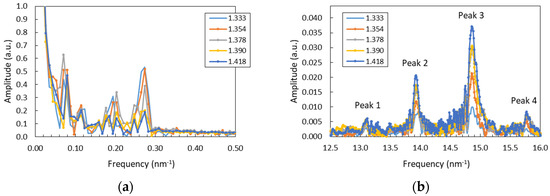
Figure 8.
Spatial frequency amplitude plots for the two regions in the spectral analysis for the FP-short sensor (L1 = 105 µm and L2 = 149 µm): (a) 0.01 nm−1 to 0.5 nm−1 and (b) 12.5 nm−1 to 16 nm−1. Each plot represents a zoom of one of the two regions in Figure 6b.
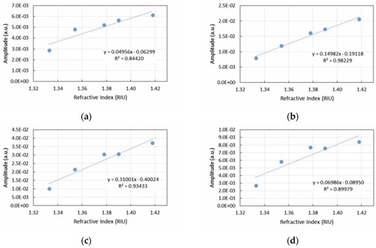
Figure 9.
Calibration curves for the FP-short sensor (L1 = 105 µm and L2 = 149 µm) using spectral analysis and considering Peaks (a) 1, (b) 2, (c) 3, and (d) 4 with regard to Figure 8b.
4.2. FP-Long Sensor
For the FP-long sensor, L1 = 80 µm and L2 = 22.7 cm. The analysis is similar to that for the FP-short case. Figure 10a shows the reflected signal, and Figure 11 shows the corresponding linear regressions between the signal modulation visibility and wavelength made independently for Regions 1 and 2, as sketched in Figure 10a. Sensitivities can be derived from the regression plots in Figure 11. For Region 1, between 1536 and 1539 nm, R2 = 99% and the sensitivity was −54.2 dB/RIU. For Region 2, between 1552 and 1555 nm, R2 = 90.5% and the sensitivity was −50.1 dB/RIU.
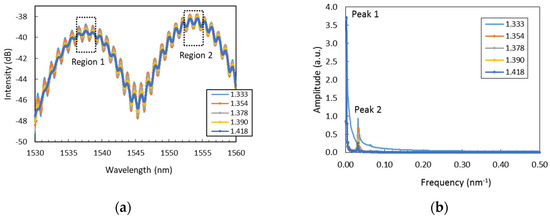
Figure 10.
(a) Reflected signal for the FP-long sensor (L1 = 80 µm and L2 = 22.7 cm) and (b) the resulting spectral analysis. Analysis was restricted to the wavelength ranges associated with the dotted rectangles.
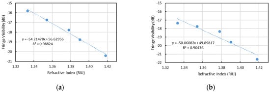
Figure 11.
Calibration curve for the FP-long sensor (L1 = 80 µm and L2 = 22.7 cm) using the signal modulation visibility for wavelength ranges (a) 1536 nm to 1539 nm and (b) 1552 nm to 1555 nm.
Regarding the spectral analysis using the FFT (Figure 10b), Figure 12b shows that only the large spatial frequency peak (from 0.025 nm−1 to 0.045 nm−1) is relevant because the spectral amplitude can be correlated with the RI. In Figure 12a, all curves are identical with the exception of the curve for RI = 1.333. Linear regression was therefore set up only for Peak 2, and this is shown in Figure 13: the estimated sensitivity was −7.92 nm−1/RIU for R2 = 94%.
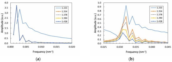
Figure 12.
Frequency amplitude plots within the peaks considered for spectral analysis of the FP-long sensor (L1 = 80 µm and L2 = 22.7 cm): (a) Peak 1 and (b) Peak 2.
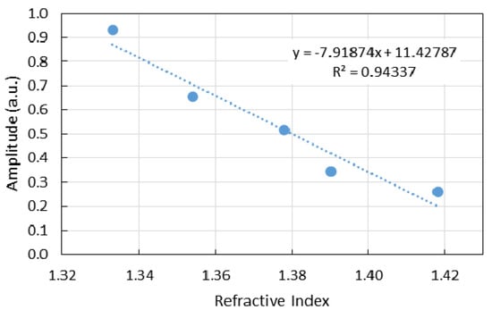
Figure 13.
Calibration curve of the FP-long sensor (L1 = 80 µm and L2 = 22.7 cm) using the spectral analysis restricted to Peak 2.
4.3. Discussion
Table 2 presents the data obtained for both sensors using the two approaches—visibility analysis and spectral amplitude using wavenumber differences—in terms of sensitivity and the quality of the linear regression with RI. Similarly, Table 3 allows us to compare the differences between the calibration values and those obtained using the sensors (percent error). Although the sensitivity analysis regarding the two interrogation techniques cannot be compared directly (one is in dB/RIU and the other in nm−1/RIU), the two can be evaluated by considering the easiness of interrogation and the coefficient of determination associated with calibration. The calibration equations have high R2 values independent of the type of sensor or method. Nevertheless, for the FP-short sensor, the FFT analysis allows a better fit (and lower deviation from the calibration values), although with a lower sensitivity. This type of sensor, where the first and second resonant cavities (Figure 2) have similar lengths (i.e., the same order of magnitude), has a signal with more irregular fringe spacing and with a mixture of different frequencies or beats due to multiple interferences and phase mismatch. This results in the observed lower fringe visibility and lower amplitude for the FFT analysis. Also, as a consequence of the high level of fringe irregularity, the definition of the region where the fringe visibility will be determined is critical for FP-short sensors.
Table 2.
Results of the sensitivity analysis. Values are approximated.
Table 3.
Results of the differences between refractive indices obtained through calibration (Abbe refractometer) and those obtained from the FP sensors.
Regarding the FP-long sensor, its signal shows regular, high-visibility fringes. On the two wavelength regions considered (Figure 10a), the sensitivity is similar, although the calibration equation results in better fitting (and a smaller difference between measurements and calibration data). From the two main peaks identified on the FFT analysis, only the one corresponding to higher special frequencies (Peak 2; range 0.025 nm−1 to 0.045 nm−1) showed sensitivity to refractive index changes. In this case, the sensitivity was much higher than that observed for the same analysis method on the FP-short sensor. However, the fitting had a slightly lower R2 value, especially when comparing the results from the second peaks on each sensor. Comparing the plots in Figure 8 and Figure 12, this lower fitting can be explained by a resolution of insufficient frequency. Considering that the resolution of the OSA used is 0.001 dB, the resolution in measuring the refractive index using the fringe visibility method lies between 3 × 10⁻⁵ and 2 × 10⁻⁵, depending on the sensor and region of interest. So, regarding this analysis method, the RI resolution can be considered as not having a major dependency on the type of sensor. For the FFT method, using the sampling resolution (Section 1), the obtained resolution in measuring the refractive index lies between 7 × 10⁻⁶ (FP-short, Peak 2) and 1 × 10⁻⁷ (FP-long, Peak 2).
On both sensors, two main frequencies were presented. Measuring directly from each signal, the FSR can be used to determine the corresponding cavity lengths (Equation (3)). Regarding the lower frequencies, the calculated values for FP-short and FP-long were around 110 µm (FSR = 10.91 nm) and 77 µm (FSR = 15.65 nm), respectively. These values are in agreement with the measured bubble lengths (L1) considering the uncertainties of the measurements, particularly the irregularities on the FP-short signal. However, when calculating for the higher frequencies, while the values for FP-short were consistent with the second cavity length (L2)—around 200 µm (FSR = 4 nm)—the values calculated for the FP-long were around 832 µm (FSR = 1 nm), far shorter than the measured length. So far, we do not have an explanation for this cavity length obtained from FSR measurement. Future work will focus on this subject. Nevertheless, it was observed experimentally that if L2 is large enough, the interferogram shows more regular fringe spacing and periodicity, and it is hypothesized that it can then be considered a two-beam interferometer wherein the contributions of Cavities 2 and 3 are negligible. When L2 is small, the contributions of Cavities 2 and 3 cannot be discarded, as a more complex interferogram is observed. In the latter case, the difficulty of analyzing the obtained interferograms makes the FFT technique more suitable for interrogating our FP sensor because they usually show irregular fringe spacing, with a mixture of different frequencies or beats due to multiple interferences and phase mismatch. Carefully choosing the region for analysis has proven able to overcome this issue but might be operationally less practical. In contrast, smaller sensor heads are easier to manipulate and less influenced by cross sensitivity to mechanical deformations like strain or bending during the measurements. Besides this, to improve the refractive index measurement calibration it will be necessary to use a wider range of solutions, preferably calibration standards, avoiding eventual imprecision induced by measurement with the Abbe refractometer. This is important to the uncertainty associated with calibration being reduced and the full potential resolution of the sensor being achieved.
5. Conclusions
In this paper we presented a method for manufacturing in-line fiber Fabry–Perot cavities based on microstructured optical fiber flat tips. The preliminary drilling was performed using an NIR Q-switched Nd:YAG laser to obtain microholes that result in embedded air bubbles along the fiber axis. A splicer machine was used to fuse a bare fiber with a microstructured one. The heat of the electric arc discharge expanded the microhole, creating an air cavity big enough to function as an FP interferometer. Two sensors with different tip lengths were then created. The resulting FP cavities were tested for refraction index measurement, obtaining sensitivities with absolute value of up to about 8 nm−1/RIU for amplitude variations in in the frequency space when analyzed using FFT. Direct measurements, like tracking the variation of the fringe visibility in the interferogram, resulted in a more complicated and less reliable method of interrogation, since the obtained interferograms were usually irregular (particularly for the short-tip sensor) with superposed frequencies and beats. Nevertheless, sensitivities with absolute values up to about 54 dB/RIU were accomplished, depending on the spectral range chosen for analysis.
These kinds of sensors have proved to be easy to manufacture and with high repeatability regarding cavity dimensions. The use of NIR laser pulses to predefine the cavity and electric arc fusion to finalize the sensor proved to be a reliable and inexpensive method to create this kind of sensor when compared with femtosecond laser machining fabrication or the use of different types of photonic crystal fibers. As shown, its application as a refractive index sensor proved to be effective, although a few points still need further research. Besides improving the methodologies and better understanding some of the unexpected phenomena that were mentioned, future work will be directed toward making the most of the flexibility that the microstructuring offers to open channels in the cavities to allow different fills. The possibility of increasing the reflectivity of the cavity’s surfaces will be explored, as well as the creation of different structures with the splicer, like bulk microspheres in the tip of the sensor head.
Author Contributions
Conceptualization, M.N., J.M.P.C. and J.M.R.; methodology, M.N. and J.M.P.C.; formal analysis, M.N. and J.M.P.C.; writing—original draft preparation, M.N.; writing—review and editing, M.N., J.M.P.C. and J.M.R.; supervision, J.M.P.C. and J.M.R.
Funding
This research was partially funded by Fundação para a Ciência e Tecnologia (FCT), grant number UID/BIO/00645/2019.
Conflicts of Interest
The authors declare no conflict of interest.
References
- Islam, M.; Ali, M.; Lai, M.H.; Lim, K.S.; Ahmad, H. Chronology of Fabry-Perot interferometer fiber-optic sensors and their applications: A review. Sensors 2014, 14, 7451–7488. [Google Scholar] [CrossRef] [PubMed]
- Javernik, A.; Donlagic, D. Miniature, micro-machined, fiber-optic Fabry-Perot voltage sensor. Opt. Express 2019, 27, 13280–13291. [Google Scholar] [CrossRef] [PubMed]
- Liang, H.; Jia, P.; Liu, J.; Fang, G.; Li, Z.; Hong, Y.; Liang, T.; Xiong, J. Diaphragm-Free Fiber-Optic Fabry-Perot Interferometric Gas Pressure Sensor for High Temperature Application. Sensors 2018, 18, 1011. [Google Scholar] [CrossRef] [PubMed]
- Cheng, J.; Zhou, Y.; Zou, X. Fabry-Perot Cavity Sensing Probe with High Thermal Stability for an Acoustic Sensor by Structure Compensation. Sensors 2018, 18, 3393. [Google Scholar] [CrossRef] [PubMed]
- Flores, R.; Janeiro, R.; Viegas, J. Optical fibre Fabry-Pérot interferometer based on inline microcavities for salinity and temperature sensing. Sci. Rep. 2019, 9, 9556. [Google Scholar] [CrossRef] [PubMed]
- Budinski, V.; Donlagic, D.A. Miniature Fabry Perot Sensor for Twist/Rotation, Strain and Temperature Measurements Based on a Four-Core Fiber. Sensors 2019, 19, 1574. [Google Scholar] [CrossRef] [PubMed]
- Liao, C.R.; Hu, T.Y.; Wang, D.N. Optical fiber Fabry-Perot interferometer cavity fabricated by femtosecond laser micromachining and fusion splicing for refractive index sensing. Opt. Express 2012, 20, 22813–22818. [Google Scholar] [CrossRef] [PubMed]
- Duan, D.W.; Rao, Y.J.; Hou, Y.S.; Zhu, T. Microbubble based fiber-optic Fabry–Perot interferometer formed by fusion splicing single-mode fibers for strain measurement. Appl. Opt. 2012, 51, 1033–1036. [Google Scholar] [CrossRef] [PubMed]
- Yan, L.; Gui, Z.; Wang, G.; An, Y.; Gu, J.; Zhang, M.; Liu, X.; Wang, Z.; Wang, G.; Jia, P. A micro bubble structure based Fabry–Perot optical fiber strain sensor with high sensitivity and low-cost characteristics. Sensors 2017, 17, 555. [Google Scholar] [CrossRef] [PubMed]
- Monteiro, C.S.; Ferreira, M.S.; Silva, S.O.; Kobelke, J.; Schuster, K.; Bierlich, J.; Frazão, O. Fiber Fabry-Perot interferometer for curvature sensing. Photonic Sens. 2016, 6, 339–344. [Google Scholar] [CrossRef]
- Tan, X.; Li, X.; Geng, Y.; Yin, Z.; Wang, L.; Wang, W.; Deng, Y. Polymer microbubble-based Fabry–Perot fiber interferometer and sensing applications. IEEE Photonic Technol. Lett. 2015, 27, 2035–2038. [Google Scholar] [CrossRef]
- Chen, M.Q.; Zhao, Y.; Xia, F.; Peng, Y.; Tong, R.J. High sensitivity temperature sensor based on fiber air-microbubble Fabry-Perot interferometer with PDMS-filled hollow-core fiber. Sens. Actuator A Phys. 2018, 275, 60–66. [Google Scholar] [CrossRef]
- Zheng, Y.; Chen, L.H.; Dong, X.; Yang, J.; Long, H.Y.; So, P.L.; Chan, C.C. Miniature pH optical fiber sensor based on Fabry–Perot interferometer. IEEE J. Sel. Top. Quantum Electron. 2015, 22, 331–335. [Google Scholar] [CrossRef]
- Tian, M.; Lu, P.; Chen, L.; Liu, D.; Yang, M.; Zhang, J. Femtosecond laser fabricated in-line micro multicavity fiber FP interferometers sensor. Opt. Commun. 2014, 316, 80–85. [Google Scholar] [CrossRef]
- Warren-Smith, S.C.; André, R.M.; Dellith, J.; Eschrich, T.; Becker, M.; Bartelt, H. Sensing with ultra-short Fabry-Perot cavities written into optical micro-fibers. Sens. Actuator B Chem. 2017, 244, 1016–1021. [Google Scholar] [CrossRef]
- Wu, S.; Yan, G.; Zhou, B.; Lee, E.H.; He, S. Open-cavity fabry-perot interferometer based on etched side-hole fiber for microfluidic sensing. IEEE Photonics Technol. Lett. 2015, 27, 1813–1816. [Google Scholar]
- Ran, Z.L.; Rao, Y.J.; Liu, W.J.; Liao, X.; Chiang, K.S. Laser-micromachined Fabry-Perot optical fiber tip sensor for high-resolution temperature-independent measurement of refractive index. Opt. Express 2018, 16, 2252–2263. [Google Scholar] [CrossRef] [PubMed]
- Nespereira, M.; Silva, C.; Coelho, J.; Rebordão, J. Nanosecond laser micropatterning of optical fibers. In Proceedings of the International Conference on Applications of Optics and Photonics, Braga, Portugal, 3–7 May 2011; Volume 8001, p. 800140. [Google Scholar]
- Nespereira, M.; Coelho, J.; Rebordão, J. In line Fabry-Perot cavities manufactured by electric arc fusion of NIR-laser micro-drilled optical fiber flat tips. In Proceedings of the Fourth International Conference on Applications of Optics and Photonics, Lisbon, Portugal, 31 May–4 June 2019; Volume 11207, p. 112072F. [Google Scholar]


© 2019 by the authors. Licensee MDPI, Basel, Switzerland. This article is an open access article distributed under the terms and conditions of the Creative Commons Attribution (CC BY) license (http://creativecommons.org/licenses/by/4.0/).