Photonic Time-Stretch Technology with Prismatic Pulse Dispersion towards Fast Real-Time Measurements

Abstract

Photonic time-stretch (PTS) technology enables revolutionary technical breakthroughs in ultrafast electronic and optical systems. By means of employing large chromatic dispersion to map the spectrum of an ultrashort optical pulse into a stretched time-domain waveform (namely, using the dispersive Fourier transformation), PTS overcomes the fundamental speed limitations of conventional techniques. The chromatic dispersion utilized in PTS can be implemented using multiple optical prism arrays, which have the particular advantages of low loss in the extended spectrum outside of the specific telecommunication band, flexibility, and cost-effectiveness. In this article, we propose and demonstrate the PTS technology established for a pair of prisms, which works as a data acquisition approach in ultrafast digitizing, imaging, and measurement regimes.

1. Introduction

In digital signal processing (DSP), the data consists of finite samples of discrete values, derived from a practically continuous physical system [1,2]. Implemented by a digital signal processor or a similarly capable device, DSP plays an indispensable role in the development of the electronics industry and modern communications systems [3]. However, limited bandwidth (speed) is a major bottleneck hampering the progress of DSP towards higher rates and resolutions, which leads to only average signal behavior information being provided [2,4]. One potential solution for tackling this electronic barrier is the use of photonic preprocessing [5]. Therefore, diverse attractive photonic techniques have been actively researched and developed to boost and enhance the performance of conventional DSP systems [6,7,8]. With its distinct attributes of sufficiently large optical bandwidth and immunity to channel-to-channel crosstalk, photonic DSP is capable of acquiring ultra-fast pulses and achieving analog-to-digital conversion of wideband electrical signals.

Photonic time-stretch (PTS) is a promising approach to address the inherent drawbacks of the available electronic DSP systems, which has shown benefits in measurement and in understanding the behaviour of ultrafast phenomena [9,10,11]. The most fundamental part of the PTS is the dispersive Fourier transformation (DFT), also referred as the frequency-to-time mapping, which utilizes a large chromatic dispersion to map the spectrum of an optical pulse to a temporal waveform [12,13,14]. Concurrently, the analog signal is optically slowed down, prior to sampling and quantization by an electronic digitizer, which mimics the optical power spectrum of the initial optical pulse [10,15]. To date, PTS has become a widespread and rapidly evolving tool and has been used a variety of different applications, such as wideband analog-to-digital converters (ADC) [7,16], continuous ultrafast single-shot images [17,18], real-time spectroscopy [19,20], and many more.

The most common way to realize the DFT procedure is by using dispersion-compensating fibers (DCF) as a dispersive optical element, aimed at controlling the overall chromatic dispersion of PTS system [21,22]. However, the utility of PTS is typically restrained at the 1.5 $\mathsf{\mu }$m telecommunication band, as larger dispersion comes at the expense of higher losses in other spectral bands, especially in the infrared band [23,24,25,26]. For instance, the fiber transmission attenuation at 2.0 $\mathsf{\mu }$m is approximately 30 dB/km, which inevitably deteriorates the efficiency of PTS systems [25,27]. As a consequence, alternative dispersive devices for implementing PTS with sufficient chromatic dispersion and low loss in the infrared band are extremely desirable [28].

Prims have been of great interest since the first description of multiple-prism dispersion given by Newton in his book Opticks [29], and have the ability to generate controllable prismatic dispersion through light refraction [30,31]. Hence, the usage of prisms as dispersive elements has played a significant and indispensible role in the optical regime, such as the use of a two-prism arrangement in a laser pulse compressor and expander in [32,33,34]. In addition, the peculiar merits of multiple-prism systems, generally creating negative group-velocity dispersion, include low insertion loss, ease of adjusting, and mitigation of transverse displacement of temporally dispersed beams [35,36]. For this reason, the multiple-prism approach shows great potential for implementing PTS processes with large and uniform chromatic dispersion, which is essentially required in DFT.

In this article, we discuss the fundamental and practical considerations of a PTS system featuring a dispersive prism pair, which is required to expand the spectral band of a conventional PTS system. Section 2 characterizes the elementary dispersive properties of the optical prisms in detail. In Section 3, the operating principles of the DFT procedure using a two-prism architecture, the core of the PTS technology, is described and explained. Demonstration of various typical applications of prism-based PTS is carried out and reported in Section 4. Section 5 provides a discussion of the high-order dispersion induced by multiple prisms, which most likely impacts on the performance of PTS. Furthermore, new infrared optical materials with proper refractive index dispersion, which are expected to optimize the configuration of the prism-based PTS, are also described and presented. Ultimately, we summarize and conclude our work in Section 6.

2. Dispersive Properties of Prisms

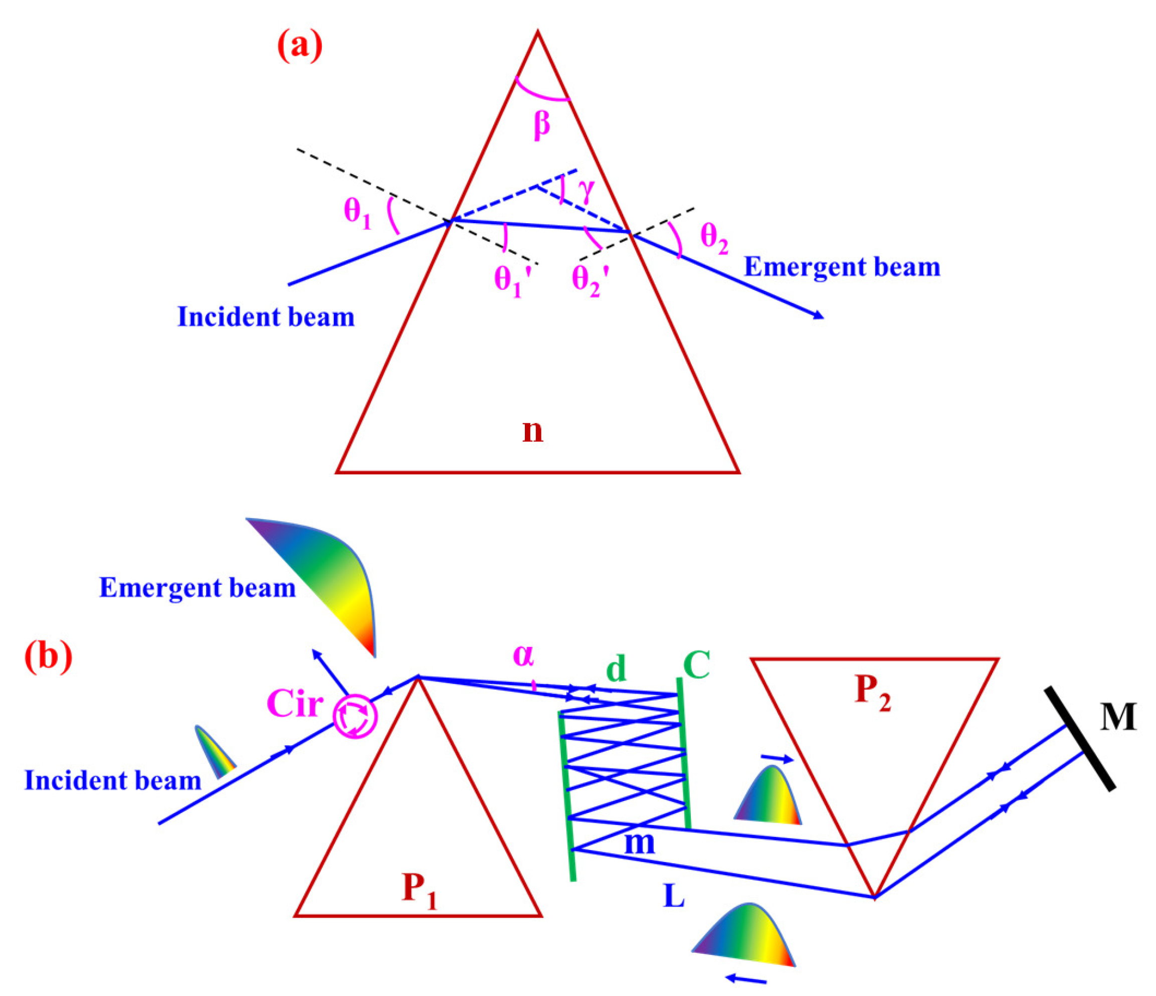
A modern two-prism array, as a potential beam expanding and pulse stretching strategy for a PTS system, is presented in this Section [37,38]. Positive refraction of a single prism is illustrated in Figure 1a, where the prismatic equations become

$$\begin{array}{cc}\hfill {\theta }_1+{\theta }_2& =\beta +\gamma \hfill \end{array}$$

(1)

$$\begin{array}{cc}\hfill {\theta }_1^{\prime }+{\theta }_2^{\prime }& =\beta ,\hfill \end{array}$$

(2)

where ${\theta }_1$ and ${\theta }_2$ represent the incident angle and output angle, respectively, and ${\theta }_1^{\prime }$ and ${\theta }_2^{\prime }$ represent the corresponding refraction angles. In addition, the prism apex angle is $\beta$ and the angle between the emergent and incident beam is defined as $\gamma$.

From Snell’s law, we have

$$\begin{array}{cc}\hfill sin{\theta }_1& =nsin{\theta }_1^{\prime }\hfill \end{array}$$

(3)

$$\begin{array}{cc}\hfill sin{\theta }_2& =nsin{\theta }_2^{\prime },\hfill \end{array}$$

(4)

where n is the refraction index of the prism.

Figure 1b exhibits the two-prism configuration for PTS using negative dispersion, mainly consisting of two prisms, a cavity, and a reflective mirror. The single prism is shaped as an isosceles triangle with high transmission efficiency. Note that the entrance face of prism $P_2$ is parallel to the exit face of prism $P_1$, and the exit face of prism $P_2$ is parallel to the entrance of prism $P_1$. Getting rid of the spatial dispersion requires propagation through an additional identical prism pair, which is realized by setting the pulse back to original prism pair to compensate for spatial dispersion and correct the pulse-front tilt. We place a collimator in front of prism P${}_1$ to reduce the divergence of the input beam and effectively eliminate the astigmatism. The mirror M used for reflecting back the beam light is coated with protected gold, which has 99.9% reflectivity in the band of 0.8–10 $\mathsf{\mu }$m. In addition, one free-space circulator is introduced into the two-prism configuration, to separate the incident and emergent beams in the same path [39].

For the sake of reducing the overall volume of the prism pair to a great extent, a cavity is intentionally introduced to increase the light propagation distance and generate sufficient chromatic dispersion. The cavity is mainly comprised of two metal mirrors coated with protected silver, which provide a high reflectivity (99.8%) and a wide bandwidth range (from 0.4–10 $\mathsf{\mu }$m). There also exists a tiny angle $\tau$ between the two mirror surfaces ($\tau$ = 0.2–3 mrad), whose attainable goal is compressing the beam divergence when light propagates in the cavity. Considering the requirement of miniaturizing the proposed system, the round-trip number in the cavity is fixed at 100. By adjusting the separation distance d between two reflective mirrors of cavity, from 0–0.5 m, the total propagation distance L ranges from 0–50 m with approximately 1 dB of transmission loss.

$$tan{\theta }_1=tan{\theta }_2=n$$

(5)

The first and second derivatives of the output angle, with respect to wavelength, are given by

$$\begin{array}{cc}\hfill \frac{\partial {\theta }_2}{\partial \lambda }& =\frac{\partial {\theta }_2}{\partial n}\frac{dn}{d\lambda }\hfill \end{array}$$

(6)

$$\begin{array}{cc}\hfill \frac{{\partial }^2{\theta }_2}{\partial {\lambda }^2}& =\frac{{\partial }^2{\theta }_2}{\partial n^2}{(\frac{dn}{d\lambda })}^2+\frac{\partial {\theta }_2}{\partial n}\frac{d^{2}n}{d{\lambda }^2},\hfill \end{array}$$

(7)

where

$$\begin{array}{cc}\hfill \frac{\partial {\theta }_2}{\partial n}& =\frac{sin{\theta }_2^{\prime }+cos{\theta }_2^{\prime }tan{\theta }_1^{\prime }}{cos{\theta }_2}\hfill \end{array}$$

(8)

$$\begin{array}{cc}\hfill \frac{{\partial }^2{\theta }_2}{\partial n^2}& =tan{\theta }_2{(\frac{\partial {\theta }_2}{\partial n})}^2-\frac{{tan}^2{\theta }_1^{\prime }}{n}(\frac{\partial {\theta }_2}{\partial n}).\hfill \end{array}$$

(9)

When the prism is used at minimum deviation and Brewster’s angle, Equations (8) and (9) can be simplified to

$$\begin{array}{cc}\hfill \frac{\partial {\theta }_2}{\partial n}& =2\hfill \end{array}$$

(10)

$$\begin{array}{cc}\hfill \frac{{\partial }^2{\theta }_2}{\partial n^2}& =4n-\frac{2}{n^3}.\hfill \end{array}$$

(11)

On the other hand, the center rays of the various wavelengths define a propagation angle $\alpha (\omega )$, and the total optical path that contributes to the dispersion is

$$P=2Lcos\alpha .$$

(12)

As $\alpha$ is defined in the opposite sense, compared to ${\theta }_2$, we have

$$\frac{\partial \alpha }{\partial \lambda }=-\frac{\partial {\theta }_2}{\partial \lambda }.$$

(13)

The derivatives of the length P relative to the wavelength are of the form

$$\begin{array}{cc}\hfill \frac{\partial P}{\partial \lambda }& =L(cos\alpha -sin\alpha (\frac{\partial \alpha }{\partial \lambda }))\hfill \end{array}$$

(14)

$$\begin{array}{cc}\hfill \frac{{\partial }^{2}P}{\partial {\lambda }^2}& =-L(cos\alpha {(\frac{\partial \alpha }{\partial \lambda })}^2+sin\alpha (\frac{{\partial }^2\alpha }{\partial {\lambda }^2}))\hfill \end{array}$$

(15)

In view of the relationship $\omega =\frac{2\pi c}{\lambda }$, the second-order phase dispersion is given by

$$\frac{{\partial }^2\psi }{\partial {\omega }^2}=\frac{-{\lambda }^3}{2\pi c^2}\frac{{\partial }^{2}P}{\partial {\lambda }^2}.$$

(16)

Substituting Equation (15) in Equation (16), we find

$$\frac{{\partial }^2\psi }{\partial {\omega }^2}=\frac{2{\lambda }^{3}L}{\pi c^2}[2cos\alpha {(\frac{dn}{d\lambda })}^2-sin\alpha (\frac{d^{2}n}{d{\lambda }^2}+(2n-\frac{1}{n^3}){(\frac{dn}{d\lambda })}^2)].$$

(17)

On the basis of the known relationship $\psi (\omega )=-\beta L$, the second-order dispersion coefficient can be expressed as

$${\beta }_2=-\frac{{\partial }^2\psi (\omega )}{{\partial }^2\omega }·\frac{1}{L}=\frac{2{\lambda }^3}{\pi c^2}[2cos\alpha {(\frac{dn}{d\lambda })}^2-sin\alpha (\frac{d^{2}n}{d{\lambda }^2}+(2n-\frac{1}{n^3}){(\frac{dn}{d\lambda })}^2)].$$

(18)

The dispersion constant is based on the mathematic relationship $D=-\frac{2\pi c}{{\lambda }^2}{\beta }_2$ and the double-pass configuration, with the resultant dispersion constant of the form

$$D=\frac{4\lambda }{c}[-2cos\alpha {(\frac{dn}{d\lambda })}^2+sin\alpha (\frac{d^{2}n}{d{\lambda }^2}+(2n-\frac{1}{n^3}){(\frac{dn}{d\lambda })}^2)].$$

(19)

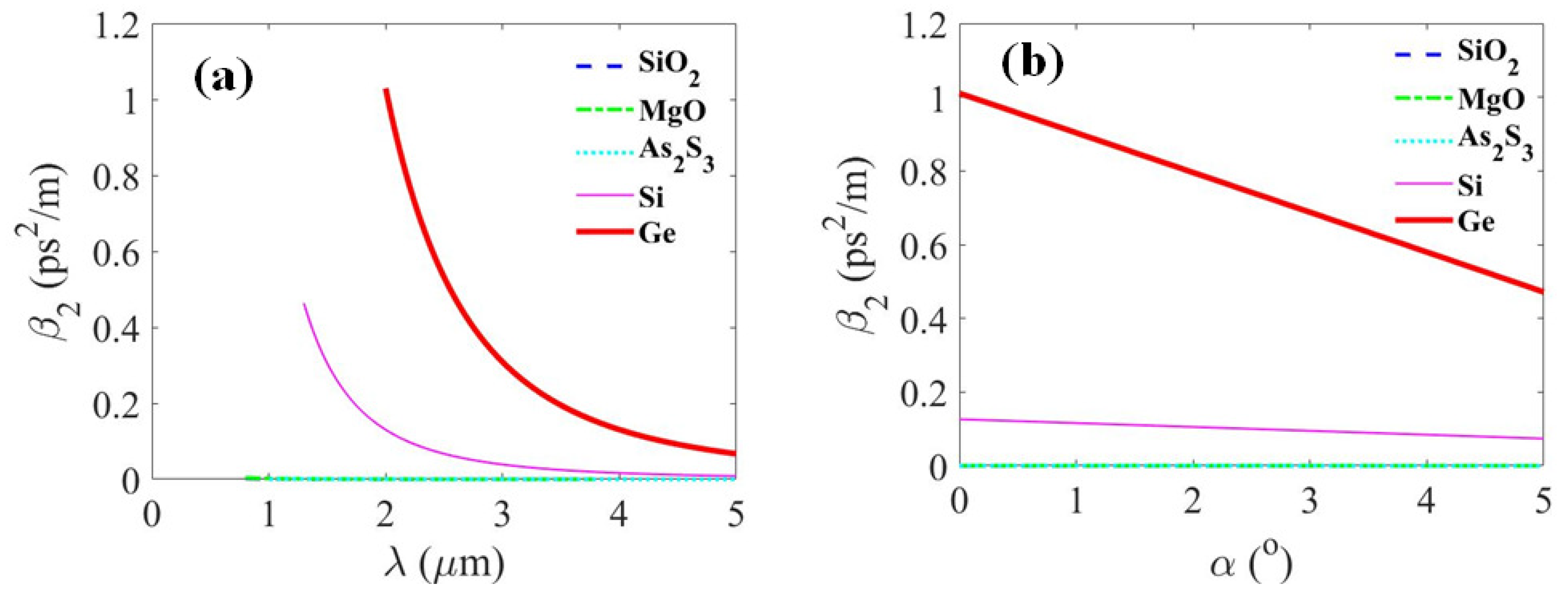
Taking a typical infrared material as an example, the dispersive properties of SiO${}_2$, MgO, As${}_2$S${}_3$, Si, and Ge are depicted in Figure 2. Material dispersion curves are obtained from dispersion formulas in the 0.8–5 $\mathsf{\mu }$m range [40]. Referring to Figure 3, the second-order dispersion coefficients are calculated and plotted with various infrared materials, as the light wavelength $\lambda$ and propagation angle $\alpha$ are varied. Figure 4 shows the simulated results of the dispersion constant in the infrared band, which indicate that the materials Si and Ge are capable of providing sufficient dispersion for PTS applications.

When traveling through the prism pair configuration, the time-wavelength transformation is controlled by the dispersion properties. The group delay can be described as

$$\tau (\lambda )=\int Dd\lambda =\int \frac{4\lambda }{c}[-2cos\alpha {(\frac{dn}{d\lambda })}^2+sin\alpha (\frac{d^{2}n}{d{\lambda }^2}+(2n-\frac{1}{n^3}){(\frac{dn}{d\lambda })}^2)]d\lambda .$$

(20)

On the other hand, the time duration into which the laser spectrum is mapped can be calculated as

$$\Delta \tau =|D|L\Delta \lambda .$$

(21)

In the following parts of this article, we assume all prism pairs are comprised of Ge material and that the operation band is set around 2 $\mathsf{\mu }$m to optimize the experimental configuration. Considering the largest propagation distance (L = 50 m), the achieved maximum dispersion constant D and second-order dispersion coefficient ${\beta }_2$ are −25 ps/nm and 50 ps${}^2$, respectively.

3. Dispersive Fourier Transformation with Prism Pair

In this section, the prism pair is modeled as a dispersive element to implement the DFT for optical light [13,21,41]. Assume that $x(t)$ and $y(t)$ represent the complex envelopes of the input and output optical pulses of a dispersive element with an impulse response $h(t)$, respectively. When the bandwidth of the utilized prism pair covers the entire spectrum of the input pulse, the relationship between envelopes of $x(t)$ and $y(t)$ becomes

$$y(t)=x(t)\ast h(t).$$

(22)

The prism pair can be modeled as a linear time-invariant system with transfer function

$$H(\omega )=|H(\omega )|exp(-i\mathsf{\Phi }(\omega )),$$

(23)

where $|H(\omega )|$ and $\varphi (\omega )$ are the magnitude and phase response of the dispersive element at angular frequency $\omega$, respectively. Mathematically, the phase response $\varphi (\omega )$ is the Taylor series. Under the second-order dispersion approximation, the transfer function and the corresponding impluse response of the dispersive element is given by

$$h(t)=F^{-1}(H(\omega ))\propto exp(\frac{i{(t-\dot{\varphi })}^2}{2\ddot{\varphi }}),$$

(24)

where $\varphi$ represents the group delay and $\ddot{\varphi }$ represents the second-order dispersion, also referred as group velocity dispersion (GVD), which has the mathematical form

$$\ddot{\varphi }=-\frac{\partial \varphi {(\omega )}^2}{\partial {\omega }^2}.$$

(25)

Therefore, the output pulse can be rewritten as

$$\begin{array}{cc}\hfill y(t)& =C{\int }_{-\infty }^{\infty }x(t^{\prime })h(t-t^{\prime })d{t}^{\prime }\hfill \\ & =C{\int }_{-\infty }^{\infty }x(t^{\prime })\exp (\frac{i{(t-t^{\prime })}^2}{2\ddot{\varphi }})\hfill \\ & \hfill =Cexp(\frac{i{t}^2}{2\ddot{\varphi }}){\int }_{-\infty }^{\infty }x(t^{\prime })exp(\frac{i{t}^{\prime 2}}{2\ddot{\varphi }})exp(\frac{-it{t}^{\prime }}{\ddot{\varphi }})d{t}^{\prime },\end{array}$$

(26)

where C denotes a constant time and $t^{\prime }$ is the integral variable. If $x(t)$ is confined to a small time bandwidth $\Delta t_0$, and if the dispersion coefficient $\ddot{\varphi }$ is sufficiently large, such that $|\frac{\Delta t_0^2}{2\pi \ddot{\varphi }}|\ll 1$, Equation (26) can be simplified to

$$\begin{array}{cc}\hfill y(t)& =Cexp(\frac{i{t}^2}{2\ddot{\varphi }}){\int }_{-\infty }^{\infty }x(t^{\prime })exp(\frac{-it{t}^{\prime }}{2\ddot{\varphi }})d{t}^{\prime }\hfill \\ & =Cexp(\frac{i{t}^2}{2\ddot{\varphi }})\chi (\omega ){|}_{\omega =\frac{t}{\varphi }},\hfill \end{array}$$

(27)

where $\chi (\omega )=F[x(t)]$ is the Fourier transform of the input optical pulse. According to Equation (27), it is clearly illustrated that the output temporal pulse envelope is proportional to the spectrum of the input pulse with a phase factor.

With the purpose of further verifying the ability for DFT using a prism pair, different input signals were employed to simulate the Fourier transformation and DFT. Examples dealing with the systematic response to an ideal square pulse, exponential pulse, and Gaussian pulse are shown in Figure 5, Figure 6 and Figure 7 respectively. The results depict that the output signal practically coincided with the Fourier transform of the input signal envelope, which strongly certifes the feasibility of using a prism pair for DFT. The straightforward way to understand the PTS process is by using the wavelength-to-time mapping, as illustrated in Figure 8. We assume that the input signal has a standard Gaussian shape; its propagation procedure is presented in Figure 8a with different traveling distances. The relationship between group delay and wavelength in Equation (21) leads to a non-linear time-to-wavelength mapping, as shown in Figure 8b.

4. Applications for Photonic Time-Stretch with Prism Pairs

As an invaluable approach to alleviating the traditional limitations of DSP, PTS has the capability of slowing down the signal prior to digitization. In this section, we demonstrate various typical applications across the DSP field and characterize their main qualities, including wide-band analog-to-digital conversion, ultrafast serial time-encoded imaging, and high-throughput single-shot spectroscopy.

4.1. Wide-Band Analog-to-Digital Conversion

A major factor which limits progress towards high-performance DSP systems is the conversion rate and analog bandwidth of ADCs. Although electronic ADCs have been greatly developed, the rate of a typical ADC is too slow, compared to that of DSP. The usage of time-stretch techniques provides the capability to better utilize inherent features, such as improving the resolution and bandwidth of ADCs, by reducing the speed of the analog signal prior to digitization. Furthermore, after the input signal is temporally stretched, the effective sampling rate and electronic bandwidth of the ADC, being proportional to the stretch factor, will be remarkably increased.

As schematically shown in Figure 9a, the PTS-ADC system is comprised of two main parts: A front-end preprocessor and an electronic ADC back-end. For the sake of implementing the PTS, the electrical signal is modulated over a linearly chirped optical pulse, which is derived by dispersing a mode-locked laser output using prism pair 1. The modulated chirped pulse propagates through prism pair 2 and, then, is detected by a photodiode which converts the stretched optical pulses into signals in the electrical domain. The final electrical signal output is a stretched replica of the initial RF signal input, which has much smaller analog bandwidth.

In detail, the time scale of the pulse input into the modulator is

$$t_{in}=\tau (\lambda )·L_1.$$

(28)

At the output of prism pair 2, the output time scale satisfies

$$t_{out}=\tau (\lambda )·(L_1+L_2).$$

(29)

The temporal transformation from the input to output can, thus, be described by

$$t_{out}=\frac{L_1+L_2}{L_1}·t_{in}=M·t_{in},$$

(30)

where M is defined as the stretch factor.

Furthermore, the performance of a system incorporating an ADC depends, to a large extent, on the clock jitter when sampling the analog signal. The clock jitter, defined as the uncertainty of the time constant, increases conversion noise and reduces the overall system performance. The impact of clock jitter in the ADC sampling process can be addressed by slowing down the analog signal prior to the digitizer, following which the effect of clock jitter will be largely reduced. Referring to Figure 9b, compared to the original signal directly sampled by an ADC, a smaller jitter will be introduced when the signal is slowed down by PTS.

4.2. Ultrafast Serial Time Encoded Imaging

One impressive strategy for improving temporal imaging resolution is the PTS technique, which is also defined as serial time encoded imaging (STEI). The STEI procedure, regularly categorized into two major steps, utilizes a single-pixel photodiode by spectrally encoding and decoding the spatial information of the sample using the dispersive properties of the illuminating optical beam. The first step is the DFT process, which maps the broadband spectrum of an optical pulse into a temporal waveform using the group velocity dispersion. The second step is the frequency-to-space mapping, which encodes the spatial information of the specimen with various wavelength components.

An ordinary STEI experimental configuration with a prism pair is schematically depicted in Figure 10. The system mainly consists of a mode-locked optical laser, a temporal disperser (the prism pair), a spatial disperser (a diffraction grating), a photodiode, and an oscilloscope for digitizing. The laser pulse first enters the prism pair, which time-stretches the spectrum of the pulse into a temporal data stream. The temporally stretched optical pulse is then spatially dispersed by the diffraction grating, into a spectrally rainbow beam which illuminates the specimen. The transmitted rainbow, which carries the transitivity profile of the specimen, is converged by the lens and recombined into a single spot in space. The temporal and spatial optical waveform is finally detected by the single-pixel photodiode and digitized by the oscilloscope.

Temporal resolution is a crucial factor which determines the performance of the STEI system in the ultrafast imaging region, which primarily relies on the frequency-to-time mapping process for converting spatial information into serial temporal data. Using the stationary phase approximation, the temporal resolution can be described as [14]:

$$\Delta T=2\sqrt{\pi {\beta }_{2}L},$$

(31)

which implies that the temporal resolution $\Delta T$ is closely tied with the second-order dispersion coefficient ${\beta }_2$ and total propagation distance L of the prism pair. Figure 11 depicts the relationship between the key experimental parameters and the temporal resolution of STEI, where high temporal resolution is highly relevant to longer wavelengths of the light beam and large propagation angles. Under the optimized temporal resolution, STEI systems with such prism pairs are expected to play an active role in capturing transients in the fields of physics, chemistry, biology, and medical science.

4.3. High-Throughput Single-Shot Spectroscopy

The study of the measurement and interpretation of the spectra which arise from the interactions of electromagnetic radiation is known as spectroscopy. Spectroscopic analysis has been significant in the development of theories in chemistry, and has also been a powerful tool in understanding the behaviour of the absorption and emission of light and other radiation by matter. One of the obvious drawbacks of the traditional spectroscopy information that is be obtained by optical spectroscopy methods is that is it is not real-time, and its scan rate is normally limited to 100 kHz.

PTS also provides a prospective spectroscopic technique, where chromatic dispersion is employed to decompose the wavelengths of a light beam and observe the spectral components in real-time. Referring to Figure 12, the operation principle of PTS in spectroscopy is transforming the spectrum of a broadband optical pulse into a time-stretched waveform in the time domain, which is able to capture optical signals in a single-shot at rapid speed for the real-time analysis of various phenomena.

The optical field is given by

$$E_o(t)=exp(-i\frac{t^2}{2{\beta }_{2}L})\int E_i(\tau )exp(-i\frac{{\tau }^2}{2{\beta }_{2}L})exp(i\frac{t}{{\beta }_{2}L}\tau )d\tau .$$

(32)

The temporal waveform after the photodiode is proportional to the optical intensity

$$|E_o{(t)|}^2={|\int E_i(\tau )exp(i\frac{t}{{\beta }_{2}L}\tau )d\tau |}^2.$$

(33)

Assuming the relationship $\omega =\frac{t}{{\beta }_{2}L}$, then

$$|E_o{(t)|}^2={|E_i(\omega )|}^2,$$

(34)

where $E_i(\omega )$ represents the power spectrum of $E_i(t)$, which indicates that the intensity of the output signal going through the DFT procedure is proportional to the spectrum of input signal, with respect to the mathematical expression $\omega =\frac{t}{{\beta }_{2}L}$.

The spectral resolution is written as [14]:

$$\Delta \lambda =\frac{{\lambda }^2}{2\pi c}\Delta \omega =\frac{{\lambda }^2}{c}\sqrt{\frac{1}{\pi {\beta }_{2}L}}.$$

(35)

The simulated result illustrates that the spectral resolution of PTS spectroscopy primarily relies on the wavelength of the incident light when the modality is built with a prism pair (see Figure 13).

5. Discussion

PTS systems using a particular temporal dispersion element—a prism pair, governed by their refractive index dispersions and the propagation distance between each prism—were proposed and discussed in the previous section. Here, two significant parameters, the high-order dispersion and refractive index dispersion, which greatly impact on the performance of the implementations of such PTS systems, are analyzed and discussed. Optimization in experimental configurations will enable the operation of new PTS systems in a vast array of practical applications.

5.1. High-Order Dispersion

High-order dispersion items have been largely ignored, owing to the difficulties in simulating the properties of the dispersive elements. In this section, the effects of the high-order dispersion in the two-prism configuration on the infrared band is theoretically investigated and discussed.

From the derivative relationship between $\alpha$ and $\lambda$, as depicted in Equation (13), we find

$$\frac{{\partial }^3\alpha }{\partial {\lambda }^3}=\frac{{\partial }^3\alpha }{\partial n^3}(\frac{dn}{d\lambda })+3\frac{{\partial }^2\alpha }{\partial n^2}(\frac{dn}{d\lambda })\frac{d^{2}n}{d{\lambda }^2}+\frac{\partial \alpha }{\partial n}(\frac{d^{3}n}{d{\lambda }^3}).$$

(36)

The third derivative of P with respect to $\lambda$ can be written as

$$\frac{{\partial }^{3}P}{\partial {\lambda }^3}=2[sin\alpha {(\frac{\partial \alpha }{\partial \lambda })}^3-3cos\alpha (\frac{\partial \alpha }{\partial \lambda })\frac{{\partial }^2\alpha }{\partial {\lambda }^2}-sin\alpha (\frac{{\partial }^3\alpha }{\partial {\lambda }^3})]L.$$

(37)

Assuming $|\frac{d^{3}n}{d{\lambda }^3}|\gg |\frac{dn}{d\lambda }\frac{d^n}{d{\lambda }^2}|\gg |\frac{dn}{d\lambda }{|}^3$ and using Equation (36), Equation (37) becomes

$$\frac{{\partial }^{3}P}{\partial {\lambda }^3}\approx 4[sin\alpha (\frac{d^{3}n}{d{\lambda }^3})-6cos\alpha (\frac{dn}{d\lambda })\frac{d^{2}n}{d{\lambda }^2}]L.$$

(38)

The third-order angular dispersion of the prism pair is, thus, given by

$$\frac{{\partial }^3\psi }{\partial {\omega }^3}=\frac{{\lambda }^4}{4{\pi }^2{c}^3}(3\frac{{\partial }^{2}P}{\partial {\lambda }^2}+\lambda \frac{{\partial }^{3}P}{\partial {\lambda }^3}).$$

(39)

Therefore,

$$\frac{{\partial }^3\psi }{\partial {\omega }^3}=\frac{{\lambda }^{4}L}{{\pi }^2{c}^3}[3sin\alpha (\frac{d^{2}n}{d{\lambda }^2}+2\frac{\lambda }{d}\frac{d^{2}n}{d{\lambda }^2})-6cos\alpha ({(\frac{dn}{d\lambda })}^2+\lambda \frac{dn}{d\lambda }\frac{d^{2}n}{d{\lambda }^2})].$$

(40)

The third-order dispersion coefficient is of the form

$${\beta }_3=-\frac{{\partial }^3\psi }{\partial {\omega }^3}\frac{1}{L}=-\frac{{\lambda }^4}{{\pi }^2{c}^3}[3sin\alpha (\frac{d^{2}n}{d{\lambda }^2}+2\frac{\lambda }{3}\frac{d^{3}n}{d{\lambda }^3})-6cos\alpha ({(\frac{dn}{d\lambda })}^2+\lambda \frac{dn}{d\lambda }\frac{d^{2}n}{d{\lambda }^2})].$$

(41)

Moreover, the dispersion constant with high-order items is given by

$$D=-\frac{2\pi c}{{\lambda }^2}{\beta }_2-\frac{4{\pi }^2{c}^2}{3{\lambda }^3}{\beta }_3.$$

(42)

To further illustrate the dispersive properties with high-order items, the curves of the third-order dispersion coefficient and dispersion constant, along with the experimental parameters, are shown in Figure 14. In comparison with dispersive curves which only contain the second-order dispersion coefficient (see Figure 4), we can draw the conclusion that the dispersive properties of the prism pair are barely affected by the third-order coefficient. Therefore, it is quite reasonable to omit the higher-order dispersion coefficient when the prism pair is used in a normal PTS system.

5.2. Refractive Index Dispersion

The refractive index of a prism is a function of the wavelength and the dispersion is a measure of the change of the refractive index with wavelength. The Herzberger equation has been shown to be especially suitable for the calculation of refractive index with wavelengths ranging in the visible to IR area [40]. The coefficients are determined, according to the accurate measurements, by fitting the dispersion equation. The second-order and third-order refractive index dispersion equations of the prism are determined from the original equation of the refractive index (see the caption of Figure 2), which is valid from 0.8–5 $\mathsf{\mu }$m.

It is worth mentioning that high-order refractive index dispersion is crucial for determining the time-stretching performance of a prism pair. Hence, we analyze the dispersive characteristics of prism pairs with different refractive index profiles. We carry out the dispersive characteristics of the prism pair in terms of the second- and third-order refractive dispersion constants, which are shown in Figure 15. The resultant maps clearly demonstrate the dispersive properties of a prism pair are closed tied with the first-order refractive index dispersion constant. Exploring one novel optical material with excellent refractive index features is a pressing task to further compress the volume of a prism pair-based PTS system. Moreover, the ability to effectively control the chromatic dispersion of prism pairs should strengthen the viability of PTS technology.

6. Conclusions and Outlook

Pair of prisms serving as the dispersive medium for DFT provide a premium candidate for addressing the fundamental challenges of generating a large amount of dispersions in PTS systems, which operates in the spectrum outside of the ordinary telecommunications band. Compared with figure of merit of commercial DCF (approximately 100 ps/(nm·km) dispersion coefficient and 0.6 dB/km attenuation), the proposed prism pair has the unique abilities of approximately 0.5 ps/(nm·m) and 0.02 dB/m for the dispersion coefficient and attenuation, respectively. In this article, we have proposed such a technique, applied to various typical PTS systems, mainly including wide-band ADC, ultrafast STEI, and high-throughput single-shot spectroscopy. This method features the direct generation of temporal dispersion by means of negative group-velocity dispersion in refractive optical components, which features the inherent merits of flexibility, low cost, long-term stability, and durablity.

Research on the principles and physics of prism-based PTS, as well as its particular capabilities, will lead to the creation and implementation of a new group of techniques for optical signal processing, non-linear amplification, pattern recognition [42], and so on. Moving forward, prism-based PTS techniques are expected to open new and exciting fields in industry, medicine, biology, among many more, which could achieve continuous sampling and acquisition rates at an ultra-high speed, compared to the existing conventional counterparts. Future work related to prism pair PTS includes the use of optical design to develop compact and miniature configurations for large dispersion and low-loss DFT systems.

References

1. Rabiner, L.R.; Gold, B. Theory and Application of Digital Signal Processing; Prentice-Hall: Englewood Cliffs, NJ, USA, 1975. [Google Scholar]
2. Peled, A.; Liu, B. Digital Signal Processing: Theory, Design, and Implementation; John Wiley and Sons: Hoboken, NJ, USA, 1976. [Google Scholar]
3. Mitra, S.K.; Kaiser, J.F. Handbook for Digital Dignal Processing; John Wiley and Sons: Hoboken, NJ, USA, 1993. [Google Scholar]
4. Elliott, D.F. Handbook of Digital Signal Processing: Engineering Applications; Academic Press: Cambridge, MA, USA, 1987. [Google Scholar]
5. Binh, L.N. Photonic Signal Processing: Techniques and Applications; CRC Press: Boca Raton, FL, USA, 2007. [Google Scholar]
6. Bhushan, A.S.; Kelkar, P.V.; Jalali, B.; Boyraz, O.; Islam, M. 130-gsa/s photonic analog-to-digital converter with time stretch preprocessor. IEEE Photonics Technol. Lett. 2002, 14, 684–686. [Google Scholar] [CrossRef]
7. Han, Y.; Jalali, B. Photonic time-stretched analog-to-digital converter: Fundamental concepts and practical considerations. J. Lightwave Technol. 2003, 21, 3085–3103. [Google Scholar] [CrossRef]
8. Wiberg, A.O.; Liu, L.; Tong, A.; Myslivets, E.; Kuo, B.P.; Alic, N.; Radic, S. Photonic preprocesor for analog-to-digital converter using a cavity-less pulse source. Opt. Express 2012, 20, B419–B427. [Google Scholar] [CrossRef] [PubMed]
9. Mahjoubfar, A.; Churkin, D.V.; Barland, S.; Broderick, V.; Turitsyn, S.K.; Jalali, B. Time stretch and its applications. Nat. Photonics 2017, 11, 341–351. [Google Scholar] [CrossRef]
10. Coppinger, F.; Bhushan, A.S.; Jalali, B. Photonic time stretch and its application to analog-to-digital conversion. IEEE Trans. Microwave Theory Tech. 1999, 47, 1309–1314. [Google Scholar] [CrossRef] [Green Version]
11. Fard, A.M.; Gupta, S.; Jalali, B. Photonic time-stretch digitizer and its extension to real-time spectroscopy and imaging. Laser Photonics Rev. 2013, 7, 207–263. [Google Scholar] [CrossRef]
12. Goda, K.; Jalali, B. Dispersive fourier transformation for fast continuous single-shot measurements. Nat. Photonics 2013, 7, 102–112. [Google Scholar] [CrossRef]
13. Wang, C. Dispersive fourier transformation for versatile microwave photonics applications. Photonics 2014, 1, 586–612. [Google Scholar] [CrossRef]
14. Goda, K.; Solli, D.R.; Tsia, K.K.; Jalai, B. Theory of amplified dispersive fourier transformation. Phys. Rev. A 2009, 80, 043821. [Google Scholar] [CrossRef]
15. Goda, K.; Mahjoubfar, A.; Wang, C.; Fard, A.; Adam, J.; Gossett, D.R.; Ayazi, A.; Sollier, E.; Malik, O.; Chen, E.; et al. Hybrid dispersion laser scanner. Sci. Rep. 2012, 2, 445. [Google Scholar] [CrossRef]
16. Han, Y.; Boyraz, O.; Jalali, B. Tera-sample per second real-time waveform digitizer. Appl. Phys. Lett. 2005, 87, 241116. [Google Scholar] [CrossRef] [Green Version]
17. Goda, K.; Tsia, K.K.; Jalai, B. Serial time-encoded amplified imaging for real-time observation of fast dynamic phenomena. Nature 2009, 458, 1145–1149. [Google Scholar] [CrossRef]
18. Wang, G.Q.; Yan, Z.J.; Yang, L.; Zhang, L.; Wang, C. Improved resolution optical time stretch imaging based on high efficiency in-fiber diffraction. Sci. Rep. 2018, 8, 600. [Google Scholar] [CrossRef] [PubMed]
19. Solli, D.R.; Chou, J.; Jalali, B. Amplified wavelengthctime transformation for real-time spectroscopy. Nat. Photonics 2007, 2, 48–51. [Google Scholar] [CrossRef]
20. DeVore, P.T.; Buckley, B.W.; Asghari, M.H.; Solli, D.R.; Jalali, B. Coherent time-stretch transform for near-field spectroscopy. IEEE Photonics J. 2014, 6, 1–7. [Google Scholar] [CrossRef]
21. Jannson, T. Real-time fourier transformation in dispersive optical fibers. Opt. Lett. 1983, 8, 232–234. [Google Scholar] [CrossRef] [PubMed]
22. Coppinger, F.; Bhushan, A.S.; Jalali, B. Time magnification of electrical signals using chirped optical pulses. Electron. Lett 1998, 34, 399–400. [Google Scholar] [CrossRef]
23. Gruner-Nielsen, L.; Wandel, M.; Kristensen, P.; Jorgensen, C.; Jorgensen, L.V.; Edvold, B.; Palsdottir, B.; Jakobsen, D. Dispersion-compensating fibers. J. Lightwave Technol. 2005, 23, 3566–3579. [Google Scholar] [CrossRef]
24. Wang, C.; Goda, K.; Ibsen, M.; Jalali, B. Dispersive fourier transformation in the 800 nm spectral range. In Proceedings of the Conference on Lasers and Electro-Optics, San Jose, CA, USA, 6–11 May 2012. [Google Scholar]
25. Tan, S.; Wei, X.; Wu, J.; Yang, L.; Tsia, K.K.; Wong, K.K. Flexible pulse-stretching for a swept source at 2.0 µm using free- space angular-chirp-enhanced delay. Opt. Lett. 2018, 43, 102–105. [Google Scholar] [CrossRef]
26. Wu, J.L.; Xu, Y.Q.; Xu, J.J.; Wei, X.M.; Chan, A.C.; Tang, A.H.; Lau, A.K.; Chung, B.M.; Shum, H.C.; Lam, E.Y.; et al. Ultrafast laser-scanning time-stretch imaging at visible wavelengths. Light Sci. Appl. 2017, 6, e16196. [Google Scholar] [CrossRef]
27. Tan, S.; Yang, L.; Wei, X.; Li, C.; Chen, N.; Tsia, K.K.; Wong, K.K. High-speed wavelength-swept source at 2.0 µm and its application in imaging through a scattering medium. Opt. Lett. 2017, 42, 1540–1543. [Google Scholar] [CrossRef] [PubMed]
28. Diebold, E.D.; Hon, N.K.; Tan, Z.W.; Chou, J.; Sienicki, T.; Wang, C.; Jalali, B. Giant tunable optical dispersion using chromo-modal excitation of a multimode waveguide. Opt. Express 2011, 19, 23809–23819. [Google Scholar] [CrossRef] [PubMed]
29. Newton, I. Opticks; Royal Society: Cambridge, UK, 2018. [Google Scholar]
30. Fork, R.L.; Martinez, O.E.; Gordon, J.P. Negative dispersion using pairs of prisms. Opt. Let. 1984, 9, 150–152. [Google Scholar] [CrossRef] [PubMed]
31. Martinez, O.E.; Gordon, J.P.; Fork, R.L. Negative group-velocity dispersion using refraction. J. Opt. Soc. Am. A 1984, 1, 1003–1006. [Google Scholar] [CrossRef]
32. Akturk, S.; Gu, X.; Kimmel, M.; Trebino, R. Extremely simple single-prism ultrashort-pulse compressor. Opt. Express 2006, 14, 10101–10108. [Google Scholar] [CrossRef] [PubMed]
33. Duarte, F.J.; Piper, J.A. A double-prism beam expander for pulsed dye lasers. Opt. Commun. 1980, 35, 100–104. [Google Scholar] [CrossRef]
34. Duarte, F.J.; Piper, J.A. Dispersion theory of multiple-prism beam expanders for pulsed dye lasers. Opt. Commun. 1982, 43, 303–307. [Google Scholar] [CrossRef]
35. Trebino, R. Achromatic n-prism beam expanders: Optimal configurations. Appl. Opt. 1985, 24, 1130–1138. [Google Scholar] [CrossRef]
36. Duarte, F.J. Multi-prism arrays in laser optics. Am. J. Phys 2000, 68, 162–166. [Google Scholar] [CrossRef]
37. Weiner, A.M. Ultrafast Optics; Wiley: Hoboken, NJ, USA, 2008. [Google Scholar]
38. Duarte, F.J. Multiple-prism dispersion equations for positive and negative refraction. Appl. Phys. B 2006, 82, 35–38. [Google Scholar] [CrossRef]
39. Roth, J.M.; Bland, R.E.; Libby, S.L. Large-aperture wide field of view optical circulators. IEEE Photonics Technol. Lett. 2005, 17, 2128–2130. [Google Scholar] [CrossRef]
40. Herzberger, M. Refractive indices of infrared optical material and color correction of infrared lenses. J. Opt. Soc. Am. A 1962, 52, 420–427. [Google Scholar] [CrossRef]
41. Meriel, M.A.; Azana, J.; Carballar, A. Real-time fourier transformer based on fiber gratings. Opt. Lett. 1999, 24, 1–3. [Google Scholar] [CrossRef] [PubMed]
42. Lei, C.; Wang, B.S.; Cheng, Z.Z.; Goda, K. Optical time-stretch imaging: Principles and applications. Appl. Phys. Rev. 2016, 3, 011102. [Google Scholar] [CrossRef]
Figure 1. Schematic layout of photonic time-stretch (PTS) using prism pairs: (a) Geometric relationship of light beam passing through a single prism; and (b) principle of a two-prism pulse expander using prism pairs with negative dispersion. P, prism; C, cavity; M, mirror; Cir, circulator. The one-way total propagation length is denoted by L, which is equal to product of the cavity separation distance d and the round-trip number m.
Photonics 06 00099 g001
Figure 2. Refractive indices and dispersion properties of typical infrared materials: (a) Refractive index, n = A + B λ 2 0.028 + C ( λ 2 0.028 ) 2 + D λ 2 + E λ 4 (Herzberger equation) [40]; (b) first-order dispersion of material, d n d λ = 2 B λ ( λ 2 0.028 ) 2 4 C λ ( λ 2 0.028 ) 3 + 2 D λ + 4 E λ 3 ; (c) second-order dispersion of material. d 2 n d λ 2 = 2 B ( λ 2 0.028 ) 2 + 8 B λ 2 4 C ( λ 2 0.028 ) 3 + 24 C λ 2 ( λ 2 0.028 ) 4 + 2 D + 12 E λ 2 ; and (d) third-order dispersion of material, d 3 n d λ 3 = 24 B λ ( λ 2 0.028 ) 3 + 48 C λ 24 B λ 2 + 12 C ( λ 2 0.028 ) 4 96 C λ 2 ( λ 2 0.028 ) 5 + 24 E λ . The coefficients of A, B, C, D, and E are derived from [40]. The blue dashed line, green dash-dotted line, cyan dotted line, pink thin solid line, and red thick solid line represent the optical materials SiO 2 , MgO, As 2 S 3 , Si, and Ge, respectively.
Photonics 06 00099 g002
Figure 3. Second-order dispersion coefficients of typical infrared materials: (a) Varying with wavelength ( α = 0.5 ); and (b) varying with propagation angle ( λ = 2.05 μ m). The blue dashed line, green dash-dotted line, cyan dotted line, pink thin solid line, and red thick solid line represent the optical materials SiO 2 , MgO, As 2 S 3 , Si, and Ge, respectively.
Photonics 06 00099 g003
Figure 4. Dispersion constants of typical infrared materials: (a) Varying with wavelength ( α = 0.5 ); and (b) varying with propagation angle ( λ = 2.05 μ m). The blue dashed line, green dash-dotted line, cyan dotted line, pink thin solid line and red thick solid line represent the optical materials SiO 2 , MgO, As 2 S 3 , Si, and Ge, respectively.
Photonics 06 00099 g004
Figure 5. Time and frequency domains of a rectangular pulse (Original pulse width = 1 ps): (a) Temporal profile of the rectangular pulse; and (b) spectrum and dispersive Fourier transformation of the rectangular pulse after the prism pair. The pink dotted line and blue dash-dotted line represent the spectrum and dispersive Fourier transformation of the rectangular pulse, respectively. The light beam transfers in the prism pair with 20 m total length and 0.5 propagation angle, and the central wavelength of the beam is fixed at 2.05 μ m.
Photonics 06 00099 g005
Figure 6. Time and frequency domains of the exponential pulse (Original pulse width = 2 ps): (a) Temporal profile of the exponential pulse; and (b) spectrum and dispersive Fourier transformation of the exponential pulse after the prism pair. The pink dotted line and blue dash-dotted line represent the spectrum and dispersive Fourier transformation of the exponential pulse, respectively. The light beam transfers in the prism pair with 20 m total length and 0.5 propagation angle, and the central wavelength of beam is fixed at 2.05 μ m.
Photonics 06 00099 g006
Figure 7. Time and frequency domains of the Gaussian pulse (Original pulse width = 1 ps). (a) Temporal profile of the Gaussian pulse; and (b) spectrum and dispersive Fourier transformation of the Gaussian pulse after the prism pair. The pink dotted line and blue dash-dotted line represent the spectrum and dispersive Fourier transformation of the Gaussian pulse, respectively. The light beam transfers in the prism pair with 20 m total length and 0.5 propagation angle, and the central wavelength of beam is fixed at 2.05 μ m.
Photonics 06 00099 g007
Figure 8. Conceptual description of the wavelength-to-time mapping procedure: (a) The optical pulse propagates along the prism pair in time and space domains, where the temporal profile of the optical pulse is described by A = exp ( τ 2 2 ( Δ τ / ( 2 2 I n 2 ) ) 2 ) ; and (b) time-to-wavelength mapping. The purple line, blue line, green line, cyan line, and red line represent a propagation distance L of 3 m, 5 m, 10 m, 20 m, and 30 m, respectively. The initial pulse width and spectrum bandwidth are 0.01 ps and 100 nm, respectively, and the propagation angle is 0.5 .
Photonics 06 00099 g008
Figure 9. Conceptual diagram of the PTS applied in fast ADCs: (a) Schematic layout for the PTS preprocessor; and (b) comparison of sampling a signal with and without PTS. The red dotted line and blue solid line represent the original signal and signal after time-stretching, respectively. The prism pair is composed of Ge material.
Photonics 06 00099 g009
Figure 10. Schematic arrangement of PTS imaging with prism pair: Step 1, wavelength-to-time mapping; and step 2, frequency-to-space mapping. The prism pair is composed of Ge material.
Photonics 06 00099 g010
Figure 11. Temporal resolution of STEI system with varying light wavelength and propagation angle. The total propagation length is 15 m.
Photonics 06 00099 g011
Figure 12. Block diagram for high-throughput single-shot spectroscopy. The prism pair is composed of Ge material.
Photonics 06 00099 g012
Figure 13. Spectral resolution of single-shot spectroscopy with varying light wavelength and propagation angle. The total propagation length is 15 m.
Photonics 06 00099 g013
Figure 14. Third-order dispersion coefficient β 3 and dispersion constant D varying with the experimental parameters: (a) Varying with wavelength ( α = 0.5 ); and (b) varying with propagation angle ( λ = 2.05 μ m).
Photonics 06 00099 g014
Figure 15. Prismatic dispersion of prism pairs with varying refractive index dispersion: (a) Second-order dispersion β 2 , and (b) dispersion constant D. The wavelength of the light beam and propagation angle are 2.05 μ m and 0.5 , respectively.
Photonics 06 00099 g015