Article

Analytical Model of the Optical Vortex Scanning Microscope with a Simple Phase Object

Faculty of Fundamental Problems of Technology, Wroclaw University of Science and Technology, Wybrzeże Wyspianskiego 27, 50-370 Wrocław, Poland
*
Author to whom correspondence should be addressed.
Photonics 2017, 4(2), 38; https://doi.org/10.3390/photonics4020038
Submission received: 14 March 2017 / Revised: 20 May 2017 / Accepted: 30 May 2017 / Published: 5 June 2017
(This article belongs to the Special Issue Superresolution Optical Microscopy)

Abstract

:
An analytical model of an optical vortex microscope, in which a simple phase object was inserted into the illuminating beam, is presented. In this microscope, the focused vortex beam interacts with an object and transmits the corresponding information to the detection plane. It was shown that the beam at the detection plane can be separated analytically into two parts: a non-disturbed vortex part and an object beam part. The intensity of the non-disturbed part spreads out over the center; hence, the small disturbance introduced by the object can be detected at the image center. A first procedure for recovering information about the object from this set-up was proposed. The theory was verified experimentally.

1. Introduction

Resolution in classical optical microscopy is limited by diffraction and is roughly defined by the formula λ/2NA, where λ is a wavelength and NA is a numerical aperture of the microscopic objective. For modern nanotechnology, cell science, and medicine, this resolution is far too low. For this reason, a number of non-classical imaging systems, both optical and non-optical, have been promoted over the last three decades. Despite the remarkable success of non-classical superresolution imaging systems, there is still room for new solutions overcoming the drawbacks of the presently used systems. The idea of superresolution microscopy using phase singularities has been developed for more than 25 years now. The first system (named SUPHIM—SUperresolution PHase Image Microscope) was proposed and tested by V. Tychynsky [1,2]. Although the solution proposed by Tychynsky was not successful [3], the phase singularities are still believed to constitute a potential solution for new imaging microscopic systems [4,5,6,7,8,9,10,11,12,13,14,15,16,17,18] (not all of which were focused on superresolution [7,8,13,14]). Presently, the most successful superresolution system using optical vortices is the STED microscope [9], where the vortex beam is used as a depletion beam. In this paper, we investigate the new vortex microscope (called OVSM—Optical Vortex Scanning Microscope). We use the optical vortices in a different way than the SUPHIM or STED. Spektor proposed a system [4,5,6] in which the sample is scanned by a focused vortex beam (i.e., a beam carrying an optical vortex), which seems to be a similar idea to the OVSM. However, Spektor measured the intensity profile of the focused vortex beam diffracted by the sample (phase step). Thus, the special properties of the vortex beam were actually lost during the measurement. As a result, only the position of an isolated phase step was measured.
It is worth noting that in recent years the idea of superresolution, with the beam carrying optical vortices, has been supported by works devoted mostly to superoscillations [19,20,21]. However, it is not yet clear whether our system can be understood in terms of superoscillations.
The OVSM is a different solution from the one already presented in the literature. The investigated sample interacts with the illuminating beam that contains an optical vortex. Thus, it can be considered as a new microscopic system working with structured illumination [22,23,24,
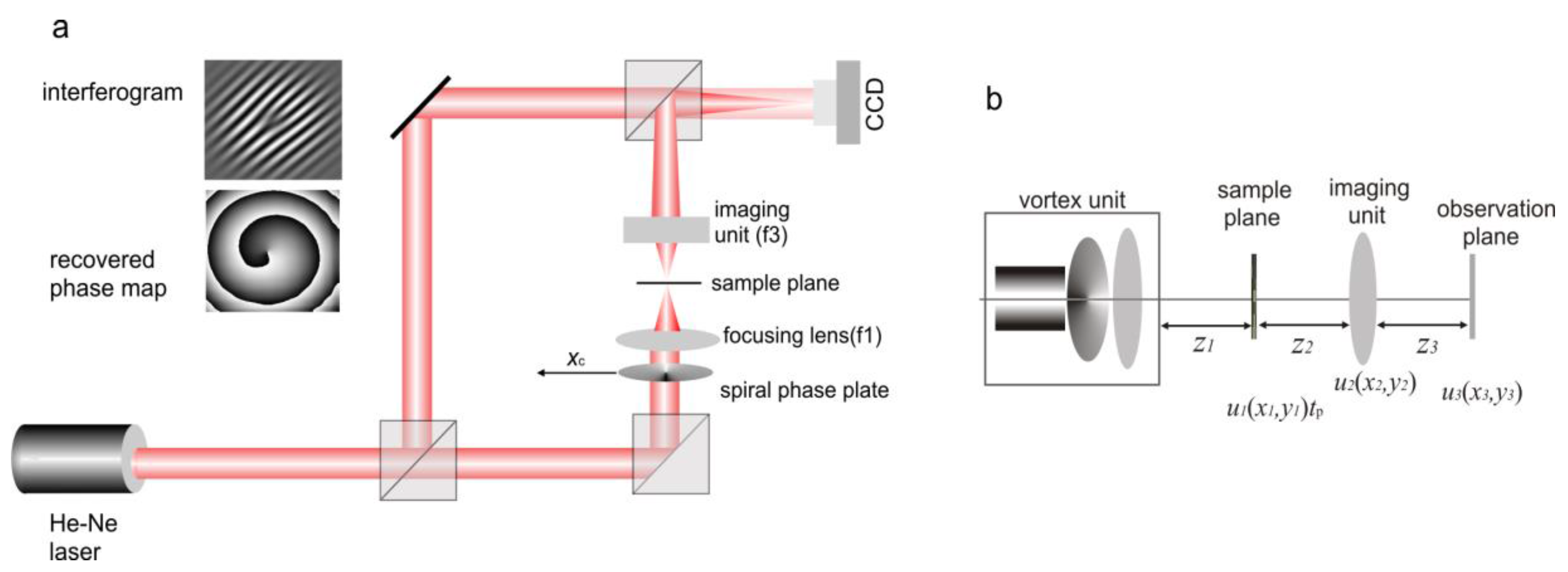
25]. The schematic view of our system is presented in Figure 1: the conventional Gaussian beam passes through the spiral phase plate and is focused on the sample plane, where it interacts with the investigated object. The sample plane is imaged into the CCD camera. The interferometer’s reference arm enables detection of the interference fringes, from which the internal structure of the object beam can be recovered. The important part of the OVSM metrology procedures is the internal scanning method (ISM). ISM [26,27] is realized by moving the vortex lens [28,29] perpendicularly to the direction of the incident laser beam. In this method, the sample needs to be scanned just by an optical vortex, while the entire focused beam stays in one place. The intriguing properties of the ISM were discussed in some papers [30,31].
To develop procedures for the object topography reconstruction from the images recorded with the OVSM, a good theoretical understanding of the instrument is necessary. Previous papers [32,33] presented an analytical description of the OVSM in the scalar Fresnel approximation. The calculations were divided into three parts (Figure 1b). In the first part, the laser beam propagation through the vortex unit to the sample plane was calculated [32]. The calculations were difficult due to the off-axis position of the vortex lens. The derived formulas (Equation (1)) were in good agreement with the experimental results. In particular, the observed vortex trajectory rotation when the observation plane moves away from the vortex unit was in accordance with the calculations. This rotation allows an experimental determination of the optimal sample plane’s position, which is called critical plane. In the second part, the vortex beam propagation through the entire OVSM system, with no sample, was described [33]. It was shown there that a vortex beam propagation across any number of lenses (in paraxial approximation) can be described in terms of a function G (Equation (2)) with coefficients As, Bs;x, Bs;y, Cs, and Ω, that can be calculated from the parameters of the set-up (see [33] for details). Hence, the complex amplitude at the plane—zs can be expressed by:
u s ( x s , y s ) = Ω s e i k 2 z s ( x s 2 + y s 2 ) G ( A s , B s ; x , B s ; y , C s ) ,
where
G ( A s , B s ; x , B s ; y , C s ) = π e C s 2 A s { π n = 0 1 n ! ( 2 A s ) 2 n + 1 j = 0 2 n + 1 ( 2 n + 1 j ) B s ; x j B s ; y 2 n + 1 j l = 0 m J m + j l , 2 n + 2 j + l ; m o d d n = 0 1 ( 2 n + 1 ) ! ! ( 2 A s ) 2 n + 2 j = 0 2 n + 2 ( 2 n + 2 j ) B s ; x j B s ; y 2 n + 2 j l = 0 m J m + j l , 2 n + 2 j + l ; m e v e n
Here, m is the topological charge of the optical vortex. Formula (1) can be used for any integer m; however, in the case of the OVSM, we limit it to the simplest case m = 1. Index s indicates the step of our calculations. The case of s = 1 determines the sample plane; for s = 2, we are at the imaging unit plane; s = 3 determines the observation plane located by the CCD camera (Figure 1b). Ωs is a complex constant. The derived formulas for the complex amplitude at the OVSM observation plane z3 are:
u 3 ( x 3 , y 3 ) = 4 π 2 k 2 γ 2 γ 3 e i k 2 z 3 ( x 3 2 + y 3 2 ) G ( A 3 , B 3 ; x , B 3 ; y , C 3 ) ,
A 3 = α i k ( β + 1 2 z 1 2 γ 2 + 1 2 z 1 2 z 2 2 γ 2 2 γ 3 )
B 3 ; x = 2 x c ( α + i k ( β + 1 2 z 1 2 γ 2 + 1 2 z 1 2 z 2 2 γ 2 2 γ 3 ) ) i k 2 z 1 z 2 z 3 γ 2 γ 3 x 3 , B 3 ; y = i k z 1 z 2 z 3 γ 2 γ 3 y 2
C 3 = x c 2 ( α + i k ( β + 1 2 z 1 2 γ 2 + 1 2 z 1 2 z 2 2 γ 2 2 γ 3 ) ) i k x c 2 γ 3 ( x 3 2 z 3 2 + y 3 2 z 3 2 2 x 3 x c z 1 z 2 z 3 γ 2 )
γ 2 = 1 z 1 + 1 z 2 , γ 3 = 1 z 2 + 1 z 3 1 f 3 1 z 2 2 γ 2
α = 1 w 2 , β = 1 2 ( 1 R + 1 f 1 1 z 0 ) , w 2 = w 0 2 ( 1 + ( λ z 0 π w 0 2 ) 2 ) ; R = z 0 ( 1 + ( π w 0 2 λ z 0 ) 2 )
where k is a wavenumber, z1, z2, and z3 are distances shown in Figure 1b, f1 is the focal length of the focusing lens in the vortex unit (Figure 1b), f3 is the focal length of the imaging unit, xc is a vortex lens shift (Figure 1a), w0 is the beam waist, and z0 is the distance between the Gaussian beam waist plane and the vortex unit.
In [33], the formulas for the vortex trajectory at the observation plane z3 were also given, and the position of the critical plane was found (where the vortex trajectory is perpendicular to the phase plate shift). It was shown that between the sample plane and the observation plane, the trajectory behaves like a standard object in classical imaging: the trajectory angle is preserved and magnified according to classical formula.
The third part of our calculations, which is the subject of this paper, includes a basic phase object located at the sample plane (Figure 1b). This paper presents the results and finishes the whole series. The next section describes the theory. Section 3 provides a brief discussion of the analytical calculations; Section 4 presents the experimental results; Section 5 concludes the paper.

2. Basic Phase Sample

The previous paragraph showed how the laser beam propagation through the OVSM system (Figure 1b) can be calculated. Since the phase and amplitude of the beam can be directly computed, the reference arm of the OVSM (Figure 1a) was neglected in the calculations. In the next step, the object is put in the sample plane, which coincides with the critical plane (or is very close to it). The critical plane is a plane where the vortex trajectory is perpendicular to the vortex lens shift [27,30,31]. The vortex point (i.e., the point where the phase is singular) is most sensitive at this location. The object is a glass plate with a small rectangular phase groove or pillar. Its center is at position xs, ys, and its size is sx and sy. The object introduces an additional phase shift ±ψ. This small object is expected to have little impact on the total diffraction spot at the observation plane. However, there is an optical vortex in the middle of the beam. The core of the optical vortex is almost dark, and its phase changes rapidly rendering this insignificant influence detectable. The focused vortex beam illuminating the sample can be represented in a general form:
u 1 ( x 1 , y 1 ) = a ( x 1 , y 1 ) e i φ ( x 1 , y 1 ) .
The rectangle phase object transmittance function is
t p ( x 1 , y 1 ) = e i Π ( x 1 x s s x , y 1 δ y s s y ) ψ .
where Π is a rectangular function.
Just behind the sample plane, we have:
u 1 ( x 1 , y 1 ) = a ( x 1 , y 1 ) e i Π ( x 1 x s s x , y 1 y s s y ) ψ + i φ ( x 1 , y 1 )
The above exponential function can be expanded into a power series against the phase shift ψ:
a 1 e i Π ψ + i φ = a 1 e i φ + a 1 e i φ Π ( i ψ 1 2 ψ 2 i 6 ψ 3 + 1 24 ψ 4 + ) = a 1 e i φ u v b + a 1 e i φ Π ( e i ψ 1 ) u o b
which means that behind the object plane, the beam can be written as a sum of the free propagating vortex beam uvb and the object beam uob. An object beam is a vortex beam multiplied by a rectangular function and a constant phase term. The vortex beam uvb was already calculated and given in Formula (3) with the proper coefficients (4)–(6) (see [33]). Now, the object beam uob needs to be calculated. The object is assumed to be so small that the phase and amplitude variations inside the rectangle can be neglected. Hence:
a ( x 1 , y 1 ) e i φ ( x 1 , y 1 ) Π ( x 1 x s s x , y 1 y s s y ) ( e i ψ 1 ) a ( x s , y s ) e i φ ( x s , y s ) Π ( x 1 x s s x , y 1 y s s y ) ( e i ψ 1 )
where xs and ys are coordinates of the rectangle center. With the Fresnel diffraction integral, the complex amplitude distribution of the object term at imaging unit plane (Figure 1b) can be calculated
u o b ( x 2 , y 2 ) = 1 i λ z 2 e i k 2 z 2 ( x 2 2 + y 2 2 ) a ( x s , y s ) e i φ ( x s , y s ) ( e i ψ 1 ) R 2 Π ( x 1 x s s x , y 1 y s s y ) e i k 2 z 2 ( x 1 2 + y 1 2 ) e i k z 2 ( x 1 x 2 + y 1 y 2 ) d x 1 d y 1
By applying the substitution
x 1 = x s + x ; y 1 = y s + y
the coordinate system is moved to the rectangle center, and the integral takes the form
u o b ( x 2 , y 2 ) = Ω R 2 Π ( x s x , y s y ) e i k 2 z 2 ( x 2 + y 2 ) e i k z 2 [ x ( x 2 x s ) + y ( y 2 y s ) ] d x d y
Ω = 1 i λ z 2 e i k 2 z 2 ( x 2 2 + y 2 2 ) e i k 2 z 2 ( x s 2 + y s 2 ) e i k z 2 ( x s x 2 + y s y 2 ) a ( x s , y s ) e i φ ( x s , y s ) ( e i ψ 1 )
Since the phase object is small compared to the distance z2, the phase variation of the quadrature term is also small; thus, the whole exponential term can be considered to be constant:
u o b ( x 2 , y 2 ) = Ω R 2 Π ( x s x , y s y ) e i k z 2 [ x ( x 2 x s ) + y ( y 2 y s ) ] d x d y
The integral has a solution:
R 2 Π ( x s x , y s y ) e i k z 2 [ x ( x 2 x s ) + y ( y 2 y s ) ] d x d y = s x s y sin c ( k s x 2 z 2 ( x 2 x s ) ) sin c ( k s y 2 z 2 ( y 2 x s ) )
Finally, we have:
u o b ( x 2 , y 2 ) = s x s y Ω sin c ( k s x 2 z 2 ( x 2 x s ) ) sin c ( k s y 2 z 2 ( y 2 y s ) )
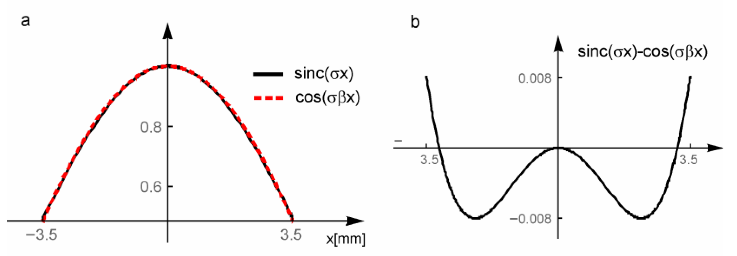
This formula describes the complex amplitude distribution of the phase object term at the imaging unit plane. In the final step, its image at the observation plane must be calculated. The sinc function results in long expressions; therefore, it can be replaced by the cosine function, properly adjusted by the β factor, as shown in Figure 2. This is possible as the rectangle is small enough for its image to be widely spread over the imaging unit aperture. As a result, only the central part of this image passes through the imaging unit. Then, the replacement formula takes the form:
sin c ( k s x 2 z 2 ( x 2 x s ) ) cos ( β k s x 2 z 2 ( x 2 x s ) ) ; sin c ( k s y 2 z 2 ( y 2 y s ) ) cos ( β k s y 2 z 2 ( y 2 y s ) )
and (20) takes the form
u o b ( x 2 , y 2 ) = s x s y Ω cos ( β k s x 2 z 2 ( x 2 x s ) ) cos ( β k s y 2 z 2 ( y 2 x s ) )
Expression (22) evaluates the complex amplitude of the beam part at the imaging unit plane (Figure 1b). Now, this solution needs to be multiplied by the lens transmittance function, and then the complex amplitude distribution at the observation plane is determined. The lens transmittance function is t L = exp { i k / 2 f 2 ( x 2 2 + y 2 2 ) } . Applying the Fresnel diffraction integral, we get:
u o b ( x 3 , y 3 ) = Ξ Σ cos ( β k s x 2 z 2 ( x 2 x s ) ) cos ( β k s y 2 z 2 ( y 2 y s ) ) e i k ( x 2 ( x s z 2 + x 3 z 3 ) + y 2 ( y s z 2 + y 3 z 3 ) ) e i k 2 ( x 2 2 + y 2 2 ) ( 1 z 2 + 1 z 3 1 f 2 ) d x 2 d y 2
Ξ = 1 i λ 2 z 2 z 3 s x s y a ( x s , y s ) e i φ ( x s , y s ) ( e i ψ 1 ) e i k 2 z 2 ( x s 2 + y s 2 ) e i k 2 z 3 ( x 3 2 + y 3 2 )
where ∑ is an aperture area. The first element of the imaging unit is the microscopic objective with a circular aperture with a diameter equal to 7 mm. Our main interest is the central part of the beam at the observation plane. In such a case, the circular aperture can be replaced by a rectangular one. At this stage of research, the results calculated for the rectangular area are valuable, and the final formulas are much simpler. With a square aperture, the following integrals must be computed:
int x = r r cos ( ξ s x ( x 2 x s ) ) e i χ x x 2 e i k 2 x 2 2 ( 1 z 2 + 1 z 3 1 f 2 ) d x 2
int y = r r cos ( ξ s y ( y 2 y s ) ) e i χ y x 2 e i k 2 y 2 2 ( 1 z 2 + 1 z 3 1 f 2 ) d y 2
ξ = β k 2 z 2 , χ x = k ( x s z 2 + x 3 z 3 ) , χ y = k ( y s z 2 + y 3 z 3 )
The solutions are:
int x = ( 1 ) 3 4 2 k β π 2 e i 1 2 ( 2 s x x s + ( s x ξ + χ x ) 2 k β ) [ e 2 i s x ξ χ x k β ( erfi ( ( 1 2 + i 2 ) ( k r β + s x ξ χ x ) k β ) + erfi ( ( 1 2 + i 2 ) ( k r β s x ξ + χ x ) k β ) ) + e 2 i s x ξ x s ( erfi ( ( 1 2 + i 2 ) ( k r β + s x ξ + χ x ) k β ) erfi ( ( 1 2 + i 2 ) ( k r β + s x ξ + χ x ) k β ) ) ]
int y = ( 1 ) 3 4 2 k β π 2 e i 1 2 ( 2 s y y s + ( s y ξ + χ y ) 2 k β ) [ e 2 i s y ξ χ y k β ( erfi ( ( 1 2 + i 2 ) ( k r β + s y ξ χ y ) k β ) + erfi ( ( 1 2 + i 2 ) ( k r β s y ξ + χ y ) k β ) ) + e 2 i s y ξ y s ( erfi ( ( 1 2 + i 2 ) ( k r β + s y ξ + χ y ) k β ) erfi ( ( 1 2 + i 2 ) ( k r β + s y ξ + χ y ) k β ) ) ]
where erfi is the error function [34]. Thus, the whole solution is:
u ( x 3 , y 3 ) = u v b ( x 3 , y 3 ) + u o b ( x 3 , y 3 )
u o b ( x 3 , y 3 ) = Ξ int x int y
u v b = 4 π 2 k 2 γ 2 γ 3 e i k 2 z 3 ( x 3 2 + y 3 2 ) G ( A 3 , B 3 x , B 3 y , C 3 )
For the conjugate planes, we have
1 z 2 + 1 z 3 1 f 3 = 0
and Expression (22) is reduced to:
int x = x s s x 2 x s + s x 2 cos ( ξ x x 2 ) e i x 2 χ x d x 2
int y = y s s y 2 y s + s y 2 cos ( ξ y y 2 ) e i x 2 χ y d y 2
The solutions are:
int x = 1 χ x 2 ξ x 2 [ e i 1 2 ( s x + 2 x s ) χ x i χ x cos ( ( s x 2 + x s ) ξ x ) + e i s x χ x ( i χ x cos ( ( s x 2 + x s ) ξ x ) + ξ x sin ( ( s x 2 + x s ) ξ x ) ) ξ x sin ( ( s x 2 + x s ) ξ x ) ]
int y = 1 χ y 2 ξ y 2 [ e i 1 2 ( s y + 2 y s ) χ y i χ y cos ( ( s y 2 + y s ) ξ y ) + e i s y χ y ( i χ y cos ( ( s y 2 + y s ) ξ y ) + ξ y sin ( ( s y 2 + y s ) ξ y ) ) ξ y sin ( ( s y 2 + y s ) ξ y ) ]
So far, the considered phase object has been small enough to assume the phase and amplitude inside its area to be constant (Equation (13)). This assumption is problematic at the areas of fast amplitude or phase changes. The first case occurs at the bright part of the vortex beam, the second one close to its center. The problem can be avoided by dividing the object into smaller parts. Each part inherits its own phase and amplitude values. The problem of extremely fast phase changes in the vicinity of a singular point (vortex point) is eliminated by the zero amplitude value. The transmittance function for the composed object becomes:
t p ( x 1 , y 1 ) = j = 1 N k = 1 M e i ψ Π ( x 1 x s ; j s x , y 1 δ y s ; k s y ) ,
where xs;j and ys;k are coordinates of the sub-rectangle at the j-th and k-th positions. Thus, the right side of Equation (13) can be rewritten:
a ( x 1 , y 1 ) e i φ ( x 1 , y 1 ) j = 1 N k = 1 M a ( x s ; j , y s ; k ) e i φ ( x s ; j , y s ; k ) Π ( x 1 x s ; j s x , y 1 y s ; k s y ) ( e i ψ 1 )
Here, all sub-rectangles are assumed to be both (1) the same size and (2) not overlapping; thus, (31) becomes
u o b ( x 3 , y 3 ) = j = 1 N k = 1 M Ξ j k int x ; j int y ; k
where intx;j and inty;k are values of intx and inty (36) and (37) is calculated for the sub-rectangle at the j-th row and k-th column. Ξ j k is the value for Ξ (24) for the rectangle at the j-th row and k-th column.
The derived formulas are complicated; however, some interesting conclusions concerning image creation by the OVSM can be drawn on the basis of these formulas. Also, they show a way for the future development of image reconstruction procedures. This will be discussed in the next section.

3. Numerical Examples

In this section, we briefly present the basic conclusions derived from our theory and its experimental verification. We start with a one micron phase square etched in a glass plate, introducing the phase shift ψ = −π into the incident laser beam. The glass plate with this square phase groove is positioned at the sample plane. The vortex lens shift is xc = 0. The phase square is decomposed into 8 × 8 sub-rectangles. The numerical examples were calculated using Formula (40). Figure 3 shows the amplitude and phase distribution of the vortex beam at the sample and observation planes of the OVSM optical system (Figure 1b).
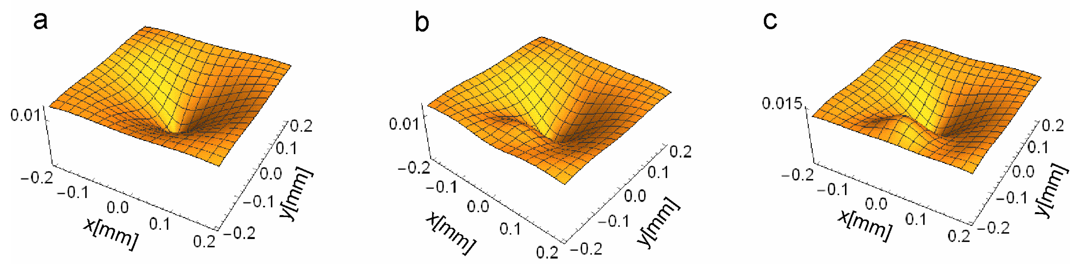
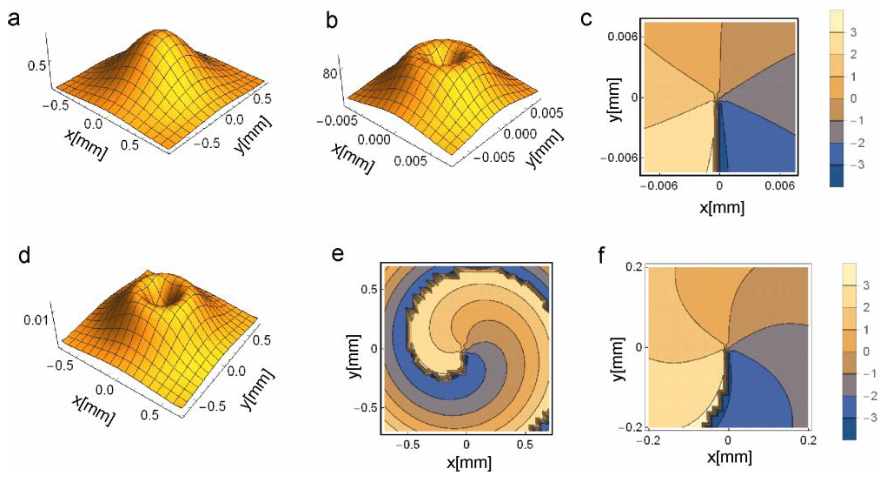
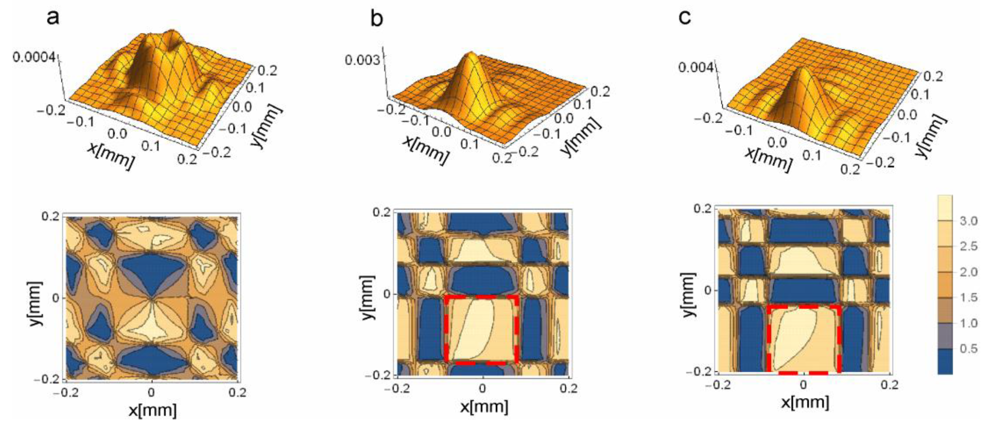
Figure 4 shows the amplitude and phase distribution at the observation plane of the object beam uob for three different y-positions of the square groove within the beam (the groove position is changed perpendicularly to the optical axis). When the phase square center is at the beam center (y = 0), the resulting amplitude at the observation plane is low, and the characteristic zero amplitude point is at the image center. The phase distribution reveals a characteristic vortex structure (column (a)).
Moving the sample (phase square) center off-axis results in a higher image amplitude, and the image center becomes free from optical vortex. The image has a higher amplitude because the phase square is illuminated by the ring part of the vortex beam. The phase maps (b and c) reconstruct the phase square. We can see a rectangle of almost constant phase (marked by a dashed red line), which moves when the object is moved. The image size results from both system magnification and diffraction. For the one micron-size rectangle and objective with NA = 0.4, the diffraction has a remarkable impact on the image and the image is about two times larger than the object.
Figure 5 shows the amplitude and phase distribution of the total beam uvb + uob for different positions of the square groove within the beam (the same as in Figure 4). In part b and c, the amplitude distribution of the vortex beam is modified by the object part in a visible way.

4. Experimental Results

To verify our theoretical calculations, the measurements were performed in the system shown schematically in Figure 1a. The He-Ne laser beam passed through the spiral phase plate and was focused by the microscope objective (×20, NA = 0.4) to the sample plane. The size of the vortex ring at the sample plane was 6.5 μm. The sample plane was observed by the CCD camera through the imaging unit (magnification 160×), which consisted of the microscopic objective (×20, NA = 0.4) and the additional lens of an effective focal length equal to 25 mm. The recorded interferograms were proceeded using carrier frequency techniques, as described in a previous paper [31]. In this way, the phase and amplitude distribution of the object beam was reconstructed. In the first step, we recorded the reference interferogram (without the object), which is the part 
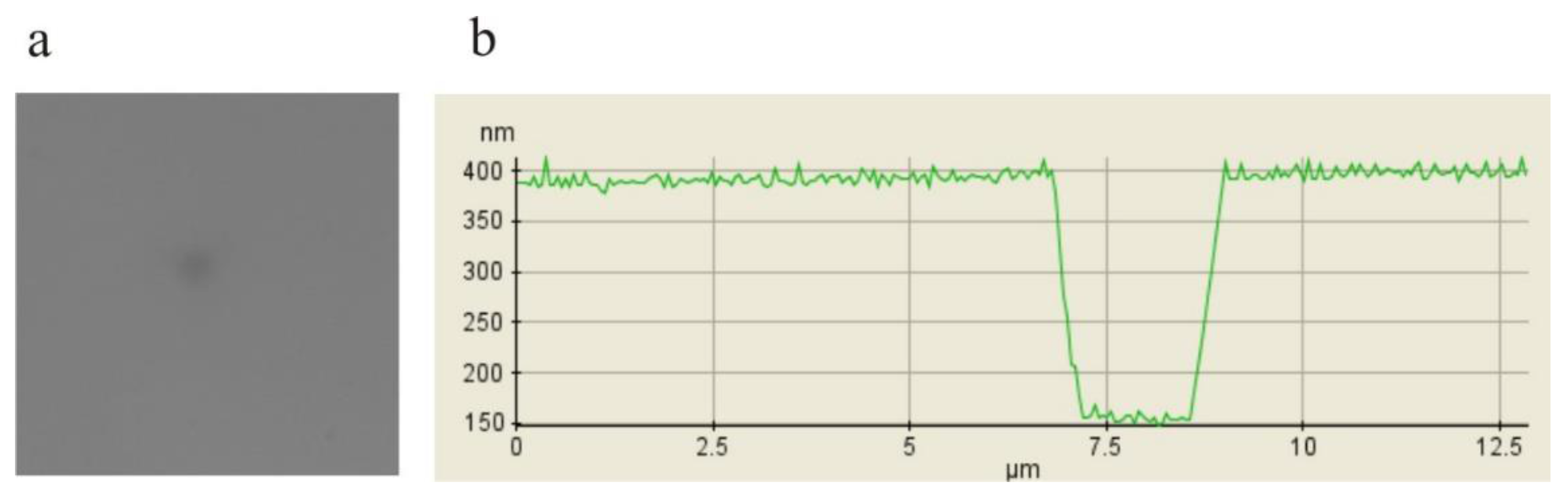
uvb in Formula (12). The phase and amplitude part of the reference beam were extracted. Next, the phase square 1 μm × 1 μm in size and 250 nm in depth was inserted into the sample plane. Figure 6a presents the white light image of this sample as seen by the CCD camera in the set-up presented in Figure 1. As this image is fine and of low contrast, the Atomic Force Microscopy profile is also shown in Figure 6b.
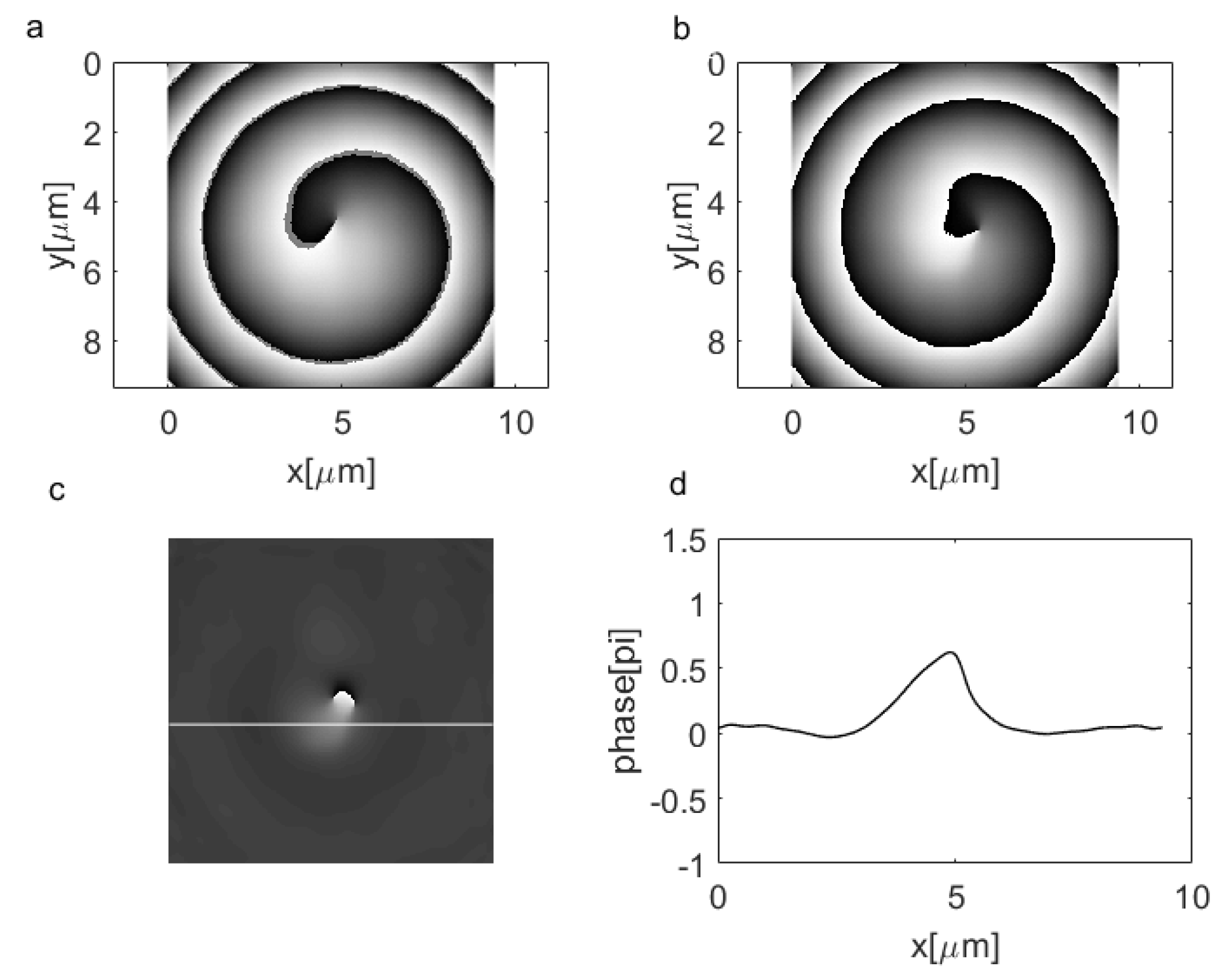
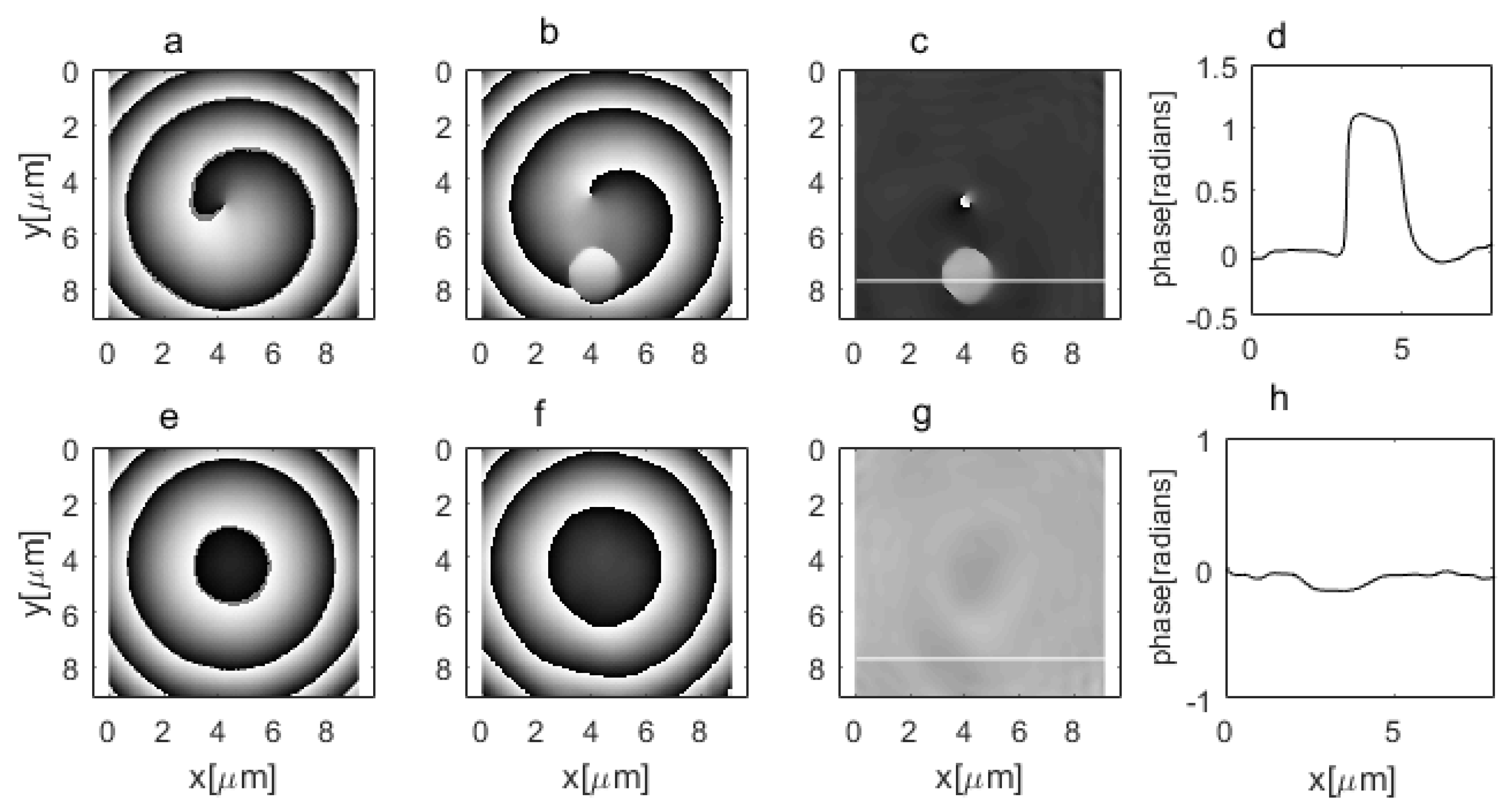
Figure 7 shows the result of the phase map reconstruction. The reference image was subtracted from the total image (Figure 7b), and the resulting complex amplitude was multiplied by the complex conjugate amplitude of the reference image (Figure 7c). Figure 7b shows that by using this procedure, an image of the sample was obtained. Figure 7d shows the profile of the image along the line shown in Figure 7c. The measured phase depth is almost 1.2 radians, as was expected. The width evaluated from the experimental conditions is 1.9 μm, which is larger due to the diffraction effects and consistent with the effect observed in Figure 4, where the diffraction spot representing the phase square image was doubled due to diffraction effects. Although the calculations were performed for the imaging unit magnification 80×, the numerical aperture was the same as in the experiments. So, we expect a blurring of the image due to diffraction by the same factor.
The one micron phase square is large enough to be reconstructed without breaking the classical resolution limit. However, here we tested our analytical model and the resulting reconstruction procedure. To do so, a sample with well-controlled geometry was necessary. Moreover, with an objective with NA = 0.4, a phase object 1 μm × 1 μm in size can hardly be seen (Figure 6a). We applied the same reconstruction procedure for the pure Gaussian beam. The vortex plate was removed, and the set-up was aligned for imaging with a non-vortex beam. Figure 7e–h show the results. Now, the reference beam was free from vortex. There was no trace of the sample after reference beam subtraction (Figure 7b), and it was hardly visible after multiplication by the conjugated reference beam (Figure 7c).
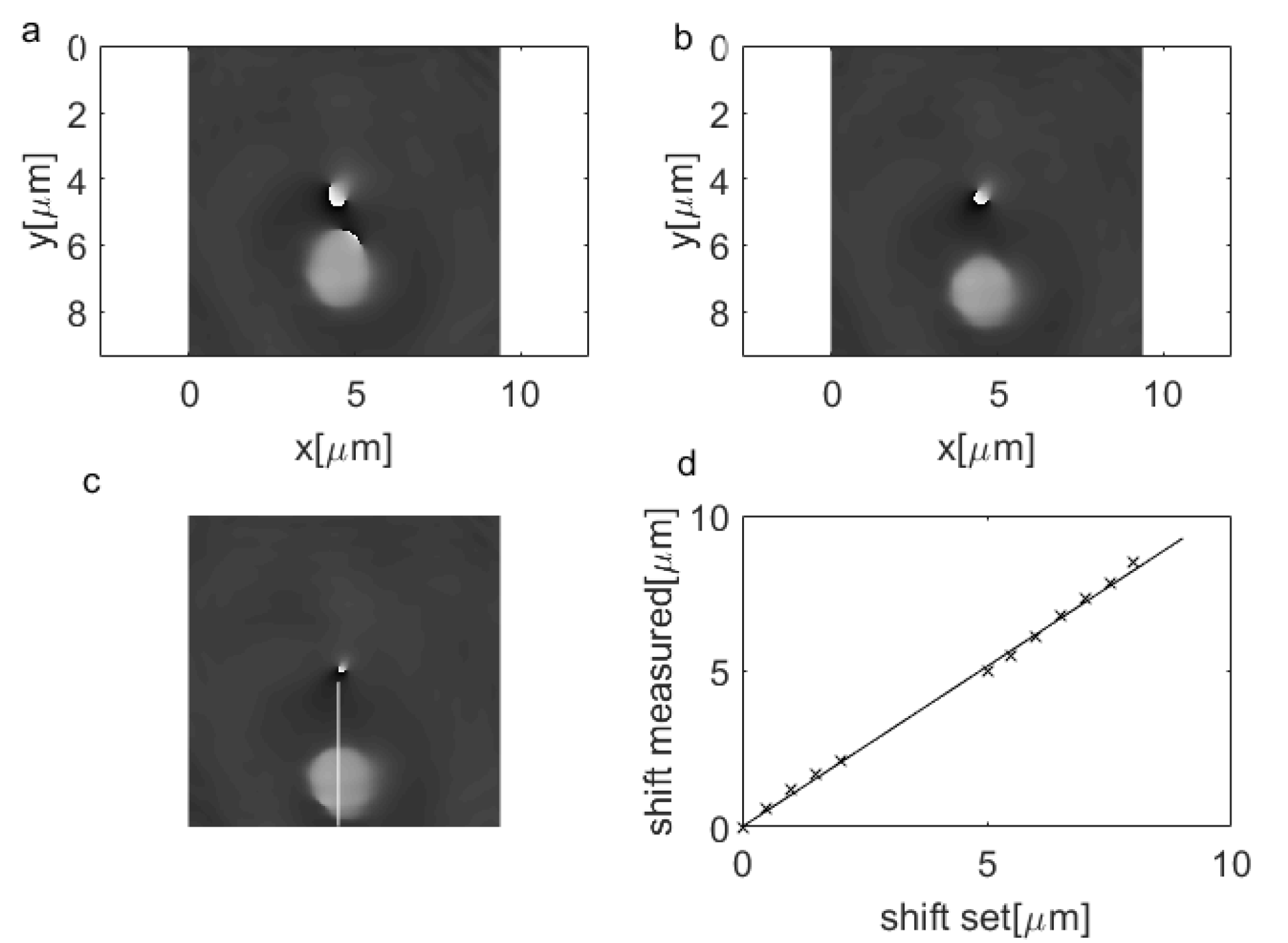
In the experiment, we also measured the position of the groove within the beam for different microscope table shifts (Figure 8a–c). The sample was moved with steps equal to 0.5 μm. We traced the position of the sample on the phase maps and compared it with the shift set by the microscope table driver. The results are shown in Figure 8d.
Figure 9 shows the phase square image when its center is close to the vortex beam center. The vortex beam center is dark, so the square is illuminated by almost no light. As a result, its image is very poor. The same can be seen in 
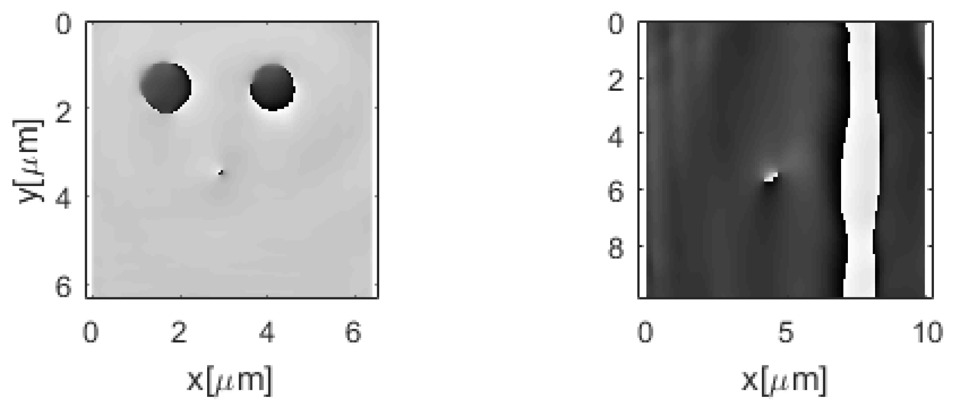
Figure 5a. Examples of the imaging of two other phase samples are shown in Figure 10.
These examples showed that vortex beam illumination opens the gate for high-resolution microscopic systems (such as OVSM). The presented analytical model of the OVSM was a starting point for developing a first procedure of object beam reconstruction. Images of the phase objects were obtained. The procedure is both simple and fast. The results obtained from the calculations based on the model are in good agreement with the experiment. However, there is certainly still a lot of room for developing more sophisticated and accurate reconstructing procedures.

5. Conclusions

For the first time, a theory for the scalar description of imaging using the OVSM was presented. This theory was tested experimentally and supported the general idea of imaging using OVSM. The focused vortex beam interacts with the object and transmits the corresponding information to the detection plane. The beam at the detection plane can be separated into a non-disturbed vortex part uvb and an object beam uob. The intensity of the non-disturbed part is spread out over the center, so the small disturbance introduced by the object can be detected at the image center. In some respects, the idea of the OVSM is similar to the vortex coronagraph project [35,36]. The vortex coronagraph uses the vortex lens as a special phase filter. The image of a centrally located star occupies the central part of the image. The telescope with the vortex lens spreads its light out of the image center. Thus, the off-axis planet can be observed in the central dark core of the vortex beam.
In our system, the image of the object was combined with the structure of the vortex beam. Nevertheless, the phase distribution of the object can be reconstructed, as shown in Figure 6. This is the simplest way of object reconstruction. Moreover, this model of the OVSM opens up new possibilities for the development of reconstruction procedures and for optical system optimization. This will be the subject of our next communication.

Acknowledgments

This work was supported by the Polish National Science Center (decision DEC-2013/11/B/ST7/01155).

Author Contributions

Agnieszka-Popiołek-Masajada conceived, designed, and performed the experiments and data analysis; Jan Masajada contributed analytical calculations, and Piotr Kurzynowski performed the experiments and data analysis.

Conflicts of Interest

The founding sponsors had no role in the design of the study; in the collection, analyses, or interpretation of data; in the writing of the manuscript, and in the decision to publish the results.

References

  1. Tychinsky, V.P.; Maslov, I.N.; Pankov, V.L.; Ublinsky, D.V. Computerized phase microscope for investigation of submicron structures. Opt. Commun. 1989, 74, 37–40. [Google Scholar] [CrossRef]
  2. Tychinsky, V.P.; Velzel, C.H. Super-Resolution in Microscopy. In Current Trends in Optics; Academic Press: Cambridge, MA, USA, 1994; Chapter 18. [Google Scholar]
  3. Totzeck, M.; Tiziani, H.J. Phase-singularities in 2D diffraction fields and interference microscopy. Opt. Commun. 1997, 138, 365–382. [Google Scholar] [CrossRef]
  4. Spektor, B.; Toker, G.; Shamir, J.; Friedman, M.; Brunfeld, A. High resolution surface feature evaluation using multiwavelength optical transforms. Proc. SPIE 2002, 4777, 345–351. [Google Scholar]
  5. Spektor, B.; Normatov, A.; Shamir, J. Singular beam microscopy. Appl. Opt. 2008, 47, A78–A87. [Google Scholar] [CrossRef] [PubMed]
  6. Spektor, B.; Normatov, A.; Shamir, J. Singular beam scanning microscopy: Preliminary experimental results. Opt. Eng. 2010, 49, 048001. [Google Scholar] [CrossRef]
  7. Fürhapter, S.; Jesacher, A.; Bernet, S.; Ritsch-Marte, M. Spiral phase contrast imaging in microscopy. Opt. Express 2005, 13, 689–694. [Google Scholar] [CrossRef] [PubMed]
  8. Jesacher, A.; Fürhapter, S.; Bernet, S.; Ritsch-Marte, M. Shadow effects in spiral phase contrast microscopy. Opt. Express 2005, 94, 233902. [Google Scholar] [CrossRef] [PubMed]
  9. Klar, T.; Engel, E.; Hell, S.W. Breaking Abbe’s diffraction resolution limit in fluorescence microscopy with stimulated emission depletion beams of various shapes. Phys. Rev. E 2001, 64, 066613. [Google Scholar] [CrossRef] [PubMed]
  10. Wang, W.; Yokozeki, T.; Ishijima, R.; Takeda, M.; Hanson, S.G. Optical vortex metrology based on the core structures of phase singularities in Laguerre-Gauss transform of a speckle pattern. Opt. Express 2006, 14, 10195–10206. [Google Scholar] [CrossRef] [PubMed]
  11. Wang, W.; Yokozeki, T.; Wada, R.A.; Miyamoto, Y.; Takeda, M.; Hanson, S.G. Optical vortex metrology for nanometric speckle displacement measurement. Opt. Express 2006, 14, 120–127. [Google Scholar] [CrossRef] [PubMed]
  12. Helseth, L.E. Smallest focal hole. Opt. Commun. 2006, 257, 1–8. [Google Scholar] [CrossRef]
  13. Masajada, J.; Leniec, M.; Jankowska, E.; Thienpont, H.; Ottevaere, H.; Gomez, V. Deep microstructure topography characterization with optical vortex interferometer. Opt. Express 2008, 16, 19179–19191. [Google Scholar] [CrossRef] [PubMed]
  14. Dennis, M.R.; Götte, J.B. Topological aberration of optical vortex beams: determining dielectric interfaces by optical singularity shifts. Phys. Rev. Lett. 2012, 109, 183903. [Google Scholar] [CrossRef] [PubMed]
  15. Tong, Z.; Korotkova, O. Beyond the classical Rayleigh limit with twisted light. Opt. Lett. 2012, 37, 2595–2597. [Google Scholar] [CrossRef] [PubMed]
  16. Masajada, J.; Leniec, M.; Drobczyński, S.; Thienpont, H.; Kress, B. Micro-step localization using double charge optical vortex interferometer. Opt. Express 2009, 17, 16144–16159. [Google Scholar] [CrossRef] [PubMed]
  17. Wojnowski, D.; Jankowska, E.; Masajada, J.; Suszek, J.; Augustyniak, I.; Popiołek-Masajada, A.; Ducin, I.; Kakarenko, K.; Sypek, M. Surface profilometry with binary axicon-vortex and lens-vortex optical elements. Opt. Lett. 2014, 39, 119–122. [Google Scholar] [CrossRef] [PubMed]
  18. Pascuci, M.; Tessier, G.; Emiliani, V.; Guillon, M. Superresolution imaging of optical vortices in a speckle pattern. Phys. Rev. Lett. 2016, 116, 093904. [Google Scholar] [CrossRef] [PubMed]
  19. Rogers, E.T.F.; Lindberg, J.; Roy, T.; Savo, S.; Chad, J.E.; Dennis, M.R.; Zheludev, N.I. A super-oscillatory lens optical microscope for subwavelength imaging. Nat. Mater. 2012, 11, 432–435. [Google Scholar] [CrossRef] [PubMed]
  20. Berry, M.V. A note on superoscillations associated with Bessel beams. J. Opt. 2013, 15, 044006. [Google Scholar] [CrossRef]
  21. Greenfield, E.; Schley, R.; Hurwitz, I.; Nemirovsky, J.; Makris, K.G.; Segev, M. Experimental generation of arbitrarily shaped diffractionless superoscillatory optical beams. Opt. Express. 2013, 21, 13425–13435. [Google Scholar] [CrossRef] [PubMed]
  22. Gustafsson, M.G. Surpassing the lateral resolution limit by a factor of two using structured illumination microscopy. J. Microsc. 2008, 198, 82–87. [Google Scholar] [CrossRef]
  23. Best, G.; Amberger, R.; Baddeley, D.; Dithmar, S.; Heintzmann, R.; Cremer, C. Structured illumination microscopy of autofluorescent aggregations in human tissue. Micron 2011, 42, 330–335. [Google Scholar] [CrossRef] [PubMed]
  24. Sapna, A.; Shroff, J.R.; Fienup, D.; Williams, D.R. OTF compensation in structured illumination superresolution images. Proc. SPIE 2008, 7094, 709402. [Google Scholar]
  25. Aurélie, J.; Rainer, H. Superresolution multidimensional imaging with structured illumination microscopy. Annu. Rev. Mater. Res. 2013, 43, 261–282. [Google Scholar]
  26. Masajada, J.; Leniec, M.; Augustyniak, I. Optical vortex scanning inside the Gaussian beam. J. Opt. 2011, 13, 03571. [Google Scholar] [CrossRef]
  27. Augustyniak, I.; Popiołek-Masajada, A.; Masajada, J.; Drobczyński, S. New scanning technique for the optical vortex microscope. Appl. Opt. 2012, 51, C117–C124. [Google Scholar] [CrossRef] [PubMed]
  28. Khonina, S.N.; Kotlyar, V.V.; Shinkaryev, M.V.; Soifer, V.A.; Uspleniev, G.V. The phase rotor filter. J. Mod. Opt. 1992, 39, 1147–1154. [Google Scholar] [CrossRef]
  29. Swartzlander, G.A., Jr. Achromatic optical vortex lens. Opt. Lett. 2006, 31, 2042–2044. [Google Scholar] [CrossRef] [PubMed]
  30. Popiołek-Masajada, A.; Sokolenko, B.; Augustyniak, I.; Masajada, J.; Kohoroshun, A.; Bacia, M. Optical vortex scanning in an aperture limited system. Opt. Lasers Eng. 2014, 55, 105–112. [Google Scholar] [CrossRef]
  31. Masajada, J.; Augustyniak, I.; Popiołek-Masajada, A. Optical vortex dynamics induced by vortex lens shift—optical system error analysis. J. Opt. 2013, 15, 044031. [Google Scholar] [CrossRef]
  32. Plociniczak, Ł.; Popiołek-Masajada, A.; Szatkowski, M.; Wojnowski, D. Transformation of the vortex beam in the optical vortex scanning microscope. Opt. Las. Technol. 2016, 81, 127–136. [Google Scholar] [CrossRef]
  33. Plociniczak, Ł.; Popiołek-Masajada, A.; Masajada, J.; Szatkowski, M. Analytical model of the optical vortex microscope. Appl. Opt. 2016, 55, B20–B27. [Google Scholar] [CrossRef] [PubMed]
  34. Weisstein, E. “Erfi”. From MathWorld—A Wolfram Web Resource. Available online: http://mathworld.wolfram.com/Erfi.html (accessed on 30 May 2017).
  35. Swartzlander, G.A., Jr. Peering into darknees with a vortex spatial filter. Opt. Lett. 2001, 26, 497–499. [Google Scholar] [CrossRef] [PubMed]
  36. Swartzlander, G.A., Jr. The optical vortex coronagraph. J. Opt. A 2001, 11, 094022. [Google Scholar] [CrossRef]
Figure 1. (a) Optical scheme of the Optical Vortex Scanning Microscope (OVSM); the exemplary interferogram and the recovered phase maps; (b) OVSM optical system as it is represented in the analytical model. Vortex and magnifying units are represented by two-dimensional transmittance functions (thin element approximation).
Photonics 04 00038 g001
Figure 2. (a) Plot of the functions sinc(σx) and cos(σβx), σ = k s x / 2 z 2 ; (b) plot of the difference between sinc(σx) and cos(σβx), β = 0.557. Within the aperture radius, the difference is acceptably small (below 1%).
Photonics 04 00038 g002
Figure 3. Phase and amplitude of the beam at various planes of the OVSM optical system. (a) The amplitude of the incident Gaussian beam. The beam waist is w0 = 0.4 mm, the distance between the beam waist and the vortex unit plane (Figure 1b) is z0 = 600 mm, and the wavelength is λ = 632.8 nm; (b) the amplitude of the focused beam at the sample plane; (c) the phase of the focused beam at the sample plane; the focusing lens focal length is f1 = 9 mm, and the sample plane is a critical plane, which is located at z1 = 8.95 mm from the vortex unit; (d) the amplitude of the vortex beam uvb at the observation plane; (e) the phase of the vortex beam at the observation plane; (f) the same as (e), but shown at a reduced area. The distance between the sample plane and the imaging unit plane is z2 = 9.11 mm, and between the imaging unit and the observation plane it is z3 = 729 mm.
Photonics 04 00038 g003
Figure 4. Amplitude (top) and phase (bottom) of the object beam vob at the observation plane for three different positions of the phase square center ys within the beam: ys = 0 (a); ys = 1 μm (b), and ys = 1.5 μm (c). The phase square size is 1 μm × 1 μm. The focal length of the magnifying lens is f3 = 9 mm, and its diameter is d = 7 mm. The distance between the sample plane and the magnifying lens is z2 = 9.11 m, and the distance between the magnifying lens and the observation plane is z3 = 729 mm (Figure 1b), so the system magnification is 80×. The red-dashed rectangle shows the phase image of the rectangle. The absolute value of the phase is plotted at the phase portraits. In this way, the image is not blurred by 2π phase jumps.
Photonics 04 00038 g004
Figure 5. The total beam uvb + uob amplitude for three positions of the phase square center ys: ys = 0 (a); ys = 1 μm (b); and ys = 1.5 μm (c). The parameters are as in Figure 4.
Photonics 04 00038 g005
Figure 6. (a) Image of our sample detected by the CCD camera in white light; (b) scan of the square profile taken with the Atomic Force Microscope. The sample was etched in a polymer with refractive index n = 1.49.
Photonics 04 00038 g006
Figure 7. Recovering the image of the 1μm × 1μm-phase step with the OVSM: (a) Phase map of the image captured with the OVSM. The spiral phase distribution is characteristic of the vortex beam. (b) The phase map of the beam after subtracting the reference image. The image of the phase rectangle is readily seen. (c) To extract this image from the spiral background, the image from part (b) is multiplied by the conjugated reference image. (d) Phase profile taken along the line shown in part (c). The figures are rescaled by system magnification (160×). (eh) Same as above in the case where the vortex was removed from the beam; the trace of the sample is not visible.
Photonics 04 00038 g007
Figure 8. (ac) The recovered phase maps for different positions of the phase square within the beam; (d) the shift measured with OVSM. The solid line shows the position determined from the microscope table shift, and the crosses show the measured values (R = 0.999).
Photonics 04 00038 g008
Figure 9. Imaging of the 1 μm × 1 μm phase step with the vortex beam. The phase square center is at the vortex center: (a) The sum of the reference and object phase map; (b) the total image phase map after subtracting the reference image; the image of the phase rectangle is not seen; (c) to extract this image from the spiral background, the image from part (b) is multiplied by the conjugated reference image; (d) the phase profile taken along the line shown in part (c).
Photonics 04 00038 g009
Figure 10. Examples of the recovered phase maps of two more samples observed using the OVSM: two 1 μm × 1 μm phase squares separated by a distance of 2 μm (left), and phase groove of a width of 0.5 μm (right).
Photonics 04 00038 g010

