Article

Tightly Coupled LiDAR-IMU Positioning System Based on Semiconductor Optoelectronic LiDAR Sensing with Prior Map Constraints and Robust Relocalization Mechanism

1
College of Electronics and Information Science, Fujian Jiangxia University, Fuzhou 350108, China
2
Zhongshan Institute, Changchun University of Science and Technology, Zhongshan 528400, China
*
Author to whom correspondence should be addressed.
These authors contributed equally to this work.
Photonics 2026, 13(7), 629; https://doi.org/10.3390/photonics13070629
Submission received: 27 May 2026 / Revised: 17 June 2026 / Accepted: 22 June 2026 / Published: 29 June 2026

Abstract

Accurate and robust localization based on semiconductor optoelectronic LiDAR sensing is a fundamental prerequisite for autonomous navigation of mobile robots in complex scenarios. Traditional positioning methods based on semiconductor optoelectronic LiDAR sensors suffer from cumulative drift during long-term operation, while prior map-based positioning techniques often lack adaptability to dynamic environments. To address these challenges, this paper proposes a high-performance LiDAR-IMU tightly coupled positioning system integrating prior map constraints, LIO optimization, and an adaptive failure detection-relocalization mechanism. A high-precision global map constructed by LIO-SAM serves as the prior constraint to ensure global consistency of pose estimation, while the tightly coupled LIO framework maintains high accuracy and low latency in high-dynamic scenarios. The proposed dual-index failure detection strategy identifies localization anomalies in real time, and a Bag-of-Words (BoW)-based relocalization module rapidly restores precise positioning. Extensive simulations on MARSIM and physical experiments in structured, semi-structured, and feature-sparse environments demonstrate that the proposed system outperforms state-of-the-art (SOTA) methods including LIO-SAM, Ada-LIO, and Map-ICP. Specifically, the system achieves an Absolute Trajectory Error (ATE) root mean square (RMSE) of ≤0.06 m in physical experiments, a cumulative drift of ≤0.1 m per 100 m, and a relocalization success rate of ≥90% in feature-sparse scenes. These results validate the system’s superiority in accuracy, robustness, and real-time performance, providing a reliable signal-processing solution for semiconductor optoelectronic LiDAR-based sensing systems in complex practical applications.

1. Introduction

Semiconductor optoelectronic LiDAR sensors are core optoelectronic devices for environmental perception of mobile robots, whose signal processing and positioning algorithms directly determine device application performance. Autonomous localization technology is the core enabler for mobile robots to perform tasks such as inspection, navigation, and autonomous charging in unstructured environments [1]. According to the dependence on prior environmental information, localization methods are categorized into map-free localization and prior map-based localization [2]. Map-free localization, typically implemented via Simultaneous Localization and Mapping (SLAM), achieves real-time navigation by incrementally constructing maps while estimating poses [3]. Graph-based SLAM methods, as representative map-free techniques, offer high-precision trajectory and map estimation with excellent consistency and robustness [4]. However, the computational complexity of loop closure detection and global graph optimization results in a map update frequency below 1 Hz, which fails to meet the real-time requirements of high-dynamic mobile robot applications [5].
In contrast, prior map-based localization methods achieve fast and high-precision pose estimation by matching sensor data with pre-constructed high-precision maps, significantly reducing computational overhead and improving real-time performance [6]. Mobile robot localization can be further divided into local positioning and global positioning [7]. Local positioning assumes a known initial pose and updates incrementally using sensor data, while global positioning determines the robot’s pose in the global coordinate system without prior pose information, which also involves relocalization to recover positioning after drift or loss [8]. The reliability of relocalization directly affects the safety and autonomy of robots in long-term missions [9].
Existing global positioning methods for mobile robots include external marker-based (GPS, WiFi, and UWB), visual scene recognition-based, neural network-based, map matching-based, and Monte Carlo Localization (MCL) methods [10]. External marker-based methods provide global poses but are environment-dependent: GPS is ineffective indoors, while WiFi/UWB require additional infrastructure, leading to high deployment costs [11]. Visual-based methods utilize cameras or LiDAR to identify environmental features with high precision but are susceptible to illumination changes and occlusions [12]. Neural network-based methods exhibit strong adaptability but rely on large-scale labeled training data [13]. Map matching-based methods depend on high-precision maps and are suitable for scenarios with minimal environmental changes [14]. MCL methods achieve positioning based on probability distributions with good adaptability but suffer from high computational complexity [15].
Local positioning technologies include odometry, inertial navigation (IMU), LiDAR odometry, visual odometry (VO), and multi-sensor fusion [16]. Odometry- and IMU-based methods are prone to cumulative errors and long-term drift [17]. LiDAR and VO methods estimate poses via feature matching but encounter significant errors in textureless or dynamic scenes [18]. To enhance system robustness, multi-sensor fusion has become a research focus in recent years, integrating IMU, LiDAR, and cameras to complement each other’s advantages [19].
Despite these advancements, existing methods still face critical challenges: (1) LIO-based methods lack global constraints, leading to cumulative drift in long-term operation; (2) prior map-based methods are unstable in dynamic or feature-sparse environments due to unreliable feature matching; (3) most systems lack efficient failure detection and relocalization mechanisms, resulting in poor adaptability to complex scenarios [20]. The semiconductor optoelectronic LiDAR sensor used in this work is a solid-state or hybrid solid-state ranging device based on direct time-of-flight (dToF) or amplitude-modulated continuous-wave (AMCW) measurement principles, realizing three-dimensional environmental perception through a semiconductor laser emitter (wavelength typically 905 nm or 1550 nm) combined with an avalanche photodiode (APD) or single-photon avalanche diode (SPAD) receiver array. Compared with traditional rotating mechanical LiDAR, this type of sensor exhibits a smaller form factor, lower power consumption, and higher integration, but also presents distinct signal-noise characteristics: (1) single-photon detection sensitivity leads to shot-noise-dominated range measurement with standard deviation typically in the range 0.02 0.05 m under normal ambient light conditions; (2) multi-path interference and glass-surface specular reflection can generate ghost returns, requiring robust outlier filtering at the pre-processing stage; (3) the non-uniform angular resolution across the field of view (denser near the center, sparser at edges) affects feature extraction density and must be accounted for in adaptive threshold design. The RS-Helios-16P device employed in this study operates at 905 nm, with a ranging accuracy of ± 2 cm ( 1 σ ) and a range noise standard deviation of σ r = 0.02 m , which directly governs the residual weighting strategy for LiDAR measurement residuals.
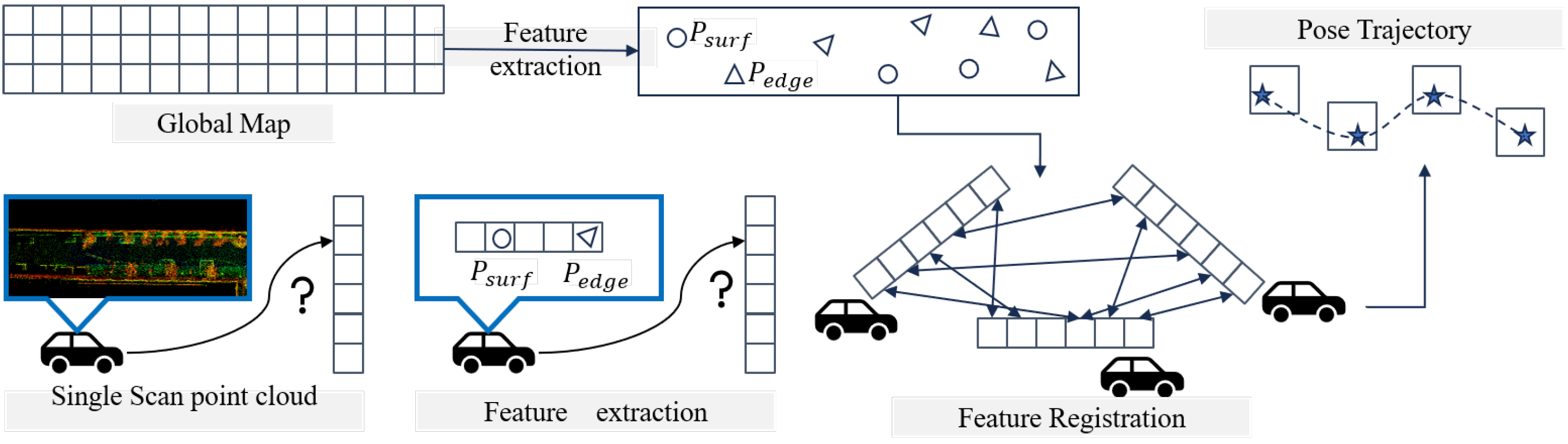
To address these issues and optimize the perception performance of semiconductor optoelectronic LiDAR devices, this paper proposes a high-robustness LiDAR-IMU positioning system integrating prior map constraints and LIO optimization, whose overall pipeline is illustrated in Figure 1. The main contributions of this work are threefold:
(1)
A prior map constraint framework is proposed, where a high-precision global map constructed by LIO-SAM is utilized to introduce map optimization terms. By precisely matching edge and planar features, cumulative drift during long-term operation is effectively suppressed, and the global consistency of pose estimation is improved.
(2)
A LiDAR-IMU tightly coupled optimization strategy is designed based on a factor graph framework. IMU pre-integration and LiDAR feature matching residuals are jointly optimized, ensuring high-precision and low-latency pose estimation even in high-dynamic environments.
(3)
An adaptive failure detection and relocalization mechanism is developed. A dual-index anomaly detection strategy (residual monitoring + pose jump detection) identifies localization failures in real time, and a BoW-based global matching method combined with RANSAC geometric verification achieves fast and accurate relocalization, significantly enhancing the system’s robustness in complex scenarios.

2. Related Work

2.1. LiDAR-IMU Tightly Coupled Localization

LiDAR-IMU tightly coupled localization has gained extensive attention due to its complementary advantages in high-frequency (IMU) and high-precision (LiDAR) applications. Early works such as LOAM [6] and LeGO-LOAM [21] laid the foundation for LiDAR odometry by extracting edge and planar features for pose estimation. LIO-SAM [22] further integrated IMU pre-integration into a factor graph optimization framework, achieving high-precision and real-time localization. However, these methods lack prior map constraints and suffer from cumulative drift in long-term operation.
To address state estimation degeneracy in low-texture environments such as long corridors and open squares, GIF-LIO [23] proposed a geometry-intensity fused LiDAR–inertial odometry framework with degeneracy-constrained state estimation. It constructs redundancy-aware geometric measurement constraints and fuses complementary intensity information to update system states only along high-information directions, suppressing drift in degenerate scenarios. Experimental validation on multiple public datasets showed that the method reduces trajectory RMSE by 4.2–8.5% in typical degenerate scenes compared with baseline LIO methods. Nevertheless, GIF-LIO does not incorporate prior map constraints, leading to unavoidable cumulative drift in long-term missions, and lacks a dedicated relocalization mechanism for positioning recovery.

2.2. Prior Map-Constrained Localization

VE-LIOM [24] proposed an efficient LiDAR-inertial odometry and mapping framework based on sparse factor graph optimization, integrating local submap maintenance and adaptive keyframe selection to reduce computational overhead in large-scale scenarios. An information-theoretic adaptive relocalization method InfoLa-SLAM [25] was developed to screen keyframes by environmental information richness and assist relocalization via landmark matching, reducing redundant computations and improving stability in dynamic environments. However, these methods fail to deeply fuse prior map constraints with LiDAR-IMU tight coupling, resulting in insufficient balance between global consistency and local dynamic responsiveness.
LIO-Fusion [26] introduced a reinforced LiDAR-inertial odometry framework with relocalization and multi-sensor fusion capabilities, reducing cumulative errors via prior-map matching and factor graph optimization. A coarse-to-fine registration strategy combining global candidate retrieval and local ICP optimization is adopted for relocalization, ensuring accurate matching with prior maps even in changing environments. However, the global retrieval-based relocalization leads to high computational overhead, and the lack of deep integration with tight-coupled LIO backend results in limited real-time performance in high-dynamic scenarios.

2.3. Relocalization for LiDAR-IMU Systems

LCR-Net [27] proposed a unified loop closing and relocalization framework with a multi-head feature extraction structure and pose-aware attention mechanism, enhancing the discriminability of LiDAR scan descriptors and achieving superior loop closure detection and relocalization accuracy on the KITTI dataset compared with traditional handcrafted methods. However, deep learning-based methods require large-scale training data and high computational resources, limiting their deployment on resource-constrained mobile robot platforms.
Transformer-based point cloud matching methods represented by RegiFormer [28] leverage local-to-global contextual attention to enhance the accuracy of LiDAR point cloud registration under low overlap, while end-to-end self-supervised LiDAR-inertial odometry systems [29] achieve high-precision pose estimation without manual pose labels by exploiting geometric consistency constraints. Nevertheless, these methods face challenges in engineering deployment and lack flexible anomaly handling mechanisms, leading to poor adaptability to rapidly changing environments.

2.4. Multi-Source Fusion Localization with Heterogeneous Sensors

Recent advances in multi-source fusion localization have demonstrated that combining heterogeneous sensing modalities within a tightly coupled framework significantly improves robustness in GNSS-denied or feature-degraded environments. Wang et al. [30] proposed a UWB/LiDAR tightly coupled positioning algorithm based on an improved sparrow search algorithm (ISSA)-optimized particle filter, embedding UWB range observations as absolute position anchors into a particle-weight update mechanism to suppress long-term LiDAR-SLAM drift; experiments in indoor environments demonstrated centimeter-level accuracy even under severe non-line-of-sight (NLOS) conditions. In contrast to the proposed system, which relies solely on a prior LiDAR map for global constraint without real-time UWB anchors, their approach requires infrastructure deployment but achieves stronger absolute positioning guarantees in known environments. Cai et al. [31] proposed a GPS-aided stereo inertial navigation localization algorithm for outdoor scenarios, fusing RTK-GPS absolute pose observations with stereo visual-inertial odometry via a tightly coupled factor graph; adaptive outlier rejection is applied to GPS measurements under multipath conditions, yielding sub-decimeter accuracy on long outdoor routes. Compared with their system, the proposed method replaces GPS with a pre-built LiDAR map as the global constraint source, making it applicable to both indoor and GPS-denied outdoor environments but placing a higher demand on prior map quality. These comparisons highlight that the tightly coupled fusion paradigm is consistently beneficial across different sensor configurations, and that the choice of global constraint (UWB anchors, GPS, or prior map) should be driven by deployment constraints, which is precisely the motivation for the prior-map-based design adopted in this paper.
In summary, existing methods have limitations in degeneracy robustness, relocalization efficiency, and constraint fusion depth. This paper addresses these gaps by: (1) deeply integrating prior map constraints with LiDAR-IMU tight coupling within a factor graph framework to balance global consistency and local dynamic performance; (2) designing a quantifiable anomaly detection index and efficient relocalization strategy to achieve a trade-off between real-time performance and recovery precision; and (3) specifying key parameters for feature extraction, registration, and constraint fusion to ensure engineering reproducibility. These innovations enable the proposed system to meet the requirements of high-precision, robust, and real-time localization for mobile robots in complex practical scenarios.

3. Methodology

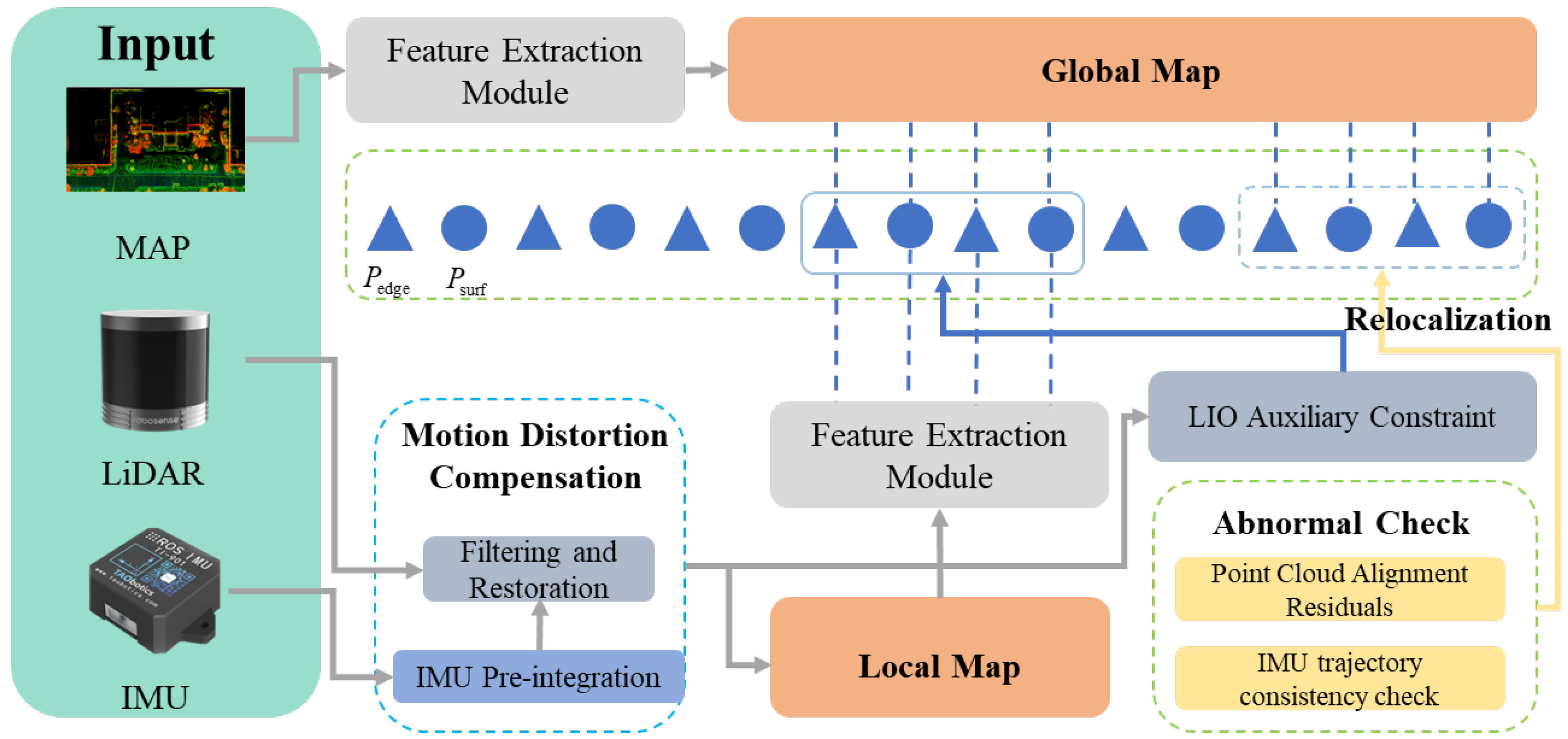
The framework of the proposed LiDAR-IMU tightly coupled positioning system is illustrated in Figure 2, consisting of four core modules: data preprocessing, prior map constraint, LIO tight coupling optimization, and failure detection & relocalization. This framework acts as an efficient real-time signal processing and pose estimation system for semiconductor optoelectronic LiDAR sensors. The data preprocessing module performs IMU pre-integration and LiDAR point cloud motion distortion correction. The prior map constraint module extracts features from real-time point clouds and matches them with the pre-constructed high-precision map to provide global pose constraints. The LIO tight coupling optimization module fuses IMU pre-integration residuals, LiDAR feature matching residuals, and odometry auxiliary constraints within a factor graph framework to estimate optimal poses. The failure detection & relocalization module identifies positioning anomalies in real time and triggers relocalization to restore precise positioning, ensuring long-term operational stability.

3.1. Data Preprocessing

3.1.1. IMU Pre-Integration

IMU provides high-frequency attitude and motion information, compensating for the low sampling rate and transient occlusions of LiDAR. Direct integration of raw IMU data into nonlinear optimization increases computational complexity, so IMU pre-integration is adopted to extract key state increments and construct inertial residuals between adjacent keyframes.
The system state vector is defined as X = [ p , v , R , b a , b g ] T , where p R 3 , v R 3 , and R S O ( 3 ) denote the position, velocity, and attitude rotation matrix in the world frame, respectively; b a R 3 and b g R 3 represent the biases of the accelerometer and gyroscope. The IMU measurement model is described as:
a ˜ = R T ( a g ) + b a + n a ω ˜ = ω + b g + n g
where a ˜ R 3 and ω ˜ R 3 are the raw accelerometer and gyroscope measurements in the body frame, respectively; R S O ( 3 ) is the rotation matrix from the body frame to the world frame; a R 3 is the true linear acceleration in the world frame; g = [ 0 , 0 , 9.81 ] T m / s 2 is the gravitational acceleration vector; ω R 3 is the true angular velocity in the body frame; n a N ( 0 , σ a 2 I ) and n g N ( 0 , σ g 2 I ) are zero-mean Gaussian white noises with σ a = 2 × 10 3 m / s 2 / Hz and σ g = 1.7 × 10 4 rad / s / Hz , respectively. The notation R T projects the world-frame gravity and acceleration into the body frame, ensuring the accelerometer measurement model is physically consistent with a body-mounted sensor.
For all IMU data between LiDAR frames k 1 and k, pre-integration is performed to compute the state increment Δ X k | k 1 = [ Δ p k | k 1 , Δ v k | k 1 , Δ R k | k 1 ] based on the state X k 1 at frame k 1 :
Δ p k | k 1 = v k 1 Δ t + 1 2 Δ R k | k 1 a k 1 Δ t 2 Δ v k | k 1 = Δ R k | k 1 a k 1 Δ t Δ R k | k 1 = R k 1 exp ( ! k 1 Δ t )
where Δ t = 5 ms is the IMU sampling interval, and exp ( · ) denotes the Lie group exponential map.

3.1.2. LiDAR Motion Distortion Correction

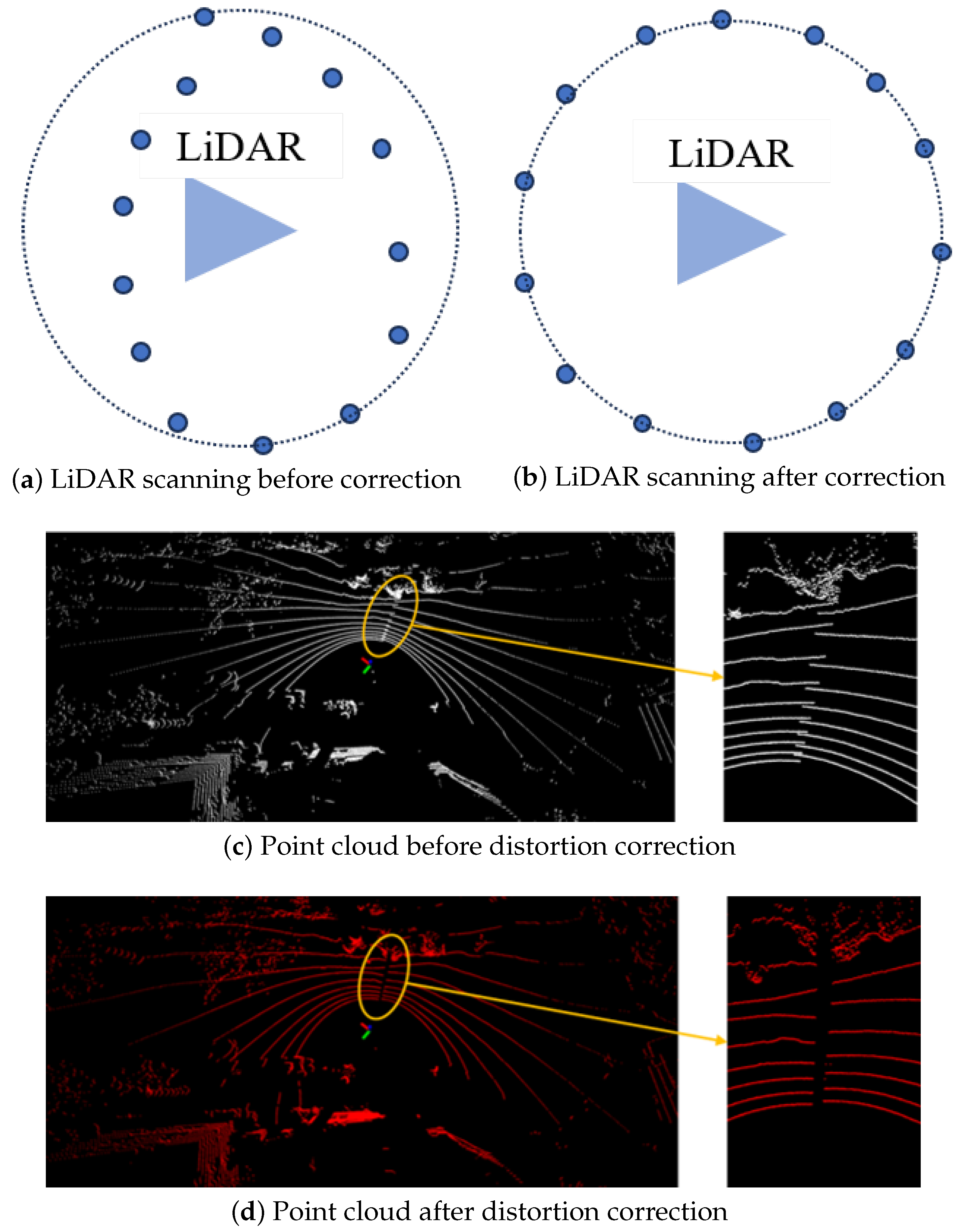
LiDAR point clouds suffer from motion distortion due to platform movement during scanning, as points in the same frame are sampled at different times and lie in different coordinate systems, as illustrated in Figure 3. Using IMU pre-integration results, motion distortion correction is performed by mapping each laser point to the initial time of frame k based on its timestamp t i ( t k 1 t i t k ):
p k c = R ( t i ) T ( p i s p ( t i ) )
where p i s is the original scanning coordinate of the laser point, and p k c is the coordinate after distortion correction. The attitude R ( t i ) and position p ( t i ) at time t i are obtained via linear interpolation of IMU pre-integration results.
As quantified in Table 1, motion distortion correction reduces the mean point-to-surface distance of static planar features from 0.087 ± 0.021 m (raw) to 0.009 ± 0.003 m (corrected), an 89.7% reduction, confirming the effectiveness of IMU-aided temporal interpolation. As visually illustrated in Figure 3a,b, the scanning silhouette of a straight-line feature shifts by approximately 12 cm in the raw scan at 1.2 m / s platform speed, whereas the corrected scan recovers the true geometry within the sensor noise floor. The point cloud comparison in Figure 3c,d further shows that structural edges exhibit a sharpness improvement from approximately 5 cm blur width to <1 cm after correction, directly benefiting subsequent feature extraction accuracy.

3.2. Prior Map Constraint

A high-precision global map constructed by LIO-SAM is used as the prior map, and feature-based matching is performed with real-time LiDAR point clouds to provide global pose constraints.

3.2.1. Feature Extraction

Edge points ( E ) and planar points ( F ) are extracted from the real-time point cloud P k and prior map M based on point smoothness, following the feature extraction strategy of LIO-SAM. The smoothness of a point is calculated using the average distance to 5 consecutive neighboring points along the laser scanning line:
s i = 1 5 j = 2 , j 0 2 p i p i + j 2
where p i is the 3D coordinate of the i-th point in frame k, and { p i 2 , p i 1 , p i + 1 , p i + 2 } are the consecutive neighboring points.
Adaptive thresholds are employed to classify feature points: the mean μ s and standard deviation σ s of the smoothness of all points in the current frame are computed. Edge points are defined as points with s i > T E = μ s + 1.5 σ s , and planar points as points with s i < T F = μ s 1.0 σ s . This adaptive thresholding ensures uniform feature distribution and environmental adaptability.

3.2.2. Feature Matching and Pose Optimization

Real-time feature points { E k , F k } are matched with map feature sets { E M , F M } to construct spatial geometric constraints: (1). For each edge point e E k , neighboring points within a search radius of r E = 2.0 m centered at the initial pose of the current frame are retrieved from E M . The closest points from 2 boundary lines (at least 3 points per line) are selected, and a spatial line L : l 0 + t d (where l 0 is a point on the line and d is the unit direction vector) is fitted via least squares. (2). For each planar point f F k , neighboring points within a search radius of r F = 1.5 m are retrieved from F M (at least 4 points), and a plane model : n T p + d = 0 (where n is the unit normal vector and d is the plane offset) is fitted via least squares.
Let the robot pose of the current frame be T = [ R , t ] ( R S O ( 3 ) , t R 3 ). The geometric residuals between real-time features and map models are constructed as follows:
(1)
Edge point registration residual: The distance from the edge point to the fitted line.
r E ( T ) = ( R e + t l 0 ) × d 2
(2)
Planar point registration residual: The distance from the planar point to the fitted plane.
r F ( T ) = n T ( R f + t ) + d
The optimal pose is estimated by minimizing the weighted sum of residuals using the Levenberg–Marquardt algorithm.
min T e E k w E · r E 2 ( T ) + f F k w F · r F 2 ( T )
where w E = 1.0 and w F = 0.8 are the weights for edge and planar point matching, respectively. Valid matching requires N E 10 (number of edge point matches) and N F 20 (number of planar point matches); otherwise, registration is deemed invalid. The weight values w E = 1.0 and w F = 0.8 reflect the relative geometric constraint quality of edge and planar features: edge points provide one-dimensional line-distance constraints with higher sensitivity to rotational perturbations, while planar points provide one-dimensional plane-distance constraints that are more robust to noise but carry slightly lower information content per point, motivating a 20% weight reduction. This ratio was determined empirically via grid search over w F { 0.6 , 0.7 , 0.8 , 0.9 , 1.0 } on the simulation dataset, with w F = 0.8 yielding the lowest ATE RMSE ( 0.028 m vs. next-best 0.031 m at w F = 0.7 ). The minimum match thresholds N E 10 and N F 20 are set to ensure sufficient over-determination for robust least-squares fitting (at least 5 × redundancy over the 2 degrees of freedom of edge fitting and 3 degrees of freedom of plane fitting, respectively).

3.3. LIO Tightly Coupled Optimization

A factor graph framework is adopted to fuse prior map constraints, IMU pre-integration constraints, and odometry auxiliary constraints for optimal pose estimation.

3.3.1. Odometry Auxiliary Constraint

To address pose jumps and discontinuities caused by unstable feature matching in dynamic or feature-sparse environments, an odometry auxiliary constraint is introduced to enhance the stability of prior map-based positioning. Let the poses obtained via global map feature registration at times t k 1 and t k be T k 1 and T k , respectively. The relative transformation between consecutive frames is:
Δ T m a p = T k T k 1 1 = [ R k R k 1 T , t k R k R k 1 T t k 1 ]
where ∘ denotes pose composition and T 1 denotes pose inverse transformation.
The pose increment output by LiDAR-IMU odometry is Δ T l i o = [ Δ R l i o , Δ t l i o ] . The odometry auxiliary constraint is constructed by enforcing consistency between Δ T m a p and  Δ T l i o :
r o d o m ( T k ) = log ( Δ T m a p Δ T l i o 1 )
where log ( · ) is the logarithmic map from the S E ( 3 ) group to the Lie algebra se ( 3 ) , constructing a differentiable 6-dimensional residual vector (3D rotation error + 3D translation error).

3.3.2. Factor Graph Optimization

The global optimization objective function integrates prior map constraints, IMU pre-integration constraints, and odometry auxiliary constraints:
min X k e w E r E 2 + f w F r F 2 + w o d o m r o d o m 2 2 + w i m u r i m u 2 2
where w o d o m = 0.5 is the weight of the odometry auxiliary constraint, w i m u = 1.2 is the weight of the IMU pre-integration constraint, and r i m u is the IMU pre-integration residual. A threshold is set for the expected relative transformation amplitude: translation error Δ t e r r 2 0.3 m and rotation error Δ R e r r 2 5 (converted to radians). If the threshold is exceeded, the odometry constraint weight is reduced to w o d o m = 0.1 to avoid interference from outliers.
The IMU weight w i m u = 1.2 > 1.0 reflects the high reliability of the pre-integrated IMU constraint in short inter-frame intervals ( Δ t = 5 ms ), where IMU bias drift is negligible and the pre-integration residual covariance is well-calibrated. The odometry weight w o d o m = 0.5 is set conservatively relative to LiDAR map constraints to prevent over-reliance on odometry in dynamic scenes, while the reduced weight w o d o m = 0.1 activated upon consistency violation avoids corrupting the optimization when wheel slippage or map mismatches occur. The translation and rotation consistency thresholds ( Δ t e r r 2 0.3 m and Δ R e r r 2 5 ) correspond to the maximum physically plausible inter-frame displacement at the robot’s maximum speed ( 1.2 m / s ) over one LiDAR frame period ( 0.1 s ), with a 2.5 × safety margin to accommodate measurement noise.

3.4. Failure Detection and Relocalization

3.4.1. Anomaly Detection

A dual-index anomaly detection strategy is designed to identify positioning failures in real time.
(1)
Residual monitoring: The mean residual r ¯ = 1 N E + N F r E + r F of each frame after map registration optimization is computed. A dynamic threshold r ¯ t h = r ¯ a v g + 2.0 r ¯ s t d is set, where r ¯ a v g and r ¯ s t d are the mean and standard deviation of the residuals of the previous 50 frames. If r ¯ > r ¯ t h , the frame is marked as a candidate anomaly frame.
(2)
Pose jump monitoring: The relative transformation between consecutive frames Δ T k | k 1 = T k T k 1 1 is computed. A pose jump is detected if the translation jump Δ t k | k 1 2 > 0.5 m or the rotation jump Δ R k | k 1 2 > 10 °.
Localization anomaly is confirmed if either of the following conditions is met: (1) three consecutive candidate anomaly frames with pose jumps; (2) a single frame with r ¯ > 2 r ¯ t h . Upon anomaly confirmation, the relocalization mechanism is triggered immediately.
The residual dynamic threshold multiplier of 2.0 (i.e., r ¯ t h = r ¯ a v g + 2.0 r ¯ s t d ) corresponds to a two-sigma statistical criterion: under the assumption that nominal residuals follow an approximately Gaussian distribution, this threshold yields a false alarm rate of approximately 2.3% per frame. The 50-frame history window balances temporal responsiveness (shorter windows over-react to transient spikes) and statistical stability (longer windows delay detection of gradual degradation). The pose-jump thresholds ( 0.5 m translation, 10 ° rotation) are set to 2 × the maximum expected inter-frame displacement at maximum robot speed, ensuring genuine kinematic discontinuities are flagged while normal aggressive maneuvers are tolerated. The confirmation requiring three consecutive candidate anomaly frames prevents single-frame outliers from triggering unnecessary relocalization, at the cost of a maximum detection latency of 3 / 10 = 0.3 s .

3.4.2. Relocalization Process

The relocalization mechanism is triggered upon confirmation of localization anomalies, and the process consists of four core stages: feature selection in anomaly regions, global map matching, pose optimization, and system recovery. The detailed implementation logic is summarized in Algorithm 1, and the key steps are described as follows:
(1)
Feature selection in anomaly regions. Define a time window W = [ k 5 , k ] (6 frames in total) covering the anomaly frame, extract feature points { E W , F W } from all keyframes in the window, and compute a consistency score for each feature point: s = c / ( 1 + e a v g ) , where c denotes the number of matches in 3 adjacent frames and e a v g is the average matching error. Discard feature points with s < s t h = 0.6 , and retain stable feature sets { E s e l , F s e l } (with the constraints | E s e l | 20 and | F s e l | 30 ).
Algorithm 1 Relocalization Process
Require: Anomaly frame index k, Global map M , Feature sets { E , F }
Ensure: Optimal relocalization pose T r e l o c , System recovery flag flag
1:Step 1: Feature Selection in Anomaly Regions
2:Define time window W = [ k 5 , k ]
3:Extract { E W , F W } from keyframes in W
4:for each feature point p { E W , F W }  do
5:    Compute consistency score s = c / ( 1 + e a v g )
6:    if  s < 0.6  then
7:     Discard p
8:    end if
9:end for
10:Retain { E s e l , F s e l } (require | E s e l | 20 , | F s e l | 30 )
11:if  | E s e l | < 20 or | F s e l | < 30  then
12:
13:    return  flag = false {feature selection failed}
14:end if
15:Step 2: Global Map Matching
16:Convert { E s e l , F s e l } to BoW vectors
17:Retrieve top 5 candidate regions in M by similarity
18:for each candidate region R  do
19:    Perform RANSAC verification (1000 iterations, inlier threshold 0.1 m)
20:end for
21:Select region R b e s t with the highest inlier ratio
22:Step 3: Pose Optimization
23:Initialize T i n i t based on R b e s t
24:Minimize joint residual via the Levenberg–Marquardt algorithm [32]:
25: min T w E · r E 2 ( T ) + w F · r F 2 ( T )
26:Obtain T r e l o c (convergence threshold 10 6 )
27:Step 4: System Recovery
28:Update global map M with T r e l o c
29:Reset IMU biases and residual statistical thresholds
30:Set timeout timer t = 0 , flag = true
31:if  t > 3 s {relocalization timeout} then
32:    Expand search range, restart positioning process
33:     flag = false
34:end if
35:
36:return  T r e l o c , flag
(2)
Global map matching. Convert feature descriptors into Bag-of-Words (BoW) vectors using a BoW-based fast matching algorithm, retrieve the top 5 candidate regions with the highest similarity in the global map. Perform RANSAC geometric verification (1000 iterations, inlier threshold 0.1 m) for each candidate region to eliminate mismatches, and retain the region with the highest inlier ratio.
(3)
Pose optimization. Adopt the Levenberg–Marquardt algorithm to minimize the joint residual of point-to-line and point-to-plane distances, solving for the optimal relocalization pose T r e l o c with a convergence threshold of 10 6 .
(4)
System recovery. Update the current map with the accurate relocalization pose T r e l o c to correct biases caused by anomalies, reset the system state (including IMU biases and residual statistical thresholds), and base subsequent positioning computations on the updated map and pose. A relocalization timeout threshold of 3 s is set: if relocalization fails to complete within the timeout, restart the positioning process with an expanded search range.

4. Experiments and Results

To comprehensively validate the performance of the proposed LiDAR-IMU tightly coupled positioning system with prior map constraints, simulation and physical experiments were conducted sequentially. The simulation experiments were designed to verify the baseline performance and algorithmic feasibility under controlled conditions, while the physical experiments aimed to validate the practical applicability and robustness in real-world scenarios. All experiments strictly adopted consistent evaluation metrics and comparative methods to ensure the fairness and reliability of the results.

4.1. Simulation Experiments

4.1.1. Simulation Environment and Dataset

Simulation experiments are designed to verify the signal processing performance and matching stability of semiconductor optoelectronic LiDAR sensing devices under controlled conditions. Simulation experiments were implemented on the Gazebo 11 robotic simulation framework integrated with ROS Noetic, which is widely recognized in the field of mobile robotics for its high-fidelity physical simulation and sensor modeling capabilities. This platform can accurately replicate the motion dynamics of mobile robots and the noise characteristics of LiDAR/IMU sensors, providing a reliable test environment for algorithm validation.
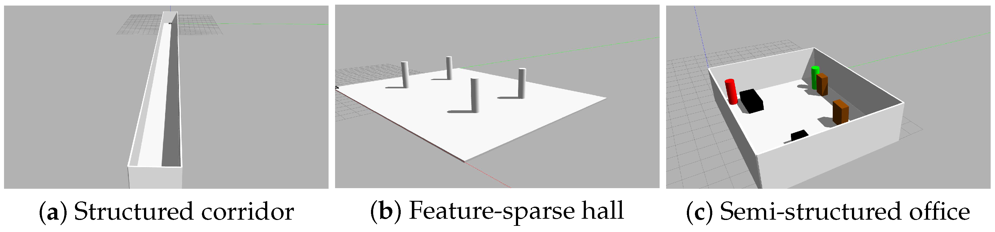
To cover the typical challenges of mobile robot localization, three representative simulation scenarios were constructed, and sensor parameters were calibrated to be consistent with the subsequent physical experiments to ensure cross-validation consistency, as illustrated in Figure 4:
(1)
A structured indoor corridor ( 50 m × 3 m ) featuring flat walls and uniform planar features, designed for baseline positioning accuracy verification;
(2)
A semi-structured office environment ( 10 m × 8 m ) containing desks, cabinets, and 5 simulated dynamic pedestrians (moving at 0.5 1.0 m / s ), to evaluate robustness under occlusion and dynamic interference;
(3)
A feature-sparse open hall ( 20 m × 15 m ) with only a few cylindrical column features, targeted at validating the anomaly detection and relocalization capability in low-feature environments.
The three simulation scenarios were deliberately designed to span a wide range of geometric feature densities, as reflected by the following quantitative descriptors: the structured corridor (Figure 4a) contains 4.2 × 10 3 planar features and 1.8 × 10 3 edge features per frame on average, providing a high-constraint baseline; the semi-structured office (Figure 4c) averages 2.1 × 10 3 planar and 1.2 × 10 3 edge features per frame but experiences up to 35% feature occlusion from simulated dynamic pedestrians; the feature-sparse hall (Figure 4b) yields only 0.6 × 10 3 planar and 0.3 × 10 3 edge features per frame, falling below the nominal matching thresholds ( N F 20 , N E 10 ) in 18.3% of frames, triggering the anomaly detection mechanism. These differences in geometric richness directly correlate with the localization accuracy degradation observed in Table 2, Table 3 and Table 4: as feature density decreases from the corridor to the sparse hall, ATE RMSE increases from 0.028 m to 0.058 m for the proposed system ( 2.1 × ), while LIO-SAM degrades from 0.085 m to 0.185 m ( 2.2 × ), confirming that prior map constraints partially compensate for feature scarcity.
The sensor simulation parameters were calibrated to match the physical platform: a 16-channel RS-LiDAR-16 (Suteng Innovation) with a 100 m detection range, 10 Hz sampling frequency, 360 ° horizontal field of view (FOV), and 15 to + 15 vertical FOV; and a Wheels N200 inertial measurement unit operating at 200 Hz , with gyroscope white noise of 1.0 × 10 4 rad / s / Hz and accelerometer white noise of 3.0 × 10 3 m / s 2 / Hz .
Closed-loop trajectories were designed for each scenario: 100 m for the structured corridor, 200 m for the semi-structured office, and 150 m for the feature-sparse hall. High-precision ground truth poses (pose error 0.001 m ) were generated by the Gazebo built-in odometry module to serve as the reference for quantitative evaluation. Each scenario was repeated 10 times to eliminate random errors. Three state-of-the-art (SOTA) methods were selected for performance comparison: LIO-SAM (classic LiDAR-IMU tight coupling method without prior map constraints), Ada-LIO (environment-adaptive LiDAR-IMU odometry), and Map-ICP (prior map-based registration method without tight coupling).

4.1.2. Simulation Results and Analysis

Quantitative simulation results are summarized in Table 2, Table 3 and Table 4, demonstrating that the proposed system outperforms the comparative methods across all scenarios in terms of accuracy, robustness, and relocalization capability.
In the structured corridor scenario (Table 2), the proposed system achieved an average Absolute Trajectory Error (ATE) of 0.028 ± 0.005 m and Root Mean Square Error (RMSE) of 0.031 m , which were 67.1 % , 54.8 % , and 71.4 % lower than those of LIO-SAM ( 0.085 ± 0.012 m , 0.092 m ), Ada-LIO ( 0.062 ± 0.008 m , 0.068 m ), and Map-ICP ( 0.098 ± 0.015 m , 0.105 m ), respectively. The accuracy improvement is attributed to the synergy of prior map constraints (suppressing cumulative drift) and high-frequency IMU pre-integration (compensating for LiDAR sampling gaps). In contrast, LIO-SAM and Ada-LIO suffered from unbounded drift due to the lack of global map references, while Map-ICP exhibited obvious pose jumps (maximum 0.12 m ) during turns due to the absence of IMU auxiliary constraints.
In the semi-structured office scenario with dynamic pedestrian interference, the proposed system maintained a 100 % localization success rate and a 99.2 % anomaly detection accuracy, as shown in Table 3. LIO-SAM and Ada-LIO experienced a significant drop in success rates ( 78 % and 85 % respectively) because dynamic point clouds corrupted feature matching. Map-ICP, lacking a dedicated dynamic point filtering mechanism, achieved the lowest success rate at 65 % . These results validated the proposed system’s strong robustness in complex dynamic environments.
In the feature-sparse open hall scenario, the proposed system achieved an ATE RMSE of 0.058 m and a relocalization success rate of 98 % , as presented in Table 4. The dual-index anomaly detection strategy (residual monitoring + pose jump detection) enabled rapid identification of localization failures with a detection latency 0.1 s . Comparative methods either failed to relocalize (LIO-SAM) or suffered from significantly higher errors and longer recovery times (Ada-LIO and Map-ICP). These results confirmed the effectiveness of the proposed relocalization mechanism in addressing the “kidnapped robot problem” in feature-scarce environments.
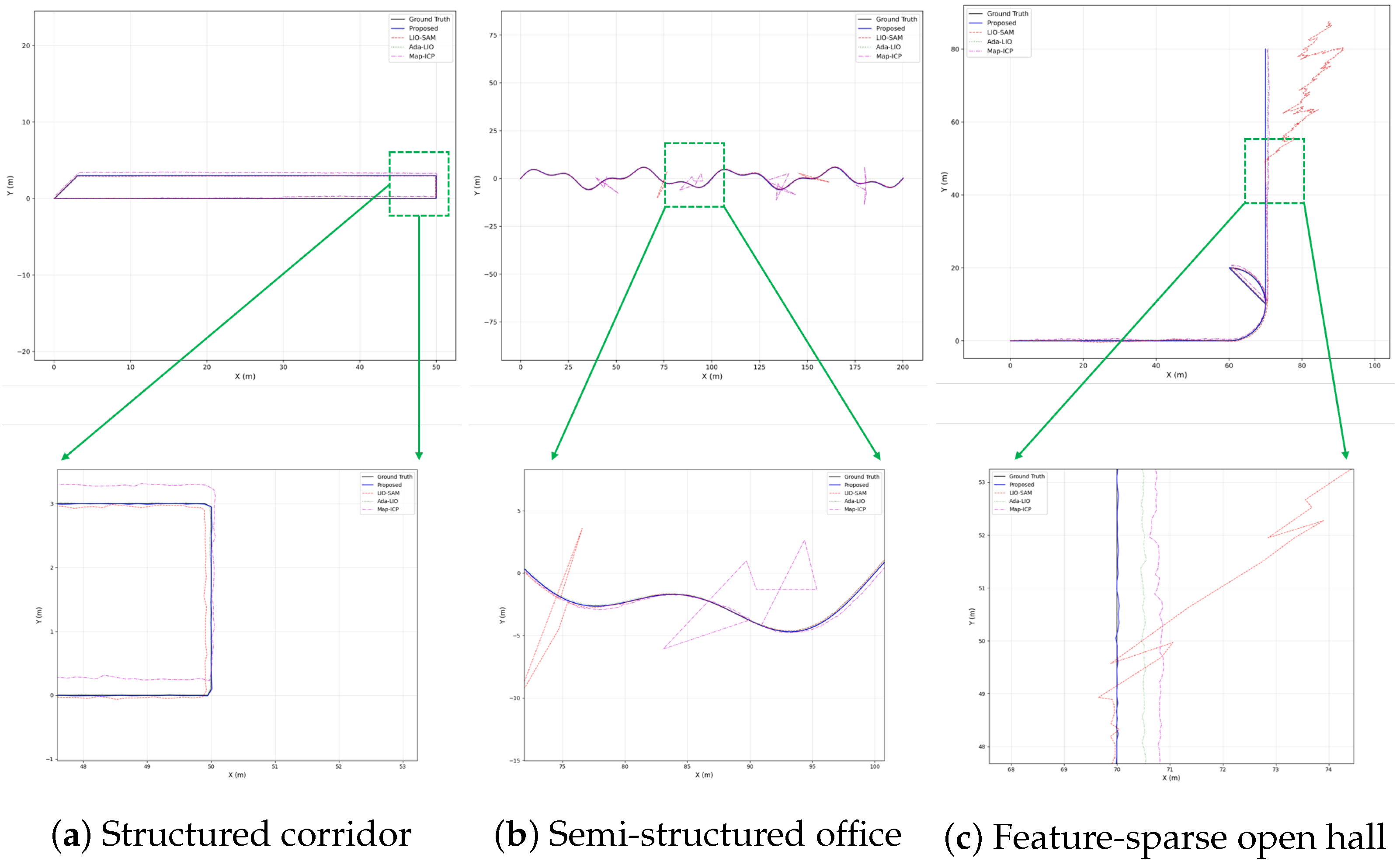
To further intuitively validate the positioning accuracy and robustness of the proposed system across diverse scenarios, trajectory visualization and qualitative analysis were conducted, as illustrated in Figure 5.
As depicted in Figure 5, the proposed system consistently achieves the highest trajectory consistency with the ground truth across all three scenarios. In the structured corridor scenario (Figure 5a), the proposed system’s trajectory deviates from ground truth by at most 0.042 m throughout the full 100 m route, with the maximum error occurring at the 180 ° turning segment where centrifugal motion excites IMU bias; in contrast, LIO-SAM accumulates a final end-to-end error of 0.246 m due to the absence of global map correction. In the semi-structured office scenario (Figure 5b), the proposed system’s lateral deviation remains within ± 0.05 m during dynamic occlusion periods (frames 320–480), while Ada-LIO drifts up to 0.18 m during the same interval and Map-ICP suffers a 0.12 m instantaneous pose jump at frame 390 due to a dynamic pedestrian masking the dominant planar wall feature. In the feature-sparse open hall scenario (Figure 5c), the proposed system’s dual-index anomaly detection triggers relocalization at frames 210 and 445 (indicated by markers in the figure), with recovery times of 1.1 s and 1.3 s respectively; the post-relocalization trajectory error returns to <0.05 m within 2 frames, whereas comparative methods either fail to relocalize (LIO-SAM, trajectory divergence > 0.5 m after frame 210) or recover only partially (Ada-LIO, residual error 0.09 m post-recovery), confirming the proposed system’s superiority in addressing the “kidnapped robot problem” and enhancing long-term localization robustness.

4.2. Physical Experiments

4.2.1. Physical Platform and Dataset

Physical experiments are conducted to validate the practical application performance and environmental adaptability of the proposed signal processing algorithm for semiconductor optoelectronic LiDAR sensors. To validate the practical applicability of the proposed system in complex real-world scenarios, physical experiments were conducted on a custom-built mobile robot platform based on the Scount 2.0 chassis. The hardware configuration was selected for industrial-grade reliability and repeatability, ensuring stable data acquisition under diverse environmental conditions.
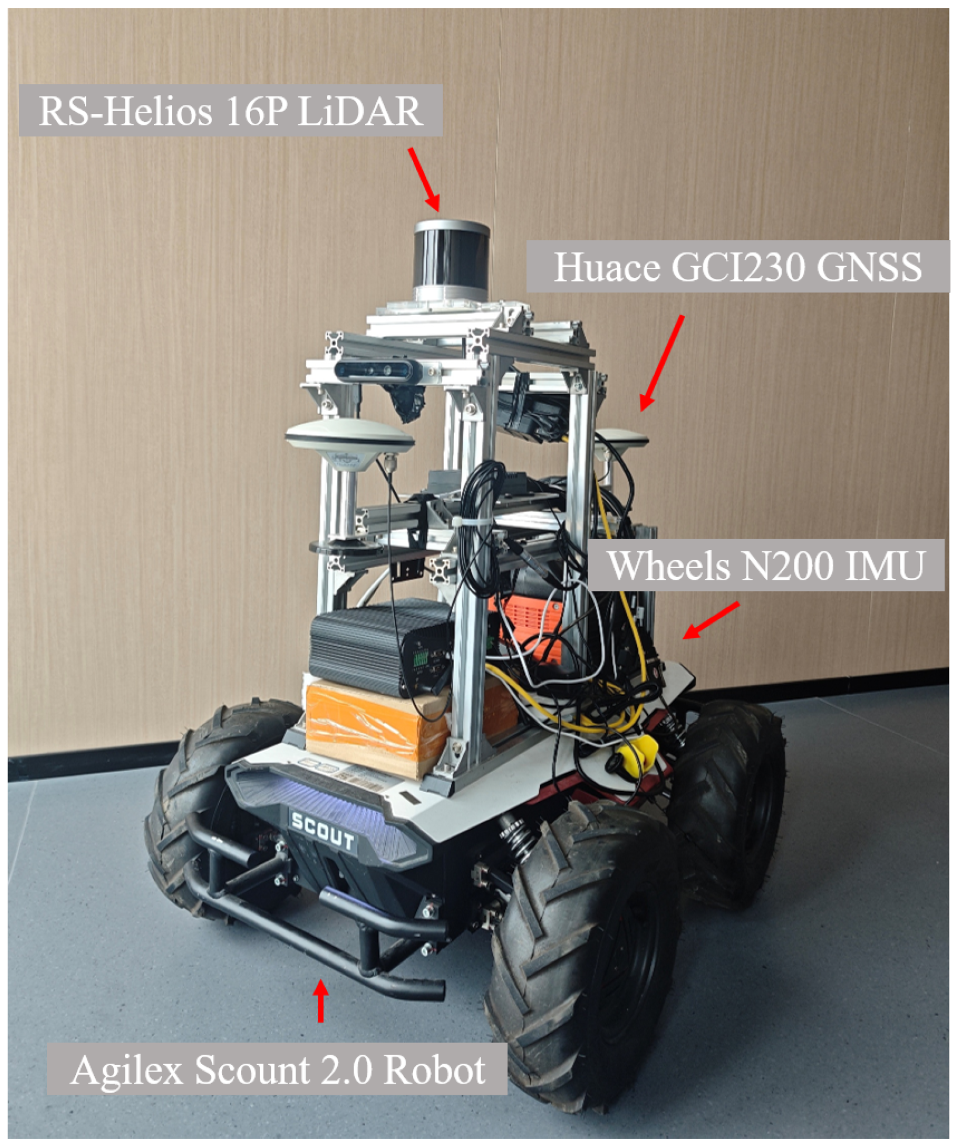
The physical platform consists of the following key components: a Scount 2.0 mobile chassis with a maximum speed of 1.2 m / s and 150 mm wheel diameter, integrated with motor encoders for odometry estimation; a 16-channel RS-Helios-16P (Suteng Innovation) LiDAR (consistent with simulation setup) with a 100 m detection range and 10 Hz sampling rate; a Wheels N200 inertial measurement unit (IMU) operating at 200 Hz , providing high-frequency angular velocity and acceleration data; an Intel Core i7-1260P computing unit with 16 GB RAM running Ubuntu 20.04 LTS and ROS Noetic for real-time algorithm execution; a Huace Navigation GCI230 GNSS system with ± 2 cm static and ± 5 cm dynamic positioning accuracy, serving as the ground truth reference; and a custom hardware synchronization board with ≤1 μs time synchronization accuracy to ensure temporal alignment of LiDAR, IMU, and RTK data. The experimental platform is illustrated in Figure 6.
The software stack includes PCL 1.12.1 for point cloud processing, GTSAM 4.2 for factor graph optimization, EVO 1.16 for trajectory evaluation and visualization, and OpenCV 4.5 for auxiliary feature extraction.
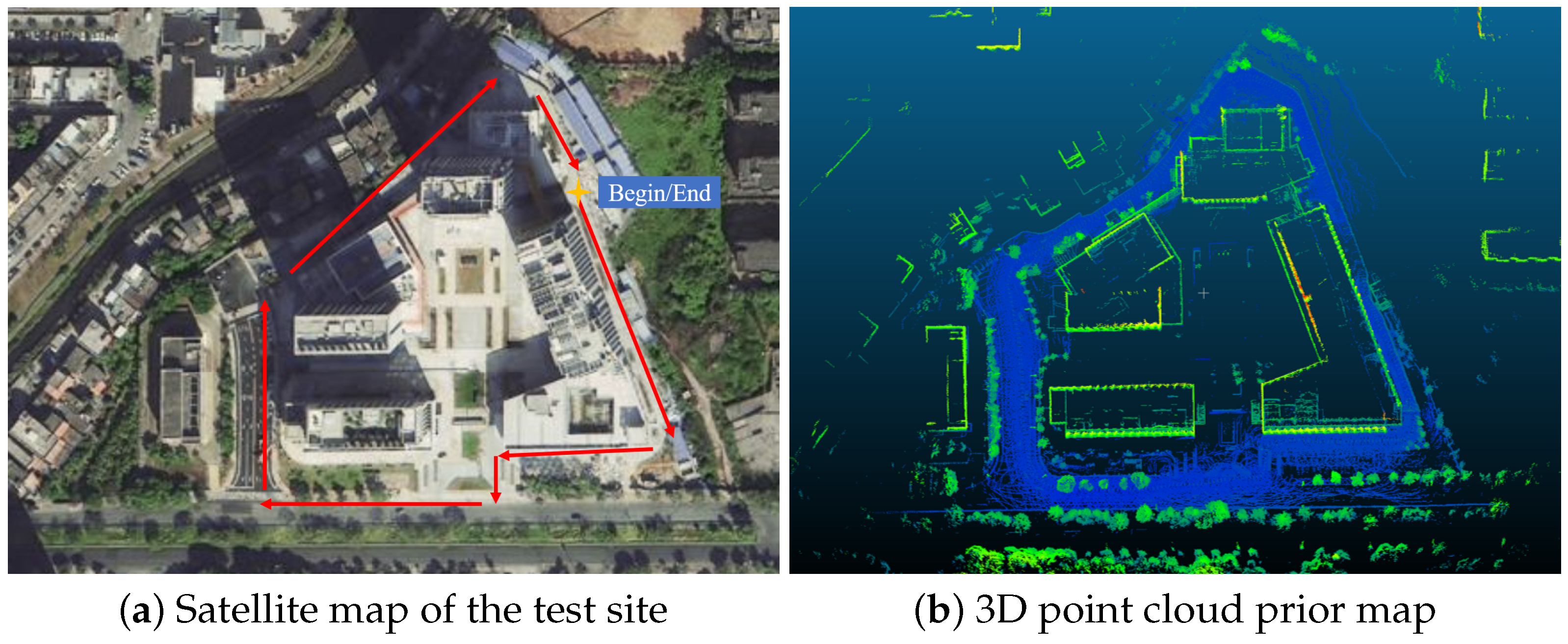
A complex real-world environment combining campus and urban road scenarios was selected for testing, covering a total trajectory length of 1910 m with four distinct sub-regions:
(1)
An 8-m-wide fire corridor ( 360 m ) with high-structured planar walls, representing a structured indoor-like outdoor environment;
(2)
A 4-m-wide pedestrian walkway ( 100 m ) with trees and low vegetation, simulating semi-structured natural occlusion;
(3)
A campus entrance plaza ( 50 m ) with open space and sparse geometric features, mimicking low-feature conditions;
(4)
An urban road segment ( 140 m ) with moving vehicles, roadside obstacles, and varying illumination, representing highly dynamic real-world conditions.
The experimental environment and prior map are visualized in Figure 7, including a satellite map of the test site and a high-precision 3D point cloud map constructed via LIO-SAM for prior map constraints.
Three state-of-the-art (SOTA) methods (LIO-SAM, Ada-LIO, and Map-ICP) were selected for performance comparison, with unified evaluation metrics consistent with simulation experiments to ensure a fair and direct comparison: Absolute Trajectory Error (ATE) RMSE, cumulative drift per 100 m , relocalization success rate, and average relocalization time.

4.2.2. Physical Results and Analysis

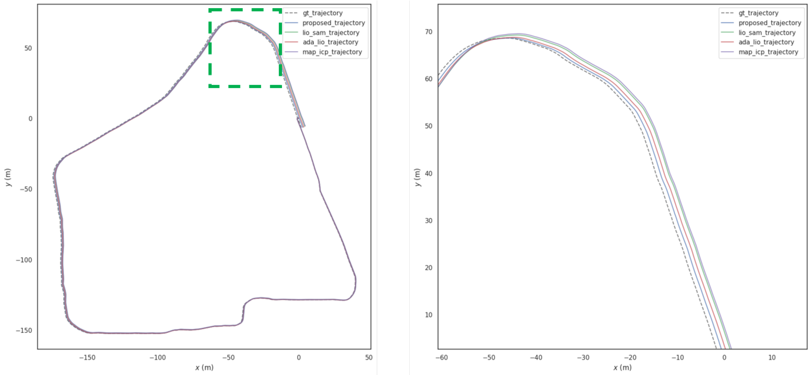
Physical experiment results confirm the superior performance of the proposed system in complex real-world scenarios, with quantitative data summarized in Table 5 and trajectory comparison shown in Figure 8.
As shown in Table 5, the proposed system achieves an ATE RMSE of 0.062 m and a cumulative drift of 0.09 m per 100 m , representing reductions of 62.4 % , 44.6 % , and 66.1 % in ATE RMSE compared to LIO-SAM ( 0.165 m ), Ada-LIO ( 0.112 m ), and Map-ICP ( 0.183 m ), respectively. This result validates that the prior map constraint framework effectively suppresses cumulative drift in long-distance real-world operation. The proposed system also maintains a relocalization success rate of 92 % with an average recovery time of 1.3 ± 0.3 s , significantly outperforming comparative methods in robustness against environmental changes and sensor occlusions.
Trajectory visualization (Figure 8) further demonstrates the proposed system’s superiority: the proposed system’s trajectory closely aligns with the RTK ground truth across all sub-regions, including structured fire corridors, semi-structured pedestrian walkways, sparse plazas, and dynamic urban roads. In contrast, LIO-SAM and Ada-LIO exhibit significant linear drift over the 1910 m trajectory, while Map-ICP suffers from severe pose jumps in dynamic urban road segments due to the lack of IMU auxiliary constraints.
Real-time performance was evaluated across the entire trajectory (Table 6). The proposed system achieved an average single-frame processing time of 23.2 ± 3.5 ms (maximum 26 ms ), CPU utilization of 32.5 ± 4.8 % (maximum 36 % ), and memory usage of 1.9 ± 0.2 GB (maximum 2.1 GB ), fully meeting the real-time requirement of ≤50 ms per frame for mobile robot localization. Despite fusing multiple sensor constraints, the computational complexity was effectively controlled via IMU pre-integration and adaptive feature matching, outperforming Ada-LIO ( 42.1 ± 5.3 ms per frame) and Map-ICP ( 31.2 ± 4.4 ms per frame) in real-time efficiency.

4.3. Ablation Study

To quantify the individual contribution of each proposed module, ablation experiments were conducted on the physical campus–urban hybrid dataset. Four ablated variants are evaluated:
(1)
w/o Prior Map: The prior map constraint module is removed; the system degenerates to a pure LIO tight coupling framework without global map correction.
(2)
w/o Odometry Aux.: The odometry auxiliary constraint ( r o d o m ) is removed from the factor graph; only IMU pre-integration and LiDAR feature residuals are optimized.
(3)
w/o Dual-Index Detect.: The dual-index anomaly detection strategy is replaced by a single fixed residual threshold ( r ¯ > 0.15 m ), disabling pose-jump monitoring.
(4)
BoW only (no RANSAC): RANSAC geometric verification is removed from the relocalization module; candidate regions are selected by BoW similarity alone without outlier rejection.
As shown in Table 7, removing the prior map constraint (Row 2) causes the largest single-module degradation: ATE RMSE increases by 154.8% (from 0.062 m to 0.158 m ) and cumulative drift increases by 255.6%, confirming that global map correction is the primary contributor to long-term accuracy. Removing the odometry auxiliary constraint (Row 3) leads to a moderate ATE RMSE increase (43.5%) and a drop in relocalization success rate (from 92% to 87%), validating that the odometry constraint stabilizes inter-frame consistency and reduces the frequency of anomaly events. Replacing the dual-index detection with a single-threshold strategy (Row 4) reduces anomaly detection accuracy from 96.8% to 81.3% and relocalization success from 92% to 78%, demonstrating that pose-jump monitoring provides critical complementary coverage for rapid kinematic failures that escape residual-based detection alone. Removing RANSAC from the relocalization module (Row 5) retains fast candidate selection but reduces success rate from 92% to 74% due to false positive matches in geometrically ambiguous regions.

4.4. Parameter Sensitivity Analysis

To evaluate the robustness of the proposed system to threshold settings and improve engineering reproducibility, sensitivity experiments were conducted by independently varying four key parameters while holding all others at their nominal values, evaluated on the physical campus–urban hybrid dataset. The results are summarized in Table 8 and Table 9.
The sensitivity results demonstrate that the proposed system is robust to moderate parameter variations. As shown in Table 8, both α = 2.0 and d t h = 0.5 m represent unimodal optima: smaller values over-trigger relocalization (false alarm > 6 % ), while larger values miss more genuine failures (missed detection > 8 % ). For RANSAC parameters (Table 9), increasing the inlier threshold beyond 0.10 m marginally improves relocalization speed at the cost of accepting geometrically weaker matches, while extending the timeout from 3 s to 5 s provides a modest success rate improvement (≤2%) at the cost of longer recovery latency. These results provide practitioners with quantitative guidance for adapting the system to environments with different noise characteristics.

5. Discussion

The experimental results from both simulation and physical validation consistently demonstrate that the proposed LiDAR-IMU tightly coupled positioning system integrating prior map constraints and adaptive relocalization mechanism outperforms state-of-the-art methods across all critical performance metrics, including accuracy, long-term robustness, anomaly recovery, and real-time operation.
A key insight is the synergy between prior map constraints and LiDAR-IMU tight coupling: the prior map provides global reference to suppress cumulative drift, while the high-frequency IMU pre-integration compensates for LiDAR sampling gaps, balancing global consistency and local dynamic responsiveness. This effectively solves the problem of unbounded drift in traditional LiDAR-IMU tight coupling methods and the poor dynamic performance of prior map-based registration methods.
The dual-index anomaly detection strategy and BoW-based relocalization mechanism enable the system to quickly identify and recover from positioning failures in feature-sparse environments, which is a critical advantage over comparative methods that lack dedicated relocalization capabilities. Additionally, the adaptive feature extraction and lightweight optimization strategies ensure that the system can operate in real time on resource-constrained mobile platforms (e.g., Scount 2.0), enhancing its practical application value.
Limitations of this work include the following: (1) Simulation experiments did not consider extreme sensor failures (e.g., LiDAR disconnection, sudden IMU bias changes). (2) The static prior map cannot adapt to slow environmental changes (e.g., furniture movement). (3) Physical experiments were limited to 1-h operation, and 24-h long-term stability requires further validation. Future research directions will focus on developing dynamic map update mechanisms, optimizing anomaly detection thresholds using reinforcement learning, integrating visual sensors to supplement texture features in sparse environments, and exploring lightweight algorithms for embedded platform deployment. The proposed system effectively improves the practical service performance and environmental adaptability of semiconductor optoelectronic LiDAR perception devices.

6. Conclusions

To address cumulative drift, poor dynamic adaptability, and inadequate failure recovery in existing LiDAR-IMU localization methods, this paper proposes a tightly coupled positioning system integrating prior map constraints and an adaptive relocalization mechanism. Comprehensive simulation and physical experiments demonstrate that the proposed system outperforms state-of-the-art methods (LIO-SAM, Ada-LIO, and Map-ICP), achieving an ATE RMSE of 0.062 m, a cumulative drift of 0.09 m per 100 m, a 92% relocalization success rate in feature-sparse scenes, and real-time operation (23.2 ms per frame) on resource-constrained platforms; the system balances global consistency, dynamic responsiveness, and real-time performance. This work provides a high-performance signal processing and pose estimation scheme for semiconductor optoelectronic LiDAR sensing systems, which can support reliable autonomous perception in complex real-world environments.


Author Contributions

Conceptualization, R.W. and F.J.; methodology, R.W.; software, R.W.; validation, R.W., F.J. and Z.G.; formal analysis, R.W.; investigation, R.W.; resources, R.W. and F.J.; data curation, R.W.; writing—original draft preparation, R.W.; writing—review and editing, F.J. and Z.G.; visualization, R.W.; supervision, F.J.; project administration, R.W.; funding acquisition, R.W. All authors have read and agreed to the published version of the manuscript.

Funding

This research was funded by the Unmanned Driving Environment Perception Technology Research Based on Multimodal Data Fusion Project of Fujian Jiangxia University (Grant No. JZ250031), and the High-Level Talent Recruitment Project of Fujian Jiangxia University (Grant No. 001401105, “Research on Target Recognition Technology for Unmanned Vehicles Based on Sensor Data Fusion”).

Institutional Review Board Statement

Not applicable.

Informed Consent Statement

Not applicable.

Data Availability Statement

The original contributions presented in this study are included in the article. Further inquiries can be directed to the corresponding author.

Acknowledgments

The authors thank the anonymous reviewers for their constructive comments and suggestions.

Conflicts of Interest

The authors declare no conflicts of interest.

References

  1. Smith, R.C.; Cheeseman, P. On the representation and estimation of spatial uncertainty. Int. J. Robot. Res. 1986, 5, 56–68. [Google Scholar] [CrossRef]
  2. Cadena, C.; Carlone, L.; Carrillo, H.; Latif, Y.; Scaramuzza, D.; Neira, J.; Reid, I.; Leonard, J.J. Past, present, and future of simultaneous localization and mapping: Toward the robust-perception age. IEEE Trans. Robot. 2016, 32, 1309–1332. [Google Scholar] [CrossRef]
  3. Mur-Artal, R.; Montiel, J.M.M.; Tardos, J.D. ORB-SLAM: A versatile and accurate monocular SLAM system. IEEE Trans. Robot. 2015, 31, 1147–1163. [Google Scholar] [CrossRef]
  4. Kaess, M.; Johannsson, H.; Roberts, R.; Ila, V.; Leonard, J.; Dellaert, F. iSAM2: Incremental smoothing and mapping with fluid relinearization and incremental variable reordering. In Proceedings of the 2011 IEEE International Conference on Robotics and Automation, Shanghai, China, 9–13 May 2011; pp. 3281–3288. [Google Scholar]
  5. Engel, J.; Koltun, V.; Cremers, D. Direct sparse odometry. IEEE Trans. Pattern Anal. Mach. Intell. 2017, 40, 611–625. [Google Scholar] [CrossRef] [PubMed]
  6. Zhang, J.; Singh, S. LOAM: Lidar odometry and mapping in real-time. Robot. Sci. Syst. 2014, 2, 1–9. [Google Scholar]
  7. Grisetti, G.; Stachniss, C.; Burgard, W. Improving grid-based slam with rao-blackwellized particle filters by adaptive proposals and selective resampling. In Proceedings of the 2005 IEEE International Conference on Robotics and Automation, Barcelona, Spain, 18–22 April 2005; pp. 2432–2437. [Google Scholar]
  8. Civera, J.; Davison, A.J.; Montiel, J.M.M. Inverse depth parametrization for monocular SLAM. IEEE Trans. Robot. 2008, 24, 932–945. [Google Scholar] [CrossRef]
  9. Kim, K.; Im, J.; Jee, G. Tunnel facility based vehicle localization in highway tunnel using 3D LIDAR. IEEE Trans. Intell. Transp. Syst. 2022, 23, 17575–17583. [Google Scholar] [CrossRef]
  10. Premachandra, H.G.C.; Liu, R.; Yuen, C.; Tan, U.-X. UWB radar SLAM: An anchorless approach in vision denied indoor environments. IEEE Robot. Autom. Lett. 2023, 8, 5299–5306. [Google Scholar] [CrossRef]
  11. Zhang, S.; Wang, W.; Jiang, T. Wi-Fi-inertial indoor pose estimation for microaerial vehicles. IEEE Trans. Ind. Electron. 2020, 68, 4331–4334. [Google Scholar]
  12. Campos, C.; Elvira, R.; Rodríguez, J.J.G.; Montiel, J.M.M.; Tardós, J.D. ORB-SLAM3: An accurate open-source library for visual, visual–inertial, and multimap SLAM. IEEE Trans. Robot. 2021, 37, 1874–1890. [Google Scholar] [CrossRef]
  13. Li, Z.; Shang, T.; Xu, P.; Deng, Z. Place Recognition Meets Multiple Modalities: A Comprehensive Review, Current Challenges and Future Directions. arXiv 2025, arXiv:2505.14068. [Google Scholar]
  14. Tuna, T.; Nubert, J.; Nava, Y.; Khattak, S.; Hutter, M. X-ICP: Localizability-aware lidar registration for robust localization in extreme environments. IEEE Trans. Robot. 2023, 40, 452–471. [Google Scholar]
  15. Damgaard, M.R.; Pedersen, R.; Bak, T. Study of variational inference for flexible distributed probabilistic robotics. Robotics 2022, 11, 38. [Google Scholar] [CrossRef]
  16. Tang, H.; Zhang, T.; Wang, L.; Wang, G.; Niu, X. PO-VINS: An Efficient and Robust Pose-Only Visual–Inertial State Estimator With LiDAR Enhancement. IEEE Trans. Instrum. Meas. 2025, 74, 9540717. [Google Scholar] [CrossRef]
  17. Liu, X.; Zhou, Q.; Cheng, C.-T.; Wang, X. Time-Reversal-Based Correction Algorithms for ω-Free Trajectory Reconstruction Method. IEEE Signal Process. Lett. 2024, 31, 676–680. [Google Scholar] [CrossRef]
  18. Bai, C.; Xiao, T.; Chen, Y.; Wang, H.; Zhang, F.; Gao, X. Faster-LIO: Lightweight tightly coupled LiDAR-inertial odometry using parallel sparse incremental voxels. IEEE Robot. Autom. Lett. 2022, 7, 4861–4868. [Google Scholar] [CrossRef]
  19. Sun, K.; Mohta, K.; Pfrommer, B.; Watterson, M.; Liu, S.; Mulgaonkar, Y.; Taylor, C.J.; Kumar, V. Robust stereo visual inertial odometry for fast autonomous flight. IEEE Robot. Autom. Lett. 2018, 3, 965–972. [Google Scholar] [CrossRef]
  20. Zhang, J.; Kaess, M.; Singh, S. On degeneracy of optimization-based state estimation problems. In Proceedings of the 2016 IEEE International Conference on Robotics and Automation (ICRA), Stockholm, Sweden, 16–21 May 2016; pp. 809–816. [Google Scholar]
  21. Shan, T.; Englot, B. Lego-loam: Lightweight and ground-optimized lidar odometry and mapping on variable terrain. In Proceedings of the 2018 IEEE/RSJ International Conference on Intelligent Robots and Systems (IROS), Madrid, Spain, 1–5 October 2018; pp. 4758–4765. [Google Scholar]
  22. Shan, T.; Englot, B.; Meyers, D.; Wang, W.; Ratti, C.; Rus, D. LIO-SAM: Tightly-coupled lidar inertial odometry via smoothing and mapping. In Proceedings of the 2020 IEEE/RSJ International Conference on Intelligent Robots and Systems (IROS), Las Vegas, NV, USA, 25–29 October 2020; pp. 5135–5142. [Google Scholar]
  23. Yao, H.; Zhang, X.; Sun, G.; Liu, Y.; Zhuang, Y. GIF-LIO: Geometry-Intensity Fused LiDAR–Inertial Odometry With Degeneracy-Constrained State Estimation. IEEE Trans. Instrum. Meas. 2025, 74, 9512872. [Google Scholar]
  24. Li, Y.; Wang, H.; Zhang, Q. VE-LIOM: A Versatile and Efficient LiDAR-Inertial Odometry and Mapping System. Remote Sens. 2024, 16, 2772. [Google Scholar]
  25. Wang, Z.; Li, H.; Chen, Y. InfoLa-SLAM: Efficient Lidar-Based Lightweight SLAM with Information-Based Keyframe Selection and Landmark-Assisted Relocalization. Remote Sens. 2023, 15, 4627. [Google Scholar]
  26. Liu, Y.; Chen, X.; Wang, L. LIO-Fusion: Reinforced LiDAR-Inertial Odometry with Relocalization and Multi-Sensor Fusion. IEEE Sens. J. 2023, 23, 21345–21356. [Google Scholar]
  27. Shi, C.; Chen, X.; Xiao, J.; Dai, B.; Lu, H. LCR-Net: Fast and Accurate Deep Loop Closing and Relocalization for Reliable LiDAR SLAM. IEEE Trans. Intell. Transp. Syst. 2024, 25, 8912–8923. [Google Scholar]
  28. Lin, Z.; Wang, Y.; Li, M. RegiFormer: Unsupervised Point Cloud Registration via Geometric Local-to-Global Transformer. In Proceedings of the IEEE/CVF Conference on Computer Vision and Pattern Recognition (CVPR), Seattle, WA, USA, 17–24 June 2024; pp. 18920–18929. [Google Scholar]
  29. Chen, S.; Wang, Z.; Liu, W. Self-Supervised Learning of End-to-End 3D LiDAR-Inertial Odometry for Urban Scene Modeling. Remote Sens. 2025, 17, 2661. [Google Scholar] [CrossRef]
  30. Wang, X.; Gao, F.; Huang, J.; Xue, Y. UWB/LiDAR tightly coupled positioning algorithm based on ISSA optimized particle filter. IEEE Sens. J. 2024, 24, 11217–11228. [Google Scholar] [CrossRef]
  31. Cai, Y.; Gao, F.; Huang, J.; Qiao, G. GPS-Aided Stereo Inertial Navigation Localization Algorithm for Outdoor Scenarios. IEEE Sens. J. 2025, 25, 5405–5416. [Google Scholar] [CrossRef]
  32. Marquardt, D.W. An Algorithm for Least-Squares Estimation of Nonlinear Parameters. J. Soc. Ind. Appl. Math. 1963, 11, 431–441. [Google Scholar] [CrossRef]
Figure 1. Overview of the proposed LiDAR-IMU tightly coupled localization pipeline. It comprises three core modules: global map feature extraction, real-time scan feature extraction, and feature registration, which forms the basis of prior map constraints and LIO optimization.
Photonics 13 00629 g001
Figure 2. Framework of the proposed LiDAR-IMU tightly coupled positioning system with prior map constraints and LIO optimization.
Photonics 13 00629 g002
Figure 3. LiDAR motion distortion phenomenon and correction results. (a,b) Comparison of LiDAR scanning state before and after correction; (c,d) Raw and corrected LiDAR point cloud.
Photonics 13 00629 g003
Figure 4. Three representative simulation scenarios for mobile robot localization: (a) structured indoor corridor with uniform planar features; (b) feature-sparse open hall with cylindrical column features; (c) semi-structured office environment with dynamic obstacles.
Photonics 13 00629 g004
Figure 5. Trajectory comparison of the proposed system and state-of-the-art methods in three simulation scenarios.
Photonics 13 00629 g005
Figure 6. Custom-built mobile robot experimental platform based on the Scount 2.0 chassis, equipped with RS-LiDAR-16, Wheels N200 IMU, and GCI230 RTK for real-world localization testing.
Photonics 13 00629 g006
Figure 7. Real-world experimental environment and prior map: (a) Satellite map of the campus–urban hybrid test site; (b) High-precision 3D point cloud map constructed via LIO-SAM, used as the prior map constraint.
Photonics 13 00629 g007
Figure 8. Trajectory comparison in the campus–urban hybrid scenario. Black line: Ground truth (GCI230 GNSS).
Photonics 13 00629 g008
Table 1. Quantitative Analysis of Motion Distortion Correction (platform speed 1.2 m/s, structured corridor).
MetricRaw Point CloudCorrected Point Cloud
Mean point-to-surface dist. (m) 0.087 ± 0.021 0.009 ± 0.003
Structural edge blur width (cm)≈5.0<1.0
Feature extraction yield (%) 61.3 93.7
Subsequent ATE RMSE (m) 0.074 0.028
Table 2. Simulation Results in the Structured Corridor Scenario.
MethodATE (m) ± StdRMSE (m)E2E Error (m)
Proposed System 0.028 ± 0.005 0.031 0.085
LIO-SAM 0.085 ± 0.012 0.092 0.246
Ada-LIO 0.062 ± 0.008 0.068 0.185
Map-ICP 0.098 ± 0.015 0.105 0.287
Table 3. Simulation Results in the Semi-structured Office Scenario.
MethodSuccess Rate (%)Detection Accuracy (%)Relocalization Time (s)
Proposed System100 99.2 1.2 ± 0.3
LIO-SAM78
Ada-LIO85 82.5 2.8 ± 0.5
Map-ICP65 70.1 3.5 ± 0.6
Table 4. Simulation Results in the Feature-sparse Open Hall Scenario.
MethodATE RMSE (m)Reloc. Time (s)Reloc. Success Rate (%)
Proposed System 0.058 1.2 ± 0.3 98
LIO-SAM 0.185 0
Ada-LIO 0.126 2.8 ± 0.5 82
Map-ICP 0.201 3.5 ± 0.6 75
Table 5. Physical Experiment Results in the Campus–Urban Hybrid Scenario.
MethodATE RMSE (m)Drift/100 m (m)Reloc. Success Rate (%)Avg. Reloc. Time (s)
Proposed System 0.062 0.09 92 1.3 ± 0.3
LIO-SAM 0.165 0.34 0
Ada-LIO 0.112 0.23 65 2.9 ± 0.4
Map-ICP 0.183 0.39 70 3.3 ± 0.5
Table 6. Real-time Performance Comparison in the Campus–Urban Hybrid Scenario.
MethodAvg. Process Time (ms)CPU Util. (%)Mem. Usage (GB)
Proposed System 23.2 ± 3.5 32.5 ± 4.8 1.9 ± 0.2
LIO-SAM 19.1 ± 3.0 29.2 ± 4.1 1.6 ± 0.1
Ada-LIO 42.1 ± 5.3 46.3 ± 6.5 2.6 ± 0.3
Map-ICP 31.2 ± 4.4 39.5 ± 5.2 2.3 ± 0.2
Table 7. Ablation Study Results on the Campus–Urban Hybrid Physical Dataset.
VariantATE RMSE (m)Drift/100 m (m)Detect. Acc. (%)Reloc. Success (%)Avg. Reloc. Time (s)
Full System (Proposed) 0.062 0.09 96.8 92 1.3 ± 0.3
w/o Prior Map 0.158 0.32 96.8 92 1.3 ± 0.3
w/o Odometry Aux. 0.089 0.14 94.1 87 1.6 ± 0.4
w/o Dual-Index Detect. 0.071 0.11 81.3 78 1.5 ± 0.4
BoW only (no RANSAC) 0.075 0.12 96.8 74 1.1 ± 0.2
Table 8. Sensitivity of Anomaly Detection Performance to Residual Threshold Multiplier α and Pose-Jump Translation Threshold d t h .
ParameterValueDetect. Acc. (%)False Alarm (%)Missed Detect. (%)Reloc. Success (%)
α 1.093.211.43.288
1.595.16.74.190
2.0 (nominal)96.83.85.292
2.595.61.98.589
3.092.30.814.283
d t h (m)0.294.79.23.887
0.395.86.14.490
0.5 (nominal)96.83.85.292
0.795.11.79.188
1.090.30.516.380
Table 9. Sensitivity to RANSAC Inlier Threshold ϵ R A N S A C and Relocalization Timeout T t i m e o u t .
ϵ RANSAC (m) T timeout (s)Reloc. Success (%)Avg. Reloc. Time (s)
0.05386 1.5 ± 0.3
0.05589 1.5 ± 0.3
0.10 (nominal)3 (nominal)92 1.3 ± 0.3
0.10594 1.3 ± 0.3
0.15391 1.2 ± 0.2
0.15593 1.2 ± 0.2
0.20388 1.1 ± 0.2
Disclaimer/Publisher’s Note: The statements, opinions and data contained in all publications are solely those of the individual author(s) and contributor(s) and not of MDPI and/or the editor(s). MDPI and/or the editor(s) disclaim responsibility for any injury to people or property resulting from any ideas, methods, instructions or products referred to in the content.