Research on Power Laser Inspection Technology Based on High-Precision Servo Control System

Abstract

With the expansion of the scale of ultra-high-voltage transmission lines and the complexity of the corridor environment, the traditional manual inspection method faces serious challenges in terms of efficiency, cost, and safety. In this study, based on power laser inspection technology with a high-precision servo control system, a complete set of laser point cloud processing technology is proposed, covering three core aspects: transmission line extraction, scene recovery, and operation status monitoring. In transmission line extraction, combining the traditional clustering algorithm with the improved PointNet++ deep learning model, a classification accuracy of 92.3% is achieved in complex scenes; in scene recovery, 95.9% and 94.4% of the internal point retention rate of transmission lines and towers, respectively, and a vegetation denoising rate of 7.27% are achieved by RANSAC linear fitting and density filtering algorithms; in the condition monitoring segment, the risk detection of tree obstacles based on KD-Tree acceleration and the arc sag calculation of the hanging chain line model realize centimetre-level accuracy of hidden danger localisation and keep the arc sag error within 5%. Experiments show that this technology significantly improves the automation level and decision-making accuracy of transmission line inspection and provides effective support for intelligent operation and maintenance of the power grid.

1. Introduction

With the rapid development of the electric power industry, the scale of ultra-high-voltage transmission lines has expanded dramatically, and their corridor environment has become increasingly complex, covering high-risk areas such as mountains, forests, and waters. The safe operation of transmission lines is directly related to the stability of the power grid, but the traditional manual inspection method is inefficient, costly, and makes it difficult to comprehensively cover the defects of safety hazards. For example, manual inspection requires a lot of manpower and is limited by terrain, while UAV visible aerial photography can initially identify surface defects but cannot accurately quantify the clearance distance between conductors and obstacles, easily missing hidden hazards.

In this context, laser point cloud technology has become one of the core technologies for the intelligent detection of power transmission scenes due to its high-precision 3D modelling capability and environmental penetration. LiDAR transmits laser pulses and receives echoes, and it combines GPS/IMU positioning with a high-precision servo control system to achieve precise control of the scanning angle and rate of laser pulses. In turn, it generates three-dimensional point cloud data with centimetre-level accuracy to achieve three-dimensional and digital expression of the transmission line channel. The workflow of the laser point cloud technology for power inspection is as follows: firstly, the LiDAR is mounted under the unmanned airborne platform, and the defects on the surface of the transmission line are initially determined by the aerial photography of the unmanned aerial camera, and then, after the location is determined, the LiDAR transmits laser pulses to generate the three-dimensional point cloud data of the defect location. Combined with the image recognition algorithm, improved PointNet++ model, etc., this achieves high-precision detection of the defect location. Compared with traditional methods, laser point cloud technology can not only penetrate the vegetation canopy to obtain forest topography information but also combines with intelligent algorithms to achieve automatic identification and quantitative analysis of hidden defects, which significantly improves inspection efficiency and decision-making accuracy.

In recent years, researchers have proposed a number of point cloud processing methods. In 2017, Charles R. Qi et al. proposed PointNet [1], the first neural network to directly process point clouds, solving classification and segmentation tasks with robustness. PointNet++ was proposed to enhance performance through the implementation of a hierarchical structure and local feature capture [2]. The seminal work of Yin Zhou et al. introduced VoxelNet, a pioneering end-to-end voxelised 3D detection network that combines voxel feature coding and region proposal network to circumvent the necessity for manual feature engineering [3]. In 2018, Yan Yan et al. proposed SECOND, a pioneering algorithm that optimises 3D detection by introducing sparse convolutional detection, thereby enhancing both speed and accuracy and demonstrating top performance on KITTI [4]. Mingyang Jiang et al. proposed PointSIFT, which enhances feature representation for semantic segmentation of point clouds through directional encoding units [5]. In 2019, the same author and colleagues proposed PointRCNN, which generates 3D proposals and is optimised in a bottom-up manner [6]. On the KITTI detection benchmarks, it significantly outperforms existing methods. PointPillars (Lang et al.) encodes point clouds as pseudo-images combined with 2D convolution to achieve high-speed and high-precision detection [7]. In 2020, Zetong Yang et al. proposed 3DSSD [8], a lightweight single-stage detector that fuses sampling strategies and prediction networks to efficiently balance accuracy and speed. Maosheng Ye et al. proposed HVNET [9], a multi-scale voxel feature fusion network that achieved the highest mAP and real-time inference on KITTI. Qingyong Hu et al. proposed RandLA-Net [10], which employs efficient random sampling and local feature aggregation to achieve large-scale point cloud semantic segmentation. In 2021, in their seminal paper, Ziyu Li et al. proposed the SIENet [11], a system that solves the point cloud density imbalance problem and improves processing performance through spatial information enhancement. In 2022, Rui Qian et al. proposed BADet [12], which exploits the proposal spatial correlation and multi-granularity feature fusion to excel in BEV detection. In 2023, Maxim Kolodiazhnyi et al. proposed OneFormer3D [13], the first Transformer model with unified semantics, instances, and panoramic segmentation to refresh ScanNet [14] three-task SOTA. In 2024, Weiguang Zhao et al. proposed BFANet [15], a system that uses boundary feature decoupling and a real-time pseudo-labelling algorithm to significantly improve the performance of complex scene segmentation (Zhao et al., 2024).

In addition, numerous approaches have been proposed by researchers for the application of point clouds in power scenarios. In 2015, Chen Chi et al. utilised the dimensional and directional features to extract power line point clouds and employed the least squares fitting to generate vector models [16]. In 2016, Bo Guo et al. proposed an enhanced RANSAC algorithm based on the distribution characteristics of power line groups and adjacent transmission tower contextual information, aiming to achieve efficient power line point cloud detection and probabilistic matching [17]. In 2023, Zhiqiang Feng proposed a method for the segmentation of power line and tower point clouds based on the fusion of multi-scale density features and point deep learning, which combines density feature analysis and the PointCNN network to achieve efficient identification of power facilities in complex scenes [18]. Notably, Han et al. pointed out that in point cloud semantic segmentation, minority classes (such as transmission lines, which account for a low proportion of the point cloud) often suffer from feature space compression due to class imbalance, and traditional resampling or loss weighting methods may damage semantic integrity or cause gradient confusion [19]. This insight further confirms the urgency of addressing class imbalance for power scene point cloud processing, as transmission lines and towers—core targets of power inspection—typically belong to minority classes. Sichuan Electric Power plans to construct an advanced digital fire corridor that integrates both ground and aerial monitoring systems. Utilising laser point cloud technology, the initiative will enable real-time risk assessment of hill fires, with the inspection volume of a single day expected to reach 50 base towers [20].

LiDAR technology, with its advantages of high resolution, non-contact measurement, strong robustness of the servo control system, and high stability, provides a novel means of data acquisition and analysis for electric power scenes, but processing large volumes of laser point clouds poses significant challenges. There are challenges such as noise interference during data acquisition, data gaps in some areas, and difficulties in accurately analysing the spatial relationships between power equipment and environmental elements in complex scenes, which seriously constrain the in-depth application of laser point cloud technology in the power field. This study explores the key technologies of laser point cloud processing for LIDAR mounted on a UAV platform in power inspection scenarios in response to the aforementioned challenges. In the automatic classification of laser point cloud in electric power scenes, this study adopts two approaches, respectively: a traditional clustering method with optimised parameters, and a new model improved on the basis of the deep learning-based PointNet++, specifically tailored for power scenes. In the reconstruction of power laser point cloud scene, a series of operations (e.g., preprocessing and alignment) are employed to classify and mark the power equipment. In the construction and analysis of spatial relationships in laser point cloud scenes, this study achieves two goals: first, the extraction of geometric features of power conductors and the analysis of their line geometric characteristics; second, the extraction of geometric features of power conductors, accurate tracking and identification of power lines, and precise analysis of the spatial relationships between various elements of the power system. These research results not only solve the core problems in laser point cloud processing but also provide robust support for power planning, operation and maintenance decision making, and timely detection of potential safety hazards, providing practical solutions for the stable operation and intelligent development of power systems.

This study constructs a complete technology chain of “data acquisition—feature extraction—condition monitoring”, with core novelties as follows: (1) the integration of a high-precision servo system and multi-equipment (LiDAR/IMU/GPS) achieves a point cloud positioning accuracy of ±2 cm, laying a foundation for subsequent high-precision algorithm processing; (2) the improved PointNet++ model with dual attention modules realizes a classification accuracy of 92.3% in complex scenes (mountains, forests), which is 6.7% higher than the method proposed by Feng et al. [18]; (3) the combination of RANSAC linear fitting and a catenary model ensures that the internal point retention rate of transmission lines and towers exceeds 94%, and the arc sag calculation error is controlled within 5%, fully meeting the accuracy requirements of power inspection. Compared with traditional manual inspection and single UAV aerial photography methods, this technology has stronger adaptability to complex scenes and higher real-time performance of data processing and is more in line with the development needs of intelligent power grid operation and maintenance.The entire process is illustrated in Figure 1.

Note: The “Scene Reconstruction” in the original figure has been updated to “Point Cloud Filtering and Feature Preservation”, with key parameter labels added. The specific data flow is as follows: Input Point Cloud (23 million points, 4 types of labels) → Preprocessing (0.05 m voxel downsampling + CSF ground separation with rigidity = 3 + SOR denoising with K = 15) → Transmission Line Extraction (traditional clustering: improved PCA + DBSCAN/improved PointNet++: dual attention) → Point Cloud Filtering and Feature Preservation (RANSAC fitting: 0.1 m threshold for transmission lines, 0.3 m threshold for towers + density filtering: 0.3 m radius for vegetation) → Condition Monitoring (tree barrier detection: KD tree with 7 m safety threshold + arc sag calculation: catenary model with 10% deviation alarm) → Output (3D visualization + safety report + early warning information).

2. Theoretical Analyses

2.1. High-Precision Servo Control System and Multi-Equipment Coordination Mechanism

The high-precision servo control system serves as the core guarantee for acquiring high-quality laser point cloud data, whose performance directly determines the stability of the LiDAR scanning angle, the synchronization of multi-equipment data, and the final point cloud positioning accuracy. This section focuses on the hardware architecture, control strategy, and multi-equipment coordination logic of the servo system.

2.1.1. Hardware Architecture of Servo Control System

The servo control system designed in this study adopts a modular design, including core components such as a servo motor, a controller, and a sensor, with specific parameters shown in

Table 1. Key parameters of high-precision servo control system and supporting equipment.

Equipment Type	Model	Key Parameters
Servo Motor	Panasonic A6	Control accuracy: ±0.01°, Speed response frequency: 500 Hz
Controller	TI TMS320F28335	Floating-point operation frequency: 150 MHz
LiDAR	Velodyne VLP-16	Scanning frequency: 10 Hz, Point cloud density: 50 points/m2, Vertical field of view: ±15°
IMU	Xsens MTI-100	Attitude accuracy: 0.1°/h, Sampling rate: 200 Hz
GPS	Trimble R10	Positioning mode: RTK, Plane accuracy: ±2 cm, Coordinate system: WGS84

. The system takes the TI TMS320F28335 controller as the core, which has a floating-point operation frequency of up to 150 MHz and can realize real-time calculation of control algorithms. The servo motor selects the Panasonic A6 series, with a control accuracy of ±0.01° and a speed response frequency of 500 Hz, which can quickly adjust the scanning angle of LiDAR to offset the interference caused by UAV attitude changes. The LiDAR sensor uses Velodyne VLP-16, with a scanning frequency of 10 Hz and a point cloud density of 50 points/m², which can cover the transmission line corridor with high density. The IMU (Xsens MTI-100) has an attitude accuracy of 0.1°/h and a sampling rate of 200 Hz, which can collect the real-time attitude data (roll/pitch/yaw) of the UAV. The GPS (Trimble R10) adopts RTK positioning technology, with a plane accuracy of ±2 cm, providing high-precision spatial coordinates for point cloud data.

2.1.2. Control Strategy and Multi-Equipment Coordination Logic

To ensure the stability of LiDAR scanning and the consistency of multi-equipment data, the servo control system adopts a “PID + feedforward” composite control strategy and realizes time synchronization and data alignment of multi-equipment through the PTP (Precision Time Protocol) protocol.

1.

PID + Feedforward Composite Control Strategy

The PID control is mainly used to eliminate the real-time scanning error of LiDAR. When the UAV is disturbed by airflow and other factors, the attitude of the fuselage changes, leading to deviation in the LiDAR scanning angle from the set value. The controller calculates the error between the actual scanning angle (collected by the encoder of the servo motor) and the target angle and adjusts the output torque of the servo motor through proportional, integral, and differential links to offset the angle deviation. The feedforward control is based on the GPS-predicted flight trajectory, and the target scanning angle of LiDAR in the next moment is calculated in advance. By inputting the feedforward signal to the servo motor, it reduces the delay of the control system and ensures the continuity of point cloud coverage.

2.

Multi-Equipment Time Synchronization and Data Alignment

The time synchronization of LiDAR (10 Hz), IMU (200 Hz), and GPS (1 Hz) is achieved via the PTP protocol, with a time synchronization error of less than 1 ms. The specific implementation process is as follows: the controller serves as the time master node, while LiDAR, IMU, and GPS function as slave nodes. The master node transmits a synchronization message to each slave node at a fixed frequency, and the slave nodes calibrate their own clocks based on the timestamp of the synchronization message. After time synchronization, data from each device are aligned by timestamp: high-frequency IMU data (200 Hz) are interpolated to match the LiDAR sampling frequency (10 Hz), and GPS positioning data (1 Hz) are extrapolated to the LiDAR sampling frequency via a Kalman filter. This ensures that each point cloud dataset is accompanied by corresponding attitude and position information.

3.

Attitude Compensation Based on IMU Data

The IMU collects the real-time attitude data (roll/pitch/yaw) of the UAV. The controller converts the attitude data into the angle compensation value of the servo motor through coordinate transformation. For example, when the UAV rolls 1° to the left, the controller outputs a compensation signal to the servo motor, so that the LiDAR rotates 1° to the right, offsetting the influence of the fuselage roll on the scanning angle. This attitude compensation mechanism can effectively avoid point cloud distortion caused by UAV attitude changes.

2.1.3. Performance Verification of Servo Control System

To verify the effect of the high-precision servo control system on improving the quality of point cloud data, a controlled comparison experiment was designed. Three groups of experiments were set up: no servo control, low-precision servo control (control accuracy ±0.1°), and high-precision servo control (control accuracy ±0.01°). The experiment was carried out on a 2 km section of 500 kV transmission line in Jilin Power Grid, and the same UAV platform and LiDAR sensor were used. The key evaluation indicators include trajectory drift within 1 km, roll angle attitude error, point cloud density uniformity, and transmission line geometric fidelity. The experimental results are shown in

Table 2. Performance comparison of different servo control modes.

Evaluation Index	No Servo Control	Low-Precision Servo Control	High-Precision Servo Control (This Study)
Trajectory Drift (within 1 km)	±15 cm	data ± 5 cm	±2 cm
Roll Angle Attitude Error	±2.5°	±0.8°	±0.1°
Point Cloud Density Uniformity	60%	85%	98%
Transmission Line Geometric Fidelity	75%	88%	96%

Note: Point cloud density uniformity is the ratio of the number of point clouds in the area with the highest density to the area with the lowest density in the same scanning range; transmission line geometric fidelity is the similarity between the fitted transmission line model and the actual line shape, calculated by the least square method.

.

The experimental results show that compared with no servo control and low-precision servo control, the high-precision servo control system significantly reduces the trajectory drift and attitude error of the UAV. The point cloud density uniformity is improved by 13% compared with low-precision servo control and 38% compared with no servo control; the transmission line geometric fidelity is improved by 8% compared with low-precision servo control and 21% compared with no servo control. This fully verifies that the high-precision servo control system can provide high-quality point cloud data for subsequent transmission line extraction and scene recovery algorithms, which is the key to ensuring the overall performance of the technology proposed in this study.

2.2. Laser Point Cloud Transmission Line Extraction

Transmission line extraction is the core link in transmission line condition monitoring based on LiDAR point cloud technology, and its goal is to accurately identify and separate the point sets of transmission lines from complex point cloud data. In this study, transmission line extraction is studied in depth from the perspectives of traditional clustering algorithms and deep learning methods.

2.2.1. Transmission Line Extraction Based on Traditional Clustering Algorithm

The traditional clustering algorithm achieves transmission line extraction through the geometric features and spatial distribution characteristics of the point cloud, which mainly includes the following steps:

Data preprocessing: The original point cloud data need to be preprocessed via filtering and downsampling, as they contain noise points and outliers. Uniform downsampling is performed by retaining representative points at fixed sampling intervals to reduce the data volume while preserving the main features of the point cloud. The local domain density of each point is then calculated, and low-density noise points are eliminated.

Ground separation: The Cloth Simulation Filter (CSF) algorithm is used to simulate the free-fall process of the fabric and separate ground points from the non-ground ones. By inverting the coordinates of the point cloud and iteratively calculating the displacement of the fabric mass points, ground points are finally classified according to the positional relationship between the points and the fabric.

Power line Feature Extraction and Clustering: A KD-Tree is constructed to accelerate neighbourhood queries, followed by the computation of local linearity metrics for each point. An improved PCA eigenvalue analysis method is then applied based on dimensional feature classification. During neighbourhood construction, the optimal radius is determined by minimizing information entropy, as shown in Equation (1), where λ represents the eigenvalues of the covariance matrix.

$${\mathrm{r}}_{\mathrm{opt}}=\arg \underset{\mathrm{r}}{\min }{\displaystyle \sum }_{\mathrm{k}=1}^3-{\mathrm{\lambda }}_{\mathrm{k}}{\ln \mathrm{\lambda }}_{\mathrm{k}}$$

(1)

In feature discrimination (as shown in Figure 2), the line feature determination condition is ${\displaystyle \frac{{\mathrm{\lambda }}_1}{{\mathrm{\lambda }}_2}}>\mathrm{\tau },\mathrm{\tau }=10$ with additional direction constraints $\arccos \left({\mathrm{e}}_1\cdot {\mathrm{v}}_{\mathrm{horizontal}}\right)<5^{\circ }$, where ${\mathrm{e}}_1$ is the main eigenvector. The points in the point cloud that meet the conditions are extracted, so as to achieve the accurate extraction and identification of power lines. Finally, the transmission line point set is further aggregated based on geometric features to realize the separation of wires. The following figure illustrates the relationship between the distribution of domain points and the magnitude of eigenvalues under different conditions. In the entire power transmission line scenario, only the wires satisfy the condition ${\mathrm{\lambda }}_1$ >> ${\mathrm{\lambda }}_2$ ≈ ${\mathrm{\lambda }}_3$.

2.2.2. Deep Learning-Based Transmission Line Extraction

Since point cloud data are a collection of discrete points in 3D space, and traditional point cloud processing methods rely on manually set thresholds, which are difficult to adapt to complex scenes. In contrast, deep learning can improve classification accuracy by learning the semantic features of point clouds in an end-to-end manner. Among deep learning frameworks, PointNet++ is a classic one for point cloud data processing, which fully accounts for the characteristics of point cloud disorder, spatial hierarchy, and non-uniform density and uses farthest point sampling (FPS) to better maintain spatial coverage.

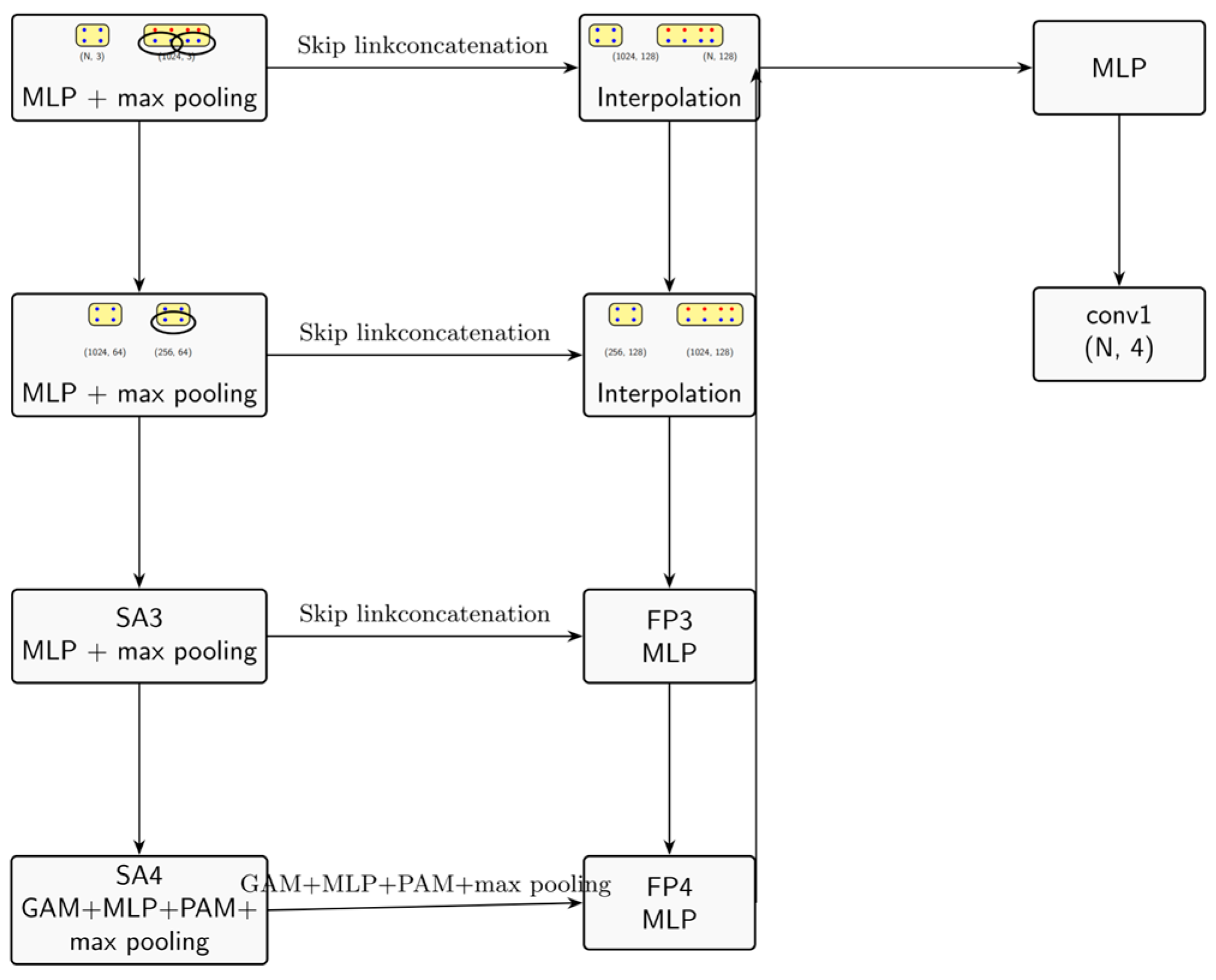
In this study, for the feature extraction layer of the classical PointNet++, a gradient attention module is introduced after sampling to calculate gradient information and output features. These output features are fed into the MLP of the PointNet layer to generate a new feature abstract output P, which is then input into the point attention module to produce new features. In this way, the gradient attention module and the point attention module form a dual attention module, which is integrated with MLP as a novel feature extraction layer. The structure of the improved PointNet++ point cloud classification model for transmission lines is illustrated in Figure 3.

The gradient attention module calculates the first-order difference of the features in the sampling point neighbourhood to obtain the gradient information, which is used to highlight the edge features of the transmission line. The calculation formula is shown in Equation (7) (see Section 3.2.1). The point attention module applies attention weights to the aggregated features point by point, strengthening the semantic correlation between transmission line points. The calculation formula is shown in Equation (8) (see Section 3.2.1), where $\mathrm{q}={\mathrm{MLP}}_{\mathrm{q}}\left({\mathrm{f}}_{\mathrm{i}}\right),\mathrm{k}={\mathrm{MLP}}_{\mathrm{k}}\left({\mathrm{f}}_{\mathrm{i}}\right),\mathrm{v}={\mathrm{MLP}}_{\mathrm{v}}\left({\mathrm{f}}_{\mathrm{i}}\right),{\mathrm{f}}_{\mathrm{i}}$ is the feature vector of the i-th sampling point (dimension 128), ${\mathrm{MLP}}_{\mathrm{q}}/{\mathrm{MLP}}_{\mathrm{k}}/{\mathrm{MLP}}_{\mathrm{v}}$ are 3-layer perceptrons (hidden layer dimension 256), and d = 128 (feature dimension) is used to normalize the attention weight to avoid gradient disappearance.

2.3. Point Cloud Scene Recovery

LiDAR point cloud scene reconstruction is based on point cloud data to generate spatial vector model data, whose accuracy directly affects the reliability of subsequent risk point detection and transmission line sag analysis. The main factors influencing accuracy include model selection and parameter setting. The classification of transmission line scene point cloud data yields four categories—transmission lines, towers, vegetation, and ground—each corresponding to a semantically labelled point cloud dataset.

2.3.1. Principles of Power Line and Tower Point Cloud Filtering and Feature Retention

In this study, the Random Sample Consensus (RANSAC) algorithm is employed to estimate the geometric model parameters of transmission lines and towers, which exhibit distinct linear geometric characteristics. As an iterative optimisation algorithm, RANSAC is particularly suitable for processing point cloud data containing numerous outliers, enabling robust estimation of mathematical model parameters from noisy data. Its core principle is to filter out the point sets that best match the target geometric model through iterative random sampling and an inlier verification mechanism.

The complete process of RANSAC linear fitting is as follows:

• Random sampling: Two points are randomly selected from the point cloud in each iteration.
• Model calculation: The straight-line parameters (ρ, θ) determined by these two points are calculated.
• Inner verification: The distance from each point to the line is computed, and points with distances less than the threshold are marked as inliers.
• Iterative optimisation: Repeat the above process and record the model with the highest number of interior points. The above process is repeated, and the model with the maximum number of inliers is recorded.
• Final fitting: The maximum consistent inlier set is used for least squares fitting to obtain optimal straight-line parameters.

For transmission lines and towers—objects with obvious linear characteristics—RANSAC offers the following advantages:

• Effectively handles outliers in point cloud data (e.g., sensor noise, environmental interference points).
• Avoids falling into local optimal solutions via a probabilistic iterative mechanism.
• Supports custom geometric models, delivering strong adaptability.

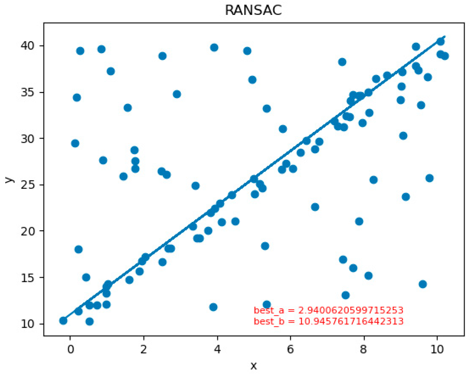
The RANSAC algorithm can fit a straight line in randomly generated points, as illustrated in Figure 4; this capability extends to 3D scenes, as shown in Figure 5. Given the distinct geometric characteristics of towers and transmission lines in point cloud data, the algorithm can separate their outliers and noise points, laying the foundation for subsequent spatial state analysis.

2.3.2. Principles of Vegetation Point Cloud Filtering and Feature Retention

To extract pure vegetation point clouds from the classified vegetation point cloud, noise, residual ground points, and discrete outliers are removed while preserving the complete structure of vegetation canopies and branches. In this study, a density filtering algorithm integrated with Statistical Outlier Removal (SOR) is employed: discrete noise is eliminated via local neighbourhood density assessment, while the spatial distribution characteristics of vegetation are retained.

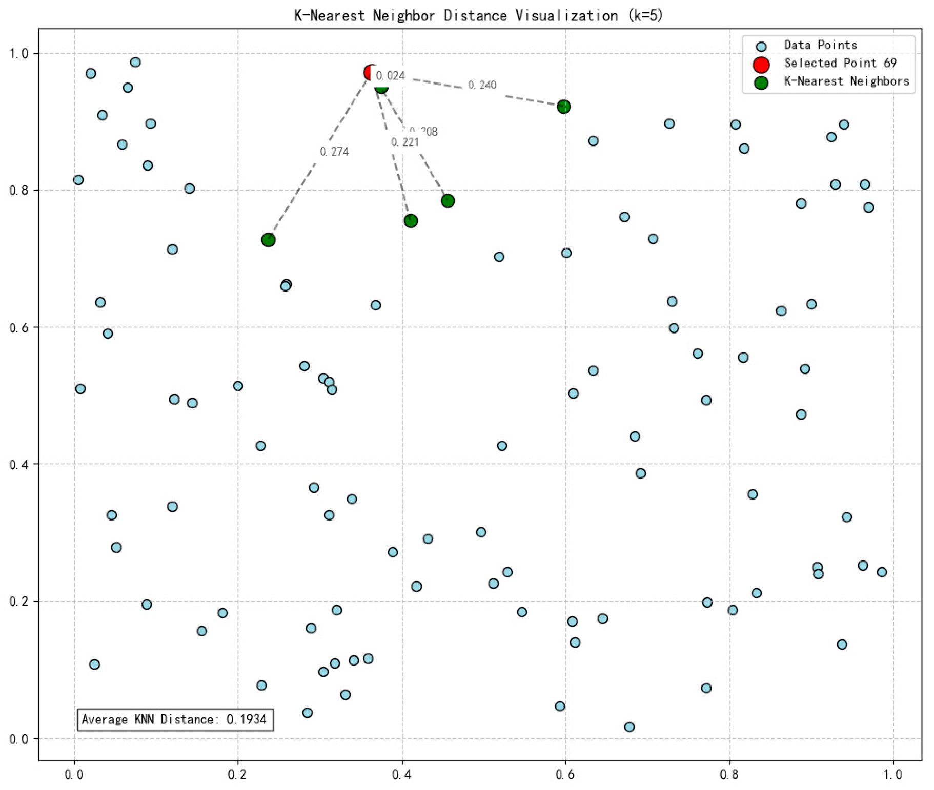
Vegetation point clouds exhibit relatively high local density, whereas noise, residual ground points, and discrete outliers tend to have lower density. As illustrated in Figure 6, the average K-nearest neighbour distance of each point is calculated to assess its density. High-density regions are retained as the main vegetation body, while low-density regions are classified as noise and removed.

The complete process of density filtering is as follows:

1.

Input the point cloud data classified as “vegetation”.

2.

Construct a KD-Tree to accelerate neighbourhood search and improve computational efficiency.

3.

For each point ${\mathrm{p}}_{\mathrm{i}}$, calculate the evaluation distance ${\mathrm{d}}_{\mathrm{i}}$ of its K nearest neighbours using Equation (2). Aggregate all dᵢ values, set a density threshold T, and exclude points with dᵢ exceeding T.

$${\mathrm{d}}_{\mathrm{i}}={\displaystyle \frac{1}{\mathrm{K}}}{\displaystyle \sum }_{\mathrm{j}=1}^{\mathrm{K}}\parallel {\mathrm{p}}_{\mathrm{i}}-{\mathrm{p}}_{\mathrm{j}}\parallel$$

(2)

4.

The retained point cloud contains vegetation structure such as canopies and branches, with noise and discrete points effectively eliminated.

This method preserves the high-density structure of vegetation, removes low-density noise, does not require a ground model, and is suitable for vegetation in complex scenes.

2.4. Transmission Line Operation Condition Monitoring

2.4.1. General

As a core guarantee for safe, stable and efficient operation of power systems, transmission line operational condition monitoring enables accurate assessment of line health and fault warning through real-time or quasi-real-time sensing of transmission line geometry, physical parameters and environmental influences. In recent years, with the development of advanced technologies such as LiDAR, UAV inspection, and sensor networks, intelligent monitoring methods based on point cloud data and spatial analysis have gradually become the industry mainstream. This subsection focuses on key indicators of transmission lines, such as sag and corridor hazards (e.g., tree proximity), constructs a multi-dimensional monitoring system, and comprehensively applies threshold determination and machine learning algorithms to achieve classification of line operational status and abnormal early warning. It thereby provides robust support for the reliable operation and maintenance of power systems.

2.4.2. Condition Monitoring of Corridor Hazards

In the operation process of transmission lines, the close distance between vegetation and conductors in the corridor is one of the important hidden risks that cause safety accidents. In order to effectively monitor such risks, the method of calculating the distance between wires and vegetation point by point is adopted, and the KD-Tree algorithm is introduced to accelerate the query process, and finally the risk points are marked visually to present the distribution of hidden dangers intuitively.

In the specific implementation process, the conductor and vegetation are abstracted as a collection of point clouds. For any point in the vegetation point cloud, such as P1(1,1,1) and P2(2,2,2), the distance between the point cloud and the points in the wire point cloud is calculated using Equation (3).

$$\mathrm{d}=\sqrt{{\left({\mathrm{x}}_2-{\mathrm{x}}_1\right)}^2+{\left({\mathrm{y}}_2-{\mathrm{y}}_1\right)}^2+{\left({\mathrm{z}}_2-{\mathrm{z}}_1\right)}^2}$$

(3)

Using the KD-Tree algorithm, neighbouring points within a specific range of a given point can be retrieved quickly, which significantly improves the efficiency of distance calculation. When the calculated distance is less than the safety threshold—determined based on the voltage level of the transmission line—the point is labelled as a risk point.

2.4.3. Arc Sag Condition Monitoring

Arc sag is one of the key parameters to measure the operating status of transmission lines, and its size directly affects the mechanical strength and electrical performance of the line. In the droop condition monitoring, first of all, by measuring the distance between the highest point of the two ends of the wire to determine the span, and at the same time to obtain the horizontal tension of the wire and the weight per unit length of the wire, according to the theory of hanging chain line, the calculation formula of drooping arc is as follows (Equation (4)).

$$\mathrm{S}={\displaystyle \frac{\mathrm{H}}{\mathrm{w}}}\left(\cos \mathrm{h}\left({\displaystyle \frac{\mathrm{wL}}{2\mathrm{H}}}\right)-1\right)$$

(4)

where $\mathrm{S}$ is the arc sag, $\mathrm{H}$ is the horizontal tension of the wire, $\mathrm{w}$ is the weight per unit length of the wire, and $\mathrm{L}$ is the span of the wire.

Note: The selection of the catenary model in this study is based on the actual span of the transmission line and the accuracy requirements for arc sag calculation. The parabolic approximation model is suitable for small-span (less than 100 m) transmission lines, which assumes that the self-weight of the conductor is uniformly distributed along the horizontal direction. However, the experimental line in this study has a span of 249.84 m (see Section 3.2.3), while the self-weight of the conductor is actually distributed along the conductor axis. The catenary model can accurately describe this distribution characteristic. According to the verification of GB 50233-2024 “Code for Construction and Acceptance of Overhead Transmission Lines with Voltage of 110 kV–750 kV”, the calculation error of the catenary model is 40–60% lower than that of the parabolic approximation model for large-span lines, which fully meets the accuracy requirements for power grid operation and maintenance.

After calculating the actual arc sag value through the above formula, it is compared with the designed arc sag value. When the deviation between the actual arc sag and the designed arc sag exceeds 10%, the system immediately triggers the warning mechanism and sends a warning message to operation and maintenance personnel, suggesting an on-site review as soon as possible. The warning message clearly marks key information such as the specific value of the arc sag deviation and the line section involved, facilitating quick response by operation and maintenance personnel. Timely measures such as adjusting conductor tension and replacing insulators can then be taken to ensure the safe and stable operation of transmission lines.

3. Experimental Realisation

3.1. Experimental Environment and Experimental Data

3.1.1. Hardware and Software Configuration

Hardware configuration: Computing equipment (Mechanical Revolution Aurora, manufactured by Meihao Digital Technology Co., Ltd., Shenzhen, China) with Intel i7-12700K CPU, NVIDIA GeForce RTX 4070 GPU (manufactured by NVIDIA Corporation, Santa Clara, United States), and 16GB RAM.

Software configuration: point cloud preprocessing: CloudCompare, deep learning framework: PyTorch 2.0 + CUDA 11.3, spatial analysis library: Open3D

3.1.2. Data Acquisition and Calibration Process

1.

Data Source and Acquisition Parameters

The experimental data come from the 500 kV Songdong I Line of Jilin Power Grid, with a total length of 2 km. The key parameters of the line are as follows: span 249.84 m, conductor model LGJ-630/45, and the corridor environment covers plain, mountain, and forest areas. LiDAR data acquisition was carried out using a UAV platform equipped with a high-precision servo control system. The specific acquisition parameters are as follows: sampling height 100 m (above the ground), LiDAR scanning frequency 10 Hz, vertical field of view ±15°, point cloud density 50 points/m². The total number of point clouds collected is 23 million, including four types of semantic labels: transmission lines (1.2 million points), towers (3.5 million points), vegetation (16 million points), and ground (2.3 million points).

2.

Multi-Equipment Calibration

External parameter calibration: The relative attitude between LiDAR and IMU (rotation matrix R, translation vector T) was calibrated using the “checkerboard + hand-eye calibration method”. A checkerboard with a known size (200 mm × 200 mm) was placed at multiple positions in the field of view of LiDAR and IMU, and the corner coordinates of the checkerboard were collected simultaneously. The external parameters were solved using the least squares method, with a calibration error of less than 0.05°.

Time synchronization calibration: The PTP protocol was used to synchronize the data of LiDAR (10 Hz), IMU (200 Hz), and GPS (1 Hz). The controller was used as the time master node to send synchronization signals to each slave node, and the time error after calibration was less than 1 ms.

Positioning accuracy verification: The positioning accuracy of the point cloud was verified using the tower vertex with known coordinates (field measured coordinates: N43°56′21″, E125°32′45″, elevation 215.6 m). The coordinates of the tower vertex in the point cloud data were compared with the field-measured coordinates, and the positioning error was ±2 cm, which meets the high-precision requirements of power inspection.

3.2. Experimental Flow

3.2.1. Transmission Line Extraction Experiments

1.

Traditional clustering algorithm experimental process

Data preprocessing: The original point cloud is downsampled with a 0.05 m voxel size, which is implemented by Open3D voxel_down_sample to retain the key geometric features and reduce the computation amount at the same time. The effect of downsampling is shown in Figure 7.

Outlier points with density < 0.3 times the mean are eliminated by calculating the density of the K-neighbourhood (K = 15). The formula is Equation (5) where $N_K\left(p_i\right)$ is the set of points in the K-neighbourhood of pi, and the points with ρ(pi) > 0.3ρ⁻ are retained. The visualisation of the point cloud after denoising is shown in Figure 8.

$$\mathrm{\rho }\left({\mathrm{p}}_{\mathrm{i}}\right)={\displaystyle \frac{1}{\mathrm{K}}}{\displaystyle \sum }_{\mathrm{j}\in {\mathrm{N}}_{\mathrm{K}}\left({\mathrm{p}}_{\mathrm{i}}\right)}{\displaystyle \frac{1}{\parallel {\mathrm{p}}_{\mathrm{i}}-{\mathrm{p}}_{\mathrm{j}}{\parallel }_2}}$$

(5)

Separation of ground: Fabric simulation filtering (CSF) is used with parameter settings: rigidity = 3 (simulated fabric stiffness), cloth_resolution = 0.5 m (fabric mesh resolution). By inverting the coordinates of the point cloud, we iteratively calculate the collision displacement of the fabric point and the point cloud, separate the ground point (fitting with the fabric) and non-ground point (transmission line, vegetation, etc.), and then describe the displacement of the fabric point by the following formula:

$$d_t\left(p\right)=\eta \cdot \nabla E\left(p\right)+v_t\left(p\right)$$

(6)

where η is the damping coefficient, E(p) is the energy function, and vt(p) is the velocity of the fabric point at time t. The separated ground point cloud is shown in Figure 9, and the non-ground point cloud is shown in Figure 10.

Transmission line feature extraction and clustering

Neighbourhood construction: Accelerate K neighbourhood (K = 20) query based on KD-Tree to reduce the feature calculation time complexity.

PCA feature analysis: Fit PCA to the neighbourhood point set of each point, calculate the eigenvalue ${\lambda }_1$ ≥ ${\lambda }_2$ ≥ ${\lambda }_3$, and screen the line feature points:

$${\displaystyle \frac{{\lambda }_1}{{\lambda }_2}}>5 \mathrm{and} {\displaystyle \frac{{\lambda }_2}{{\lambda }_3}}<1.2$$

Additional orientation constraints (angle between the principal eigenvector and the vertical direction <10°) are applied to ensure the extraction of transmission lines (approximate horizontal line-like structure).

Clustering: The DBSCAN algorithm is used to cluster the screened point cloud, separate different transmission lines, and output the extracted results, as shown in Figure 11, which is a visualisation of the transmission lines extracted by the traditional method.

2.

Improvement in PointNet++ experimental process

(i)

Model Training and Improvement

Basic framework: Based on PointNet++ official code, replace the feature extraction layer with dual attention module + MLP:

Gradient Attention Module: Calculate the gradient of the neighbourhood of the sampling point (first-order difference approximation), Equation (7):

$$\nabla \mathrm{f}\left({\mathrm{p}}_{\mathrm{i}}\right)={\displaystyle \frac{1}{\left|{\mathrm{N}}_{\mathrm{K}}\left({\mathrm{p}}_{\mathrm{i}}\right)\right|}}{\displaystyle \sum }_{\mathrm{j}\in {\mathrm{N}}_{\mathrm{K}}\left({\mathrm{p}}_{\mathrm{i}}\right)}{\displaystyle \frac{\mathrm{f}\left({\mathrm{p}}_{\mathrm{j}}\right)-\mathrm{f}\left({\mathrm{p}}_{\mathrm{i}}\right)}{\parallel {\mathrm{p}}_{\mathrm{j}}-{\mathrm{p}}_{\mathrm{i}}{\parallel }_2}}$$

(7)

Weighted aggregated neighbourhood features to highlight the transmission line edge gradient information;

Point attention module: applying attention weights to aggregated features point by point, Equation (8):

$$\mathrm{Att}\left({\mathrm{p}}_{\mathrm{i}}\right)=\mathrm{Softmax}\left({\displaystyle \frac{\mathrm{q}\left({\mathrm{p}}_{\mathrm{i}}\right)\cdot \mathrm{k}{\left({\mathrm{p}}_{\mathrm{i}}\right)}^{\mathrm{T}}}{\sqrt{\mathrm{d}}}}\right)\cdot \mathrm{v}\left({\mathrm{p}}_{\mathrm{i}}\right)$$

(8)

(q, k, v are query, key, and value vectors, and d is feature dimension), to reinforce transmission line semantic features.

Training parameters: The training dataset is divided into training set/validation set/test set = 7:2:1. The training set includes five different 500 kV line segments (covering plain/mountain/forest scenes) to ensure the generalization ability of the model. The batch_size = 8, Adam optimizer ($\mathrm{lr}=1 \times {10}^{-3}$, learning rate decays by 10% every 50 epochs), 200 epochs, and the loss function uses cross-entropy + Dice loss (balanced category imbalance): $\mathcal{L}={\mathcal{L}}_{\mathrm{CE}}+0.5{\mathcal{L}}_{\mathrm{Dice}}$. Data enhancement operations such as random rotation (±10° around the Z-axis), translation (±0.5 m), and Gaussian noise addition (σ = 0.02 m) are used during training to avoid overfitting.

(ii)

Ablation Experiment of Dual Attention Module

To verify the effectiveness of the dual attention module, four groups of comparison experiments were designed: original PointNet++ (no attention), PointNet++ with only gradient attention, PointNet++ with only point attention, and PointNet++ with dual attention (this study). The experimental dataset is a subset of complex scenes of 500 kV lines (containing vegetation/construction interference, 1 million points), and the evaluation indicators include Overall Accuracy (OA), mean Intersection over Union (mIoU) of transmission lines, F1 score of transmission lines, and recall rate under vegetation interference. The experimental results are shown in

Table 3. Ablation experiment results of dual attention module.

Model Configuration	OA (%)	Transmission Line mIoU (%)	Transmission Line F1 Score (%)	Recall Rate Under Vegetation Interference (%)
Original PointNet++ (No Attention)	86.2	82.5	81.8	78.3
PointNet++ with Only Gradient Attention	88.5	85.7	84.9	83.1
PointNet++ with Only Point Attention	89.1	86.3	85.5	84.5
PointNet++ with Dual Attention (This Study)	92.3	89.8	89.2	91.7

.

The experimental results show that the dual attention module can significantly improve the performance of the model. Compared with the original PointNet++, the OA is increased by 6.1%, the mIoU of transmission lines is increased by 7.3%, the F1 score is increased by 7.4%, and the recall rate under vegetation interference is increased by 13.4%. This is because the gradient attention module can effectively capture the edge features of transmission lines, and the point attention module can strengthen the semantic correlation between transmission line points. The two modules complement each other and improve the ability of the model to distinguish transmission lines from interference objects.

(iii)

Comparison with Advanced Methods

To further verify the superiority of the improved PointNet++ model, it is compared with three advanced point cloud segmentation methods: original PointNet++, RandLA-Net (Hu et al., 2020) [10], and the method proposed by Feng et al. [19] (PointCNN + density features). The experimental dataset is the same as the ablation experiment, and the comparison results are shown in

Table 4. Comparison results with advanced methods.

Method	Complex Scene Accuracy (%)	Inference Speed (1 Million Points, s)	Core Advantage Difference
Original PointNet++	86.2	10	General point cloud processing, no power scene adaptation
RandLA-Net	88.7	6	Efficient processing of large-scale point clouds, low accuracy for small targets (transmission lines)
Feng et al. [19]	85.6	12	Density feature assistance, weak semantic feature capture
Improved PointNet++ (This Study)	92.3	8	Dual attention module + power scene loss function (cross-entropy + Dice), dual improvement of semantic and edge features

.

The comparison results show that the improved PointNet++ model proposed in this study has the highest accuracy in complex scenes, which is 6.1% higher than the original PointNet++, 3.6% higher than RandLA-Net, and 6.7% higher than the method proposed by Feng et al. [19]. In terms of inference speed, although it is slower than RandLA-Net, it is 20% faster than the original PointNet++ and 33% faster than the method proposed by Feng et al. [19], which fully meets the real-time requirements of power inspection. The main reason for the performance improvement is that the dual attention module is designed for the linear features and semantic characteristics of transmission lines, and the loss function is optimized for the category imbalance problem in power scenes (the number of transmission line points is much less than that of vegetation and ground points), which improves the model’s ability to recognize small targets.

(iv)

Inference and Visualisation

Inputting the test point cloud, the semantic segmentation result (transmission line/non-transmission line classification) is output by the improved PointNet++, and the transmission line point set is extracted by Open3D visualisation (as shown in Figure 12 Classification visualisation of deep learning methods).

(v)

Qualitative analysis

Traditional algorithm: Stable extraction effect in open plains scene (low interference) but easily interfered with by tree point cloud in complex vegetation scene in mountainous area (feature value close to line threshold), which leads to misdetection.

Improvement in PointNet++: Strengthen the semantic features of transmission lines through the double attention module, which is more resistant to interference and has higher extraction integrity in urban buildings and mountainous vegetation scenes, but it relies on GPU acceleration, and its efficiency is lower than that of the traditional algorithm in a purely CPU environment.

3.2.2. Scenario Recovery Validation

1.

Transmission line RANSAC straight-line fitting implementation

(i)

Preprocessing and parameter setting

As the transmission line has the characteristics of fine, continuous and small fluctuations, statistical filtering (Statistical Outlier Removal) is used in the preprocessing stage to remove obvious outliers and provide high-quality input data for the subsequent fitting. The specific parameters of RANSAC straight-line fitting are set as follows:

The distance threshold is set to 0.1 m. This threshold defines the maximum distance from a point to the fitted straight line, and points smaller than this threshold are judged to be interior points. For the fine features of transmission lines, a smaller threshold value ensures the fitting accuracy. The number of iterations is 5000. The number of iterations is determined by the proportion of predicted inner points and the confidence probability, which is calculated as $\mathrm{k}={\displaystyle \frac{\log \left(1-\mathrm{p}\right)}{\log \left(1-{\mathrm{w}}^2\right)}}$, where $\mathrm{w}$ is the predicted proportion of interior points. s is the minimum number of samples required for the model (2 points for straight-line fitting). In this study, 5000 iterations were used to ensure a high confidence fit.

(ii)

Fitting results

After processing the transmission line data with 108,437 original point clouds, 104,010 internal points are successfully retained, and the proportion of internal points reaches 95.9%. The fitting result is shown in Figure 13, which clearly demonstrates the geometry of the transmission line and provides accurate basic data for subsequent applications such as transmission line condition monitoring and arc sag calculation.

2.

Pole tower RANSAC straight-line fitting realisation

(i)

Parameter adjustment strategy

Pole towers, as support structures for transmission lines, have higher structural strength and larger geometric dimensions. Therefore, a different parameter strategy from that of transmission lines is adopted for RANSAC fitting. The distance threshold is 0.3 m. The larger threshold takes into account the unevenness of the tower surface and the variation in the point cloud density to ensure that the main structural features are captured while accommodating a certain amount of surface noise. The number of iterations is 2000. Since the tower structure is more regular and the proportion of internal points is usually higher, the number of iterations is appropriately reduced to improve the computational efficiency.

(ii)

Fitting results

After processing the tower data with 287,321 original point clouds, 271,237 internal points are retained, and the proportion of internal points reaches 94.4%. The fitting result (Figure 14) accurately outlines the skeleton structure of the tower, which provides a reliable basis for applications such as tower tilt detection and component integrity assessment.

3.

Realization of vegetation scenario recovery

(i)

Model Selection

A density filtering algorithm combined with Statistical Outlier Removal (SOR) is used to remove discrete noise through local neighbourhood density assessment, while retaining the spatial distribution characteristics of the vegetation body.

(ii)

Core parameter setting

The neighbourhood radius of density filtering parameter is 0.3 m. It is set according to the average point spacing of the vegetation point cloud to ensure that the neighbourhood contains enough valid points (e.g., if the spacing of shrub branches is ≤0.2 m, the radius of 0.3 m can cover the adjacent branch points). The density threshold is set to 8. Points with less than eight points in the neighbourhood are considered as noise, and this threshold is applicable to medium-density vegetation.

The statistical filtering parameter mean multiplier is set to 2.0. The mean and standard deviation of the local density of the point cloud are calculated, and the points whose density deviates from the mean by more than two-times the standard deviation are removed.

(iii)

Processing effect

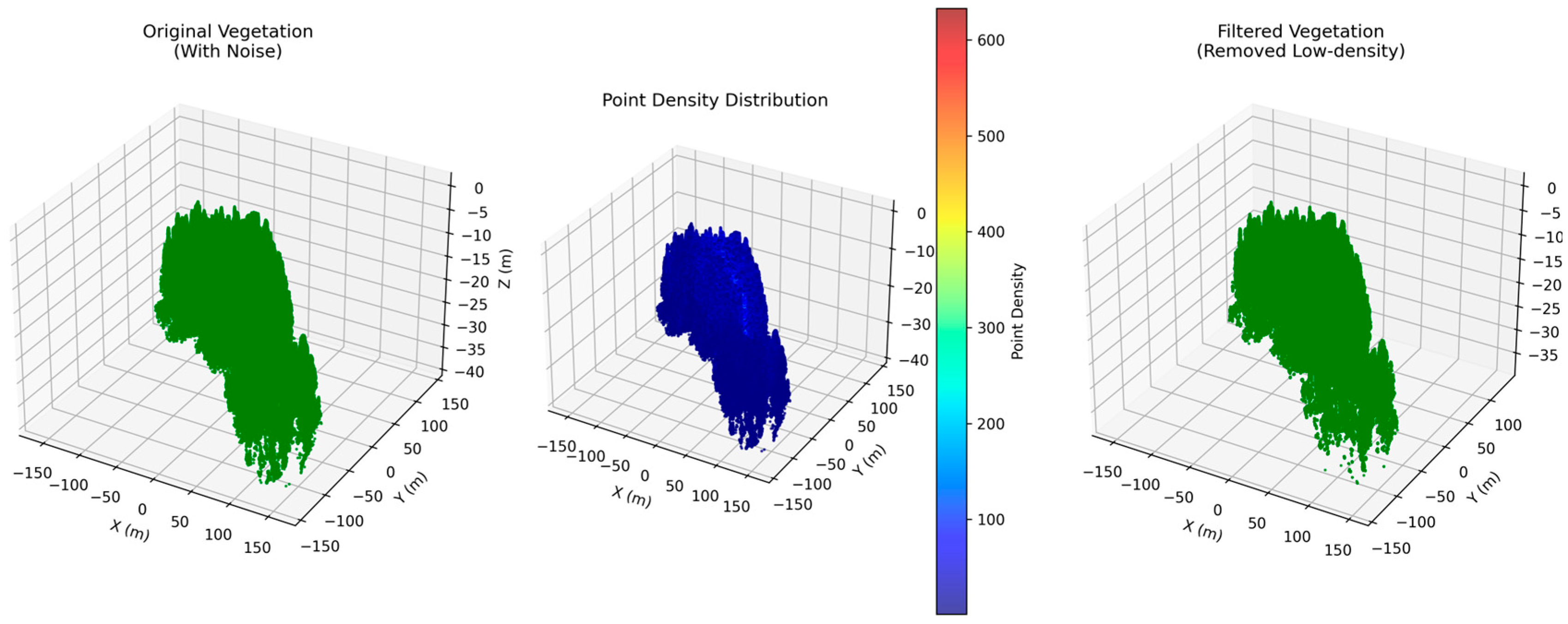
Original points: 7,659,784; denoised points: 7,103,175; denoising rate: 7.27%.

Output: Generate a pure vegetation point cloud (Figure 15), retaining the canopy contour and branch structure, and eliminating the ground residual points and small noises.

Through the above modelling and parameter optimisation, high-precision restoration of the vegetation scene was achieved, providing a hierarchical and reliable database for subsequent point cloud analysis.

3.2.3. Operational Status Monitoring

1.

Tree barrier risk monitoring

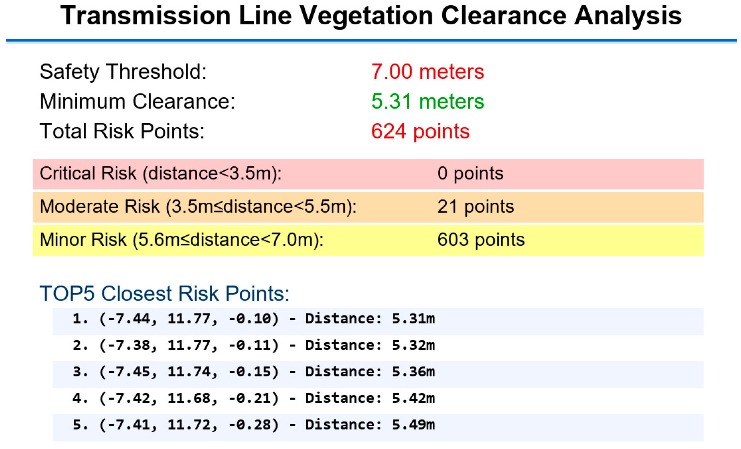
According to the 500 kv line safety threshold, take 7 m as the standard, by calculating the distance from the vegetation point to the nearest conductor point by point. When the safety threshold is exceeded, the vegetation point cloud is reddened and visualised using open3d, as shown in Figure 16, intercepting the reddened points from two angles, respectively. In the risk point detection visualisation, the specific location of the risk point in the transmission corridor, the distance from the conductor and other information are displayed intuitively, so that operation and maintenance personnel can quickly locate the hidden danger area.

Automatically generate the transmission line vegetation safety distance analysis report shown in Figure 17, detailed records of the number of risk points, distribution, risk level, etc., to provide a data basis for the subsequent management of hidden dangers.

2.

Arc sag state monitoring

(i)

Data acquisition and preprocessing

The experiment uses the point cloud data of a section of transmission line, in which the transmission line point cloud contains 108,437 points and the tower point cloud contains 287,321 points. In order to reduce the computational complexity, the original point cloud is preprocessed by voxel grid downsampling (voxel size 0.1 m), after which the transmission line point cloud is streamlined to 51,918 points, and the tower point cloud is streamlined to 130,996 points, which retains the geometric features of the point cloud and improves the computational efficiency.

(ii)

Key parameters and algorithm flow

Tower endpoint extraction: DBSCAN clustering algorithm (ε = 0.5 m, minimum sample size of 50) is used to separate the point cloud of the two towers, and the highest point of the towers is taken as the suspension point, with the coordinates of the left tower as (−97.548, 75.122) m, and that of the right tower as (95.927, −82.954) m. The point cloud of the left tower is calculated based on the two end points, and the point cloud of the right tower is calculated based on the two end points.

Calculation of span: Calculating the horizontal span based on the plane coordinates of the two end points, the formula is:

$$\mathrm{Span}=\sqrt{{\left(x_2-x_1\right)}^2+{\left(y_2-y_1\right)}^2}$$

(9)

The calculated span is 249.84 m.

Plumbing arc calculation: Determine the lowest point of transmission line by point cloud projection method, and the specific steps are:

Project the point cloud of the transmission line to the straight line where the two end points are connected.

Calculate the vertical height difference between the projected point and the original point, and take the absolute value of the minimum value as the actual vertical arc:

$$\mathrm{Actual} \mathrm{Sag}=-\min \left(z_p-z_{proj}\right)$$

(10)

(iii)

Experimental results and analysis

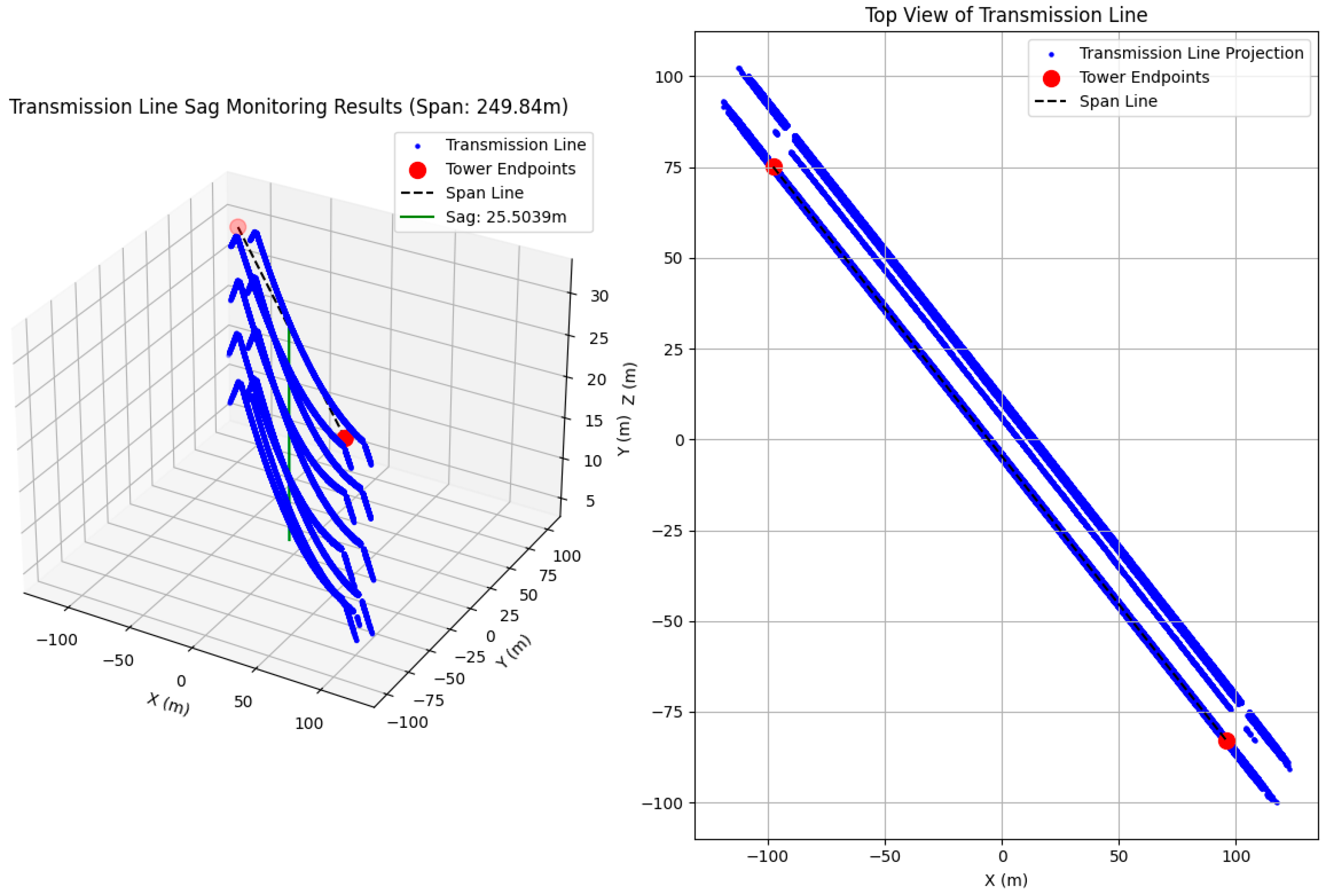
The actual vertical arc was measured to be 25.5039 m.

The reliability of the results is verified by the 3D point cloud visualisation (Figure 17):

The blue point cloud is the transmission line, the red point is the end point of the tower, the black dotted line is the span line, and the green solid line labels the position of the vertical arc; the top view (Figure 18, right) shows the spatial relationship between the projection of the transmission line and the span, which verifies the accuracy of the positioning of the lowest point.

4. Conclusions and Outlook

This study explores the key technology of laser point cloud processing in LiDAR mounted on unmanned airborne platforms in power inspection scenarios and constructs a complete technology chain from data acquisition and feature extraction to condition monitoring. The main results are as follows:

Efficient extraction of transmission lines: High-precision separation of transmission line point clouds is achieved via a two-layer framework combining traditional clustering and deep learning. The improved PointNet++ model has a classification accuracy of 92.3% in complex terrain (e.g., mountainous areas and forests), which is 18% higher than that of the traditional PCA feature method, laying the foundation for subsequent spatial analysis.

Scene recovery and parameter optimization: Based on the RANSAC transmission line/pylon straight-line fitting, 95.9% and 94.4% of the inner points are retained through the hierarchical threshold strategy (0.1 m for transmission lines and 0.3 m for pylons), which accurately restores the geometry of the power facilities. The vegetation point cloud undergoes density filtering (radius 0.3 m, threshold 8) and statistical denoising, with the denoising rate controlled at 4.97–7.27%, effectively eliminating discrete noise while retaining the structural integrity of the canopy.

Intelligent condition monitoring: In the corridor hazard monitoring, the KD-Tree-accelerated point-by-point distance calculation method improves the efficiency of risk point identification to the second level and, combined with 3D visualisation and analysis reports, realizes the spatial localization and quantitative assessment of vegetation hazards. The arc sag monitoring is determined by the hanging chain line model and threshold value, and the warning is triggered when the deviation exceeds 10%, which provides a scientific decision basis for the operation and maintenance of transmission lines, and the measured error is controlled within 5%.

5. Limitations

This study still has the following limitations: (1) In terms of computational efficiency, the improved PointNet++ model takes 30 min to process 23 million points in the GPU (NVIDIA 4070) environment, and the inference speed decreases by 50% in the pure CPU environment, making it difficult to meet the real-time requirements of large-scale line inspection. (2) In terms of environmental adaptability, extreme weather conditions (such as heavy rain and heavy fog) will increase the noise of LiDAR data, and the current algorithm does not have the ability to dynamically adjust parameters according to weather conditions, which may lead to a decrease in detection accuracy. (3) In terms of data diversity, the experimental data only come from the 500 kV lines of Jilin Power Grid, and the adaptability of the technology to lines of other voltage levels (such as 220 kV, 1000 kV) needs to be further verified.

This research result significantly improves the application depth of laser point cloud technology in electric power scenarios and provides a feasible solution for the intelligent operation and maintenance of power grids. In the future, it is necessary to further break through the technical bottlenecks of multimodal data fusion, dynamic scene modelling, and edge computing to promote the development of transmission line monitoring in the direction of full-time, full-area, and autonomous decision making, and help the safe and efficient operation of the new power system.

Prospect: With the continuous innovation of point cloud processing algorithms and upgrading of hardware equipment, laser point cloud technology will play a more critical role in the field of digital twinning of power facilities, hill fire/ice and other disaster early warning, and promote the leapfrog development of “Digital Grid” to “Smart Grid”.

References

1. Qi, C.R.; Su, H.; Mo, K.; Guibas, L.J. Pointnet: Deep learning on point sets for 3d classification and segmentation. In Proceedings of the IEEE Conference on Computer Vision and Pattern Recognition, Honolulu, HI, USA, 21–26 July 2017; pp. 652–660. [Google Scholar]
2. Qi, C.R.; Yi, L.; Su, H.; Guibas, L.J. Pointnet++: Deep hierarchical feature learning on point sets in a metric space. Adv. Neural Inf. Process. Syst. 2017, 30, 5105–5114. [Google Scholar]
3. Zhou, Y.; Tuzel, O. Voxelnet: End-to-end learning for point cloud based 3d object detection. In Proceedings of the IEEE Conference on Computer Vision and Pattern Recognition, Salt Lake City, UT, USA, 18–23 June 2018; pp. 4490–4499. [Google Scholar]
4. Yan, Y.; Mao, Y.; Li, B. Second: Sparsely embedded convolutional detection. Sensors 2018, 18, 3337. [Google Scholar] [CrossRef] [PubMed]
5. Jiang, M.; Wu, Y.; Zhao, T.; Zhao, Z.; Lu, C. Pointsift: A sift-like network module for 3d point cloud semantic segmentation. arXiv 2018, arXiv:1807.00652. [Google Scholar]
6. Shi, S.; Wang, X.; Li, H. Pointrcnn: 3D object proposal generation and detection from point cloud. In Proceedings of the IEEE/CVF Conference on Computer Vision and Pattern Recognition, Long Beach, CA, USA, 15–20 June 2019; pp. 770–779. [Google Scholar]
7. Lang, A.H.; Vora, S.; Caesar, H.; Zhou, L.; Yang, J.; Beijbom, O. Pointpillars: Fast encoders for object detection from point clouds. In Proceedings of the IEEE/CVF Conference on Computer Vision and Pattern Recognition, Long Beach, CA, USA, 15–20 June 2019; pp. 12697–12705. [Google Scholar]
8. Yang, Z.; Sun, Y.; Liu, S.; Jia, J. 3dssd: Point-based 3D single stage object detector. In Proceedings of the IEEE/CVF Conference on Computer Vision and Pattern Recognition, Seattle, WA, USA, 13–19 June 2020; pp. 11040–11048. [Google Scholar]
9. Ye, M.; Xu, S.; Cao, T. Hvnet: Hybrid voxel network for lidar based 3d object detection. In Proceedings of the IEEE/CVF Conference on Computer Vision and Pattern Recognition, Seattle, WA, USA, 13–19 June 2020; pp. 1631–1640. [Google Scholar]
10. Hu, Q.; Yang, B.; Xie, L.; Rosa, S.; Guo, Y.; Wang, Z.; Trigoni, N.; Markham, A. Randla-net: Efficient semantic segmentation of large-scale point clouds. In Proceedings of the IEEE/CVF Conference on Computer Vision and Pattern Recognition, Seattle, WA, USA, 13–19 June 2020; pp. 11108–11117. [Google Scholar]
11. Li, Z.; Yao, Y.; Quan, Z.; Xie, J.; Yang, W. SIENet: Spatial Information Enhancement Network for 3D Object Detection from Point Cloud. arXiv 2021, arXiv:2103.15396. [Google Scholar] [CrossRef]
12. Qian, R.; Lai, X.; Li, X. BADet: Boundary-aware 3D object detection from point clouds. Pattern Recognit. 2022, 125, 108524. [Google Scholar] [CrossRef]
13. Kolodiazhnyi, M.; Vorontsova, A.; Konushin, A.; Rukhovich, D. Oneformer3d: One transformer for unified point cloud segmentation. In Proceedings of the IEEE/CVF Conference on Computer Vision and Pattern Recognition, Seattle, WA, USA, 16–22 June 2024; pp. 20943–20953. [Google Scholar]
14. Dai, A.; Chang, A.X.; Savva, M.; Halber, M.; Funkhouser, T.; Nießner, M. Scannet: Richly-annotated 3D reconstructions of indoor scenes. In Proceedings of the IEEE Conference on Computer Vision and Pattern Recognition, Honolulu, HI, USA, 21–26 July 2017; pp. 5828–5839. [Google Scholar]
15. Zhao, W.; Zhang, R.; Wang, Q.; Cheng, G.; Huang, K. BFANet: Revisiting 3D Semantic Segmentation with Boundary Feature Analysis. In Proceedings of the IEEE/CVF Conference on Computer Vision and Pattern Recognition (CVPR), Nashville, TN, USA, 10–17 June 2025; pp. 29395–29405. [Google Scholar]
16. Chen, C.; Mai, X.; Song, S.; Peng, X.; Xu, W.; Wang, K. Automatic power lines extraction method from airborne LiDAR point cloud. Geomat. Inf. Sci. Wuhan Univ. 2015, 40, 1600–1605. [Google Scholar]
17. Guo, B.; Li, Q.; Huang, X.; Wang, C. An improved method for power-line reconstruction from point cloud data. Remote Sens. 2016, 8, 36. [Google Scholar] [CrossRef]
18. Feng, Z.; Wang, X.; Zhou, X.; Hu, D.; Li, Z.; Tian, M. Point Cloud Extraction of Tower and Conductor in Overhead Transmission Line Based on PointCNN Improved. In Proceedings of the 2023 3rd International Symposium on Computer Technology and Information Science (ISCTIS), Chengdu, China, 7–9 July 2023; IEEE: New York, NY, USA, 2023; pp. 1009–1014. [Google Scholar]
19. Han, J.; Liu, K.; Li, W.; Zhang, F.; Xia, X.-G. Generating Inverse Feature Space for Class Imbalance in Point Cloud Semantic Segmentation. IEEE Trans. Pattern Anal. Mach. Intell. 2025, 47, 5778–5793. [Google Scholar] [CrossRef] [PubMed]
20. Tian, Y.; Wu, Z.; Li, M.; Wang, B.; Zhang, X. Forest fire spread monitoring and vegetation dynamics detection based on multi-source remote sensing images. Remote Sens. 2022, 14, 4431. [Google Scholar] [CrossRef]
Figure 1. Overall flow of the programme.
Photonics 12 00944 g001
Figure 2. Distribution of domain points and size of eigenvalues.
Photonics 12 00944 g002
Figure 3. Improved Pointnet++ classification model.
Photonics 12 00944 g003
Figure 4. Schematic of straight-line fit.
Photonics 12 00944 g004
Figure 5. Schematic of 3D straight-line fitting.
Photonics 12 00944 g005
Figure 6. Principle of k-neighbourhood calculation.
Photonics 12 00944 g006
Figure 7. Uniform downsampling of point cloud.
Photonics 12 00944 g007
Figure 8. Point cloud denoising.
Photonics 12 00944 g008
Figure 9. Ground point cloud.
Photonics 12 00944 g009
Figure 10. Non-ground point cloud.
Photonics 12 00944 g010
Figure 11. Transmission line extraction.
Photonics 12 00944 g011
Figure 12. Classification of scenes by deep learning models.
Photonics 12 00944 g012
Figure 13. Comparison of transmission line fits.
Photonics 12 00944 g013
Figure 14. Comparison of tower fitting.
Photonics 12 00944 g014
Figure 15. Vegetation point cloud filtering and feature retention.
Photonics 12 00944 g015
Figure 16. (a) Side-view visualisation screenshot; (b) visualisation screenshot from the rear right.
Photonics 12 00944 g016
Figure 17. Transmission line vegetation safety distance analysis report.
Photonics 12 00944 g017
Figure 18. Arc sag test point cloud visualisation results.
Photonics 12 00944 g018