On the Feasibility of Localizing Transformer Winding Deformations Using Optical Sensing and Machine Learning

Abstract

Mechanical vibrations induced by electromagnetic forces during transformer operation can lead to winding deformation or failure, an issue responsible for over 12% of all transformer faults. While previous studies have predominantly relied on accelerometers for vibration monitoring, this study explores the use of an optical sensor for real-time vibration measurement in a dry-type transformer. Experiments were conducted using a custom-designed single-phase transformer model specifically developed for laboratory testing. This experimental setup offers a unique advantage: it allows for the interchangeable simulation of healthy and deformed winding sections without causing permanent damage, enabling controlled and repeatable testing scenarios. The transformer’s secondary winding was short-circuited, and three levels of current (low, intermediate, and high) were applied to simulate varying stress conditions. Vibration displacement data were collected under load to assess mechanical responses. The primary goal was to classify this vibration data to localize potential winding deformation faults. Five supervised learning algorithms were evaluated: Random Forest, Support Vector Machine, K-Nearest Neighbors, Logistic Regression, and Decision Tree classifiers. Hyperparameter tuning was applied, and a comparative analysis among the top four models yielded average prediction accuracies of approximately 60%. These results, achieved under controlled laboratory conditions, highlight the promise of this approach for further development and future real-world applications. Overall, the combination of optical sensing and machine learning classification offers a promising pathway for proactive monitoring and localization of winding deformations, supporting early fault detection and enhanced reliability in power transformers.

1. Introduction

Power transformer windings are critical active components designed to withstand mechanical, thermal, and electrical stresses [1]. Despite their robustness, studies have shown that 12–15% of transformer failures originate from winding-related issues [2]. While this percentage may seem modest, a single failure can cause extensive damage and often results in complete transformer shutdown. Given the essential role and high cost of power transformers in modern power systems, ensuring the structural integrity of their windings is a priority, one that has driven significant research efforts in condition monitoring and fault detection [3,4,5].

Several diagnostic techniques have been developed to monitor transformer health, including vibration-based methods that measure tank or core oscillations [6,7,8]. More recently, frequency response analysis (FRA) has gained traction as a reliable tool for detecting winding displacements and deformation.

In our previous investigation, we demonstrated the advantages of using an optical sensor placed between windings for monitoring vibration signatures associated with structural integrity [9]. Optical sensors offer a distinct advantage in this context due to their immunity to electromagnetic interference [10]. To eliminate external disturbances, a custom open-core transformer was used, isolating the windings for more accurate measurement [11].

Despite these advances, one of the primary challenges that remains is the accurate, real-time localization of winding deformation. In this study, we address this challenge by attaching an optical sensor directly to the winding structure. Vibration signals are collected under multiple mechanical stress scenarios and processed using advanced machine learning algorithms. The goal is to not only detect but also localize winding deformations, laying the groundwork for more intelligent and responsive transformer monitoring systems.

The remainder of this paper is organized as follows: Section 2 recalls some background information on optical fiber Bragg Grating. Section 3 presents the experimental setup, including the custom-designed transformer model, sensor placement, and test scenarios. In Section 4, the machine learning models are introduced, along with their hyperparameter tuning strategies. A comparative analysis of the classification results and a discussion of the implications of the findings are also provided. Finally, Section 5 concludes the paper with key takeaways and directions for future research.

2. Background

Real-time monitoring of power transformer accessories is essential for ensuring the transformer’s reliability and maintaining uninterrupted service [12]. The condition monitoring of power transformer windings has drawn considerable attention from researchers. Frequency Response Analysis, whether performed offline or online, is a well-established and widely recognized technique for detecting mechanical displacements, deformations, and structural damage [13,14]. Mechanical vibrations in transformer windings are primarily caused by electrodynamic forces. These vibrations follow the behavior of a classic mass-spring-damper system. The dynamic behavior of the winding can be described by the equation of motion [9] in Equation (1).

$$m{\displaystyle \frac{d^{2}x}{{dt}^2}}+c{\displaystyle \frac{dx}{dt}}+kx=F\left(t\right)$$

(1)

In this equation, m represents the mass of the winding, c is the damping coefficient, k denotes the mechanical stiffness in newtons per meter (N/m), and $F\left(t\right)$ is the time-dependent electrodynamic force. This force is generally proportional to the square of the current, expressed as Equation (2).

$$F\left(t\right)\alpha I^2$$

(2)

Taking the Fourier transform of Equation (1) leads to the frequency-domain transfer function of the windings’ acceleration response to the applied force. This function, represented by $H\left(j\omega \right)$, is expressed as Equation (3) [7,9]:

$$H\left(j\omega \right)={\displaystyle \frac{\ddot{x}\left(j\omega \right)}{F\left(j\omega \right)}}={\left(M-j{\displaystyle \frac{1}{\omega }}C-{\displaystyle \frac{1}{{\omega }^2}}K\right)}^{-1}$$

(3)

Optical sensors, particularly fiber Bragg Grating (FBG) sensors, have been explored in prior studies as suitable tools for capturing these vibration-induced effects [15]. FBG sensors work based on the principle of Bragg reflection, where the Bragg wavelength, denoted by ${\lambda }_B$ is defined by the relation in Equation (4) [9].

$${\lambda }_B=2n_{eff}\mathsf{\Lambda }$$

(4)

Here, $n_{eff}$ is the effective refractive index of the fiber, and $\mathsf{\Lambda }$ is the spatial period of the Bragg grating embedded within the optical fiber.

In this paper, the used vibration sensor consists of two FBGs inscribed on a single-mode photosensitive fiber using deep-UV phase-mask technology. Each grating has a length of 10 mm with reflectivity of 80%, and the two gratings are separated by a short cavity of 15 mm that forms an interferometric vibration sensor. When strain $\epsilon$ is applied along the fiber, both $n_{eff}$ and $\mathsf{\Lambda }$ change, producing a wavelength shift [9]:

$${\displaystyle \frac{{∆\lambda }_B}{{\lambda }_B}}=\left(1-P_e\right)\epsilon +(\alpha +\xi )∆T$$

(5)

where ${∆\lambda }_B$ is Bragg wavelength shift (pm), $\epsilon$ is axial strain applied to the FBG (µε), $P_e$ introduces effective photo-elastic coefficient of the fiber (≈0.22 for silica), $\alpha$ is known as thermal expansion coefficient of the fiber, $\xi$ is the thermo-optic coefficient of silica fiber, and $∆T$ represents temperature change (°C). In our experiments, temperature effects were negligible or compensated, so the key relation (FBG strain–wavelength sensitivity law) reduces, as shown in Equation (6) [9]:

$${∆\lambda }_B/{\lambda }_B=(1-P_e)\epsilon$$

(6)

The central Bragg wavelength of the gratings was 1550 nm, chosen for compatibility with standard telecommunication interrogators. The sensor was recoated using a Furukawa S541A (Furukawa Electric Corp., Tokyo, Japan) acrylate recoated to provide mechanical robustness and thermal stability up to 150 °C. The packaged sensor (2 mm thickness) was specifically designed to fit inside winding spacers without bonding for repeatable installation and hard contact with winding sections. When the transformer windings experience vibrations, dynamic mechanical stresses are transmitted to the nearby or attached FBG sensor. These stresses lead to two key effects.

• First, they alter the grating period $\mathsf{\Lambda }$ due to mechanical elongation or compression of the fiber.
• Second, they modify the effective refractive index $n_{eff}$ through the photoelastic effect.

Both changes contribute to a measurable shift in the Bragg wavelength ${\lambda }_B$, allowing the FBG sensor to detect and quantify winding vibrations in real time.

3. Experimental Setup

The experimental setup consists of three essential components: a high current source, a test transformer, and an optical sensor connected to its corresponding reading unit. These elements work together to simulate operational conditions and capture the resulting mechanical responses within the transformer windings. As shown in Figure 1, part (a) presents the complete experimental setup, while part (b) displays the physical laboratory model used for the tests. The arrangement allows accurate reproduction of electrical and mechanical stresses and enables real-time monitoring of vibration responses through the optical sensing system.

The FBG sensor was interrogated using a Distributed Feedback (DFB) laser scanner, which continuously sweeps around the Bragg wavelength and detects shifts caused by strain or vibration. The scanner output was transferred to a computer and processed using firmware developed in LabVIEW (v2025 Q3). The acquired signals were transformed into the frequency domain using FFT, and the amplitude at 120 Hz was extracted as the displacement indicator. Prior to transformer tests, the system was calibrated with a YE5503 shaker (Global sensor technology (GST), Manchester, UK) to ensure accurate conversion between wavelength shifts and vibration displacements.

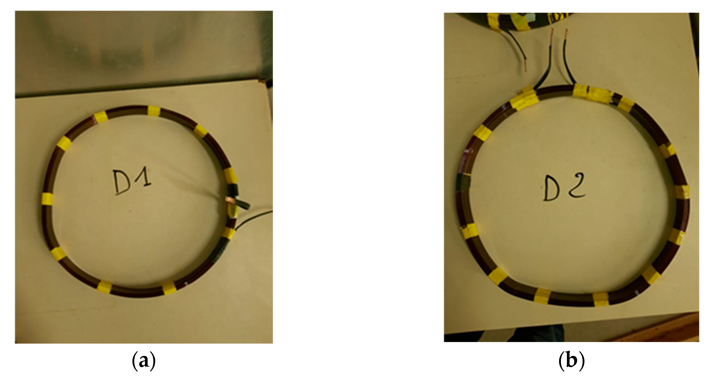
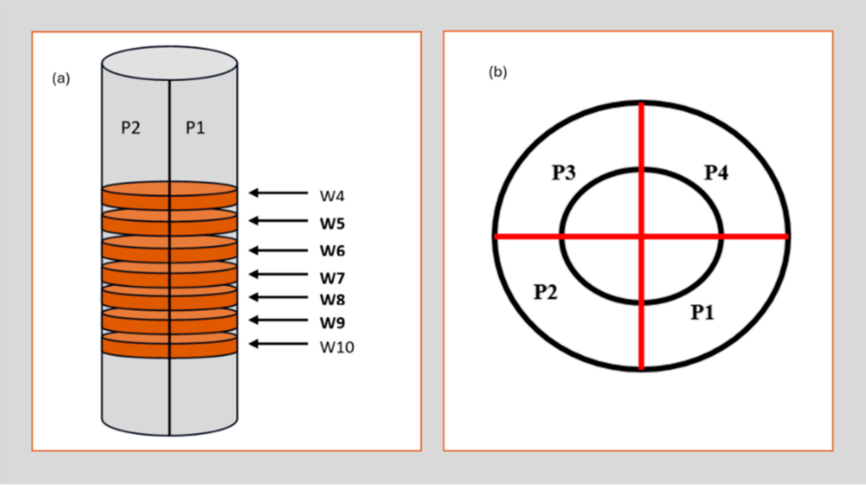
The laboratory dry-type transformer used in this experiment was previously described in earlier investigations and applied current details [9]. Its high-voltage (HV) windings are composed of 16 blocks, numbered 0 to 15, and are divided into four sections: P1, P2, P3, and P4. The optical sensor was mounted on windings W4, W5, W6, W7, W8, W9, and W10. It should be noted that the sensor was positioned on 4 sections of each winding and on each section 5 tests were carried out, so the average of 20 tests makes it possible to obtain the vibration amplitude of a winding in a precise configuration (Figure 2).

The connection between the windings and the current source is in section P4 to minimize the equivalent impedance. The secondary winding of the test transformer is short-circuited, causing the voltage across the secondary to drop to nearly zero. Consequently, the short-circuit current becomes significantly high. This current generates a substantial magnetic flux in the transformer’s magnetic circuit. The reactive component of the short-circuit current, being in phase opposition to the voltage, produces a magnetic field that counteracts the initial magnetic field generated by the primary current. This opposing magnetic field reduces the transformer’s apparent inductance, thereby decreasing its apparent impedance. The high-current source used in the setup is a transformer connected to a 600 V AC supply, with its secondary winding short-circuited. Its output impedance is 0.0016 ohms. To ensure sufficient current for inducing winding vibrations, the impedance of the laboratory transformer windings connected to the high-current source must remain low. The experimental setup includes the dry-type transformer, the high-current source, and a thermal camera housed within a thermal chamber. Outside the chamber, a computer and an ammeter are used to monitor and analyze the experimental data.

To distinguish between different test cases during the experiments, each configuration of the windings and sensor placement was labeled systematically. These labels help track which windings were replaced by deformed ones and where the sensor was positioned during measurement. The configurations are denoted by the prefixes E (for winding arrangements) and Y (for sensor positions).

Table 1. Description of winding and sensor configurations.

Label	Description
E0	Baseline configuration with all windings in healthy condition.
E1	Deformed winding D1 (shown in Figure 2a) replaces winding 7.
E2	Deformed winding D1 replaces winding 6.
E3	Deformed winding D2 (shown in Figure 2b) replaces winding 7.
E4	Deformed winding D2 replaces winding 6.
E5	Combined case: D1 replaces winding 7 and D2 replaces winding 6.
Y0	Sensor placed in a position with only healthy windings nearby.
Y1	Sensor positioned above the deformed winding.
Y2	Sensor placed directly on the deformed winding.
Y3	Sensor located beneath the deformed winding.

and Figure 3 provide a detailed description of each designation used throughout the study [9].

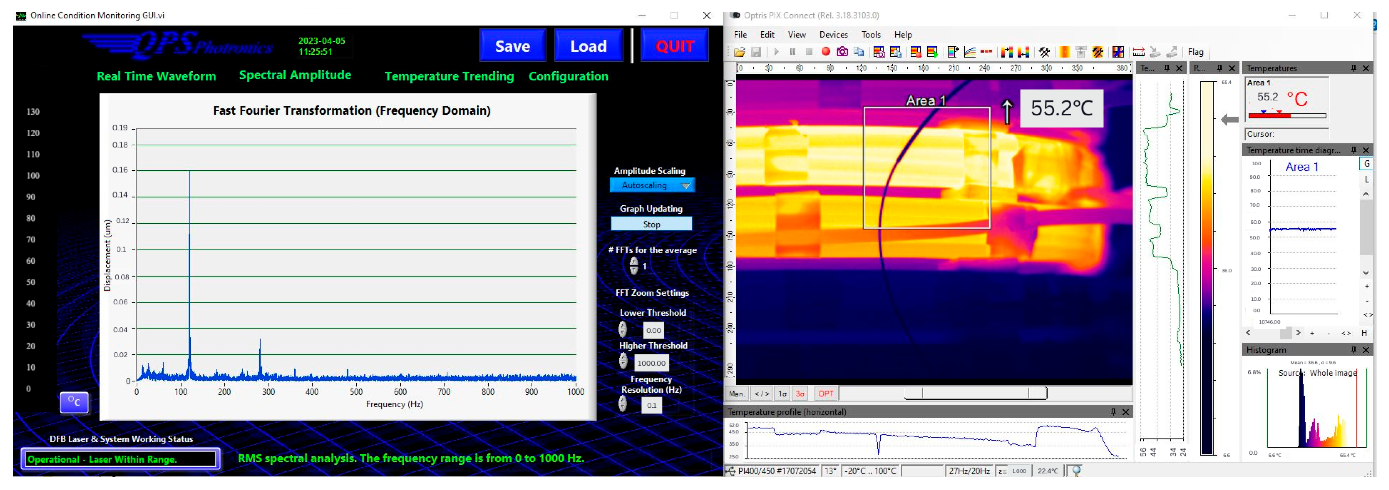
The data acquired during the tests are real-time winding vibration values that the acquisition system processes using the fast Fourier transform. The vibration values are given as a function of the vibration frequency. Figure 4 presents the frequency-domain data alongside the temperature distribution within the windings. The dominant vibration occurs at 120 Hz, which corresponds to twice the 60 Hz power network frequency. This arises because the mechanical forces in the transformer, generated by magnetostriction in the core and electromagnetic forces in the windings, are proportional to the square of the magnetic flux. Squaring a 60 Hz sinusoidal signal produces a component at 120 Hz, explaining why the fundamental vibration appears at this frequency. The amplitudes at 120 Hz are extracted for further analysis to assess the winding dynamics under the measured operating conditions.

4. Results and Discussion

The dataset is structured such that the features correspond to the vibration values measured for each winding (denoted as W4, W5, W6, W7, W8, W9, and W10, where W represents the winding number). The values represent displacement amplitudes (in micrometers, µm) extracted at the fundamental frequency of 120 Hz after FFT processing. The targets are defined as the operational condition of the windings (State) together with the associated severity level (Level). An excerpt of the dataset is presented in

Table 2. Example of dataset structure showing vibration values of windings.

W4	W5	W6	W7	W8	W9	W10	State	Level
0.011977	0.013817	0.015033	0.012935	0.012913	0.014535	0.00983	not fault	Inception Level
0.02252	0.117813	0.0773	0.029075	0.055796	0.048191	0.034295	not fault	Low Level
0.043571	0.171763	0.127405	0.063454	0.095052	0.088966	0.10209	not fault	Intermediate Level
0.12922	0.441948	0.380467	0.194187	0.157496	0.247308	0.155581	not fault	High Level
0.014252	0.066579	0.019945	0.013097	0.015708	0.013601	0.008977	W5 and W6	Inception Level

.

We evaluated five supervised classifiers (Logistic Regression, Linear SVM, K-Nearest Neighbors, Random Forest, and Decision Tree) on FBG-derived vibration displacement measured at seven sensor locations (W4–W10) across five winding configurations (E0–E4) and four current levels. Each measurement record comprises four winding sections (P1–P4); for analysis we adopt a per-part unit (each section as an independent sample described by its mean and standard deviation and the operating context). Model performance is reported using precision, recall, and the F1-score—precision is the proportion of correct positive predictions among all positives; recall (sensitivity) is the proportion of true positives that are correctly identified; F1 balances precision and recall (values near one indicate strong performance, values near zero indicate poor performance). To ensure rigor and comparability, all scores are averaged over a stratified five-fold outer cross-validation. In addition to per-class tables, we summarized overall macro-F1 and balanced accuracy. For each algorithm we present results without improved hyperparameters (defaults) and with improved hyperparameters selected by an inner three-fold grid search that maximizes macro-F1; the corresponding hyperparameter grids are listed in

Table 3. Hyperparameter grids used for model selection (inner three-fold grid; score = macro-F1).

Classifier	Hyperparameter Grid (Candidate Values)
Logistic Regression	$C\in \{0,2,10\}$
Linear SVM	$C\in \{0,\mathrm{2,10}\}$
K-NN	$\mathrm{Neighbors}K\in \{3,5,7,9\}$$;\mathrm{weights}\in \{$$\mathrm{uniform},\mathrm{distance}\}$
Random Forest	$\mathrm{Max}\mathrm{depth}\in \{3,5,7\}$$;\mathrm{Min}\mathrm{samples}\mathrm{per}\mathrm{leaf}\in \{1,2,4\}$
Decision Tree	$\mathrm{Criterion}\in \{$$\mathrm{Gini},\mathrm{entropy},\log \text{-}\mathrm{loss}\}$$;\mathrm{Max}\mathrm{depth}\in \{3,5,7\}$$;\mathrm{Min}\mathrm{samples}\mathrm{per}\mathrm{leaf}\in \{1,2,4\}$

, and representative confusion matrices (without vs. with improvement) are provided for each model.

4.1. Random Forest Classifier

The Random Forest classifier was tested for its ability to distinguish different sensor positions relative to deformed windings using frequency and vibration features. This algorithm, known for its robustness and ensemble learning structure, was evaluated both before and after parameter tuning.

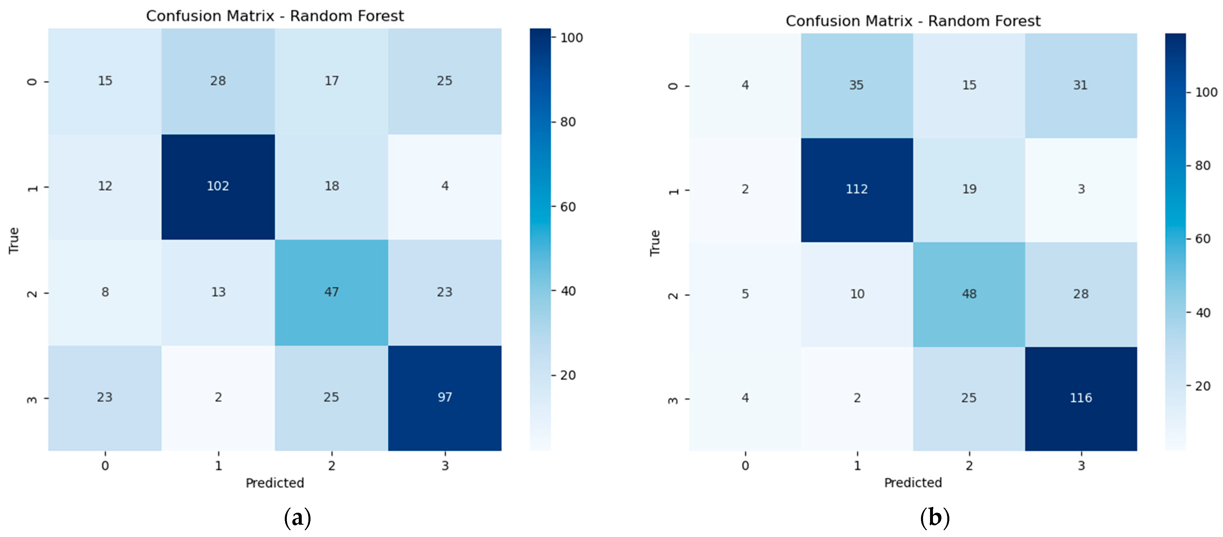
As shown in Figure 5, the confusion matrices highlight the performance differences with and without hyperparameter improvement.

Table 4. Parameters table of Random Forest classifier without improved parameters.

Y	Precision	Recall	F1-Score
0	0.26	0.18	0.21
1	0.70	0.75	0.73
2	0.44	0.52	0.47
3	0.65	0.66	0.66

presents the classification metrics without optimization, while

Table 5. Parameters table of Random Forest classifier with improved parameters.

Y	Precision	Recall	F1-Score
0	0.27	0.05	0.08
1	0.70	0.82	0.76
2	0.45	0.53	0.48
3	0.65	0.79	0.71

includes results after tuning. In both cases, the model performed well for sensor positions Y1 and Y3, achieving a precision of 70% and 65%, respectively, in the untuned model, and maintaining similar performance after tuning.

However, the classifier struggled with Y0 and Y2. In the untuned case, Y0 had a precision of only 26%, and this dropped further to 27% after tuning. For Y2, the F1-score remained low across both setups, indicating difficulty in distinguishing when the sensor was directly on the deformed winding.

Overall, while the Random Forest algorithm demonstrated moderate success in identifying deformation when the sensor was placed above or below the fault (Y1 and Y3), its reliability significantly decreased for other positions, as reflected in both the tables and confusion matrices.

4.2. Support Vector Classifier

The Support Vector classifier was used in this study to classify different winding conditions based on features extracted from frequency response and vibration data, including signals captured by the FBG sensor. The model learns to separate healthy and deformed cases by identifying decision boundaries in the feature space.

Figure 6 illustrates the classification performance visually, while

Table 6. Parameters table of Support Vector classifier without improved parameters.

Y	Precision	Recall	F1-Score
0	0.32	0.08	0.13
1	0.70	0.85	0.76
2	0.49	0.48	0.49
3	0.67	0.83	0.74

The precision is 70% for Y1 and 65% for Y3, indicating that the model shows promise in accurately localizing deformation.

and

Table 7. Parameters table of Support Vector classifier with improved parameters.

Y	Precision	Recall	F1-Score
0	0.27	0.05	0.08
1	0.70	0.82	0.76
2	0.45	0.53	0.48
3	0.65	0.79	0.71

compare the model’s results before and after parameter optimization. The results show that the classifier performs well when the sensor is placed directly above or under the deformed winding, with noticeable improvements in precision and F1-score in those cases. Parameter tuning led to only slight variations overall and suggests that sensor placement has a more significant impact on classification accuracy than hyperparameter adjustment.

4.3. K-Nearest Neighbors Classifier

The K-Nearest Neighbors (KNN) algorithm was also tested to classify winding conditions based on sensor positioning. This method classifies data points by evaluating their similarity to nearby examples in the training set and tries to make it straightforward yet effective for certain types of patterns.

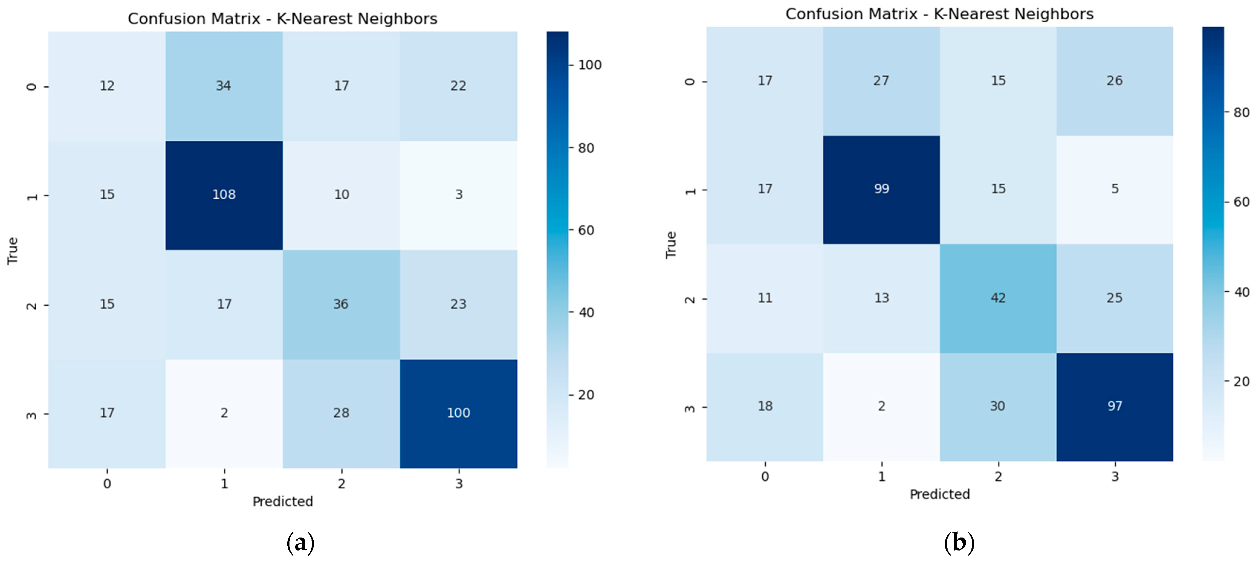
According to the confusion matrices in Figure 7, the classification behavior remained largely unchanged before and after hyperparameter adjustment. As reflected in

Table 8. Parameters table of K-Nearest Neighbors classifier without improved parameters.

Y	Precision	Recall	F1-Score
0	0.27	0.20	0.23
1	0.70	0.73	0.71
2	0.41	0.46	0.44
3	0.63	0.66	0.65

and

Table 9. Parameters table of K-Nearest Neighbors classifier with improved parameters.

Y	Precision	Recall	F1-Score
0	0.27	0.20	0.23
1	0.70	0.73	0.71
2	0.41	0.46	0.44
3	0.63	0.66	0.65

, the classifier consistently produced the strongest results for Y1 and Y3. In both configurations, the precision for Y1 reached 70%, while Y3 held steady around 63–65%, showing that the algorithm reliably identifies deformation when the sensor is positioned above or below the fault.

In contrast, the performance for Y0 and Y2 was considerably weaker, with lower F1-scores and little improvement after parameter tuning. This suggests the KNN model had difficulty capturing the signal characteristics when the sensor was placed on or away from the affected winding without distinct neighboring patterns to guide classification.

Although KNN demonstrated consistent accuracy in some cases, its sensitivity to sensor placement and limited gains from parameter refinement highlight its dependency on data distribution rather than model complexity.

4.4. Logistic Regression

Logistic Regression was tested to classify sensor positions based on frequency and vibration signals collected during the experiment. This linear algorithm predicts class labels by estimating probabilities from the weighted input features.

Figure 8 shows the confusion matrices under two conditions: part (a) illustrates the default model, and part (b) shows the output after parameter adjustment.

Table 10. Parameters table of Logistic Regression classifier without improved parameters.

Y	Precision	Recall	F1-Score
0	0.32	0.16	0.22
1	0.68	0.79	0.73
2	0.53	0.37	0.44
3	0.66	0.86	0.75

and

Table 11. Parameters table of Logistic Regression classifier with improved parameters.

Y	Precision	Recall	F1-Score
0	0.35	0.16	0.22
1	0.67	0.82	0.74
2	0.52	0.35	0.42
3	0.66	0.86	0.75

report the related classification metrics.

The model responded well when the sensor was above or under the deformed winding. Precision reached 68% for Y1 and 66% for Y3 in the initial case, and performance remained steady after tuning. On the other hand, the classifier struggled to identify patterns for Y0 and Y2, where the scores remained low.

Although this model uses a simple structure, it shows consistent behavior for specific sensor locations. Its performance suggests it could be a reliable choice when fast, lightweight fault detection is needed, and sensor placement is favorable.

4.5. Decision Tree

The Decision Tree classifier was evaluated to detect sensor position relative to deformed windings using extracted features from experimental data. This model operates by splitting the data into branches based on conditions that best separate the classes.

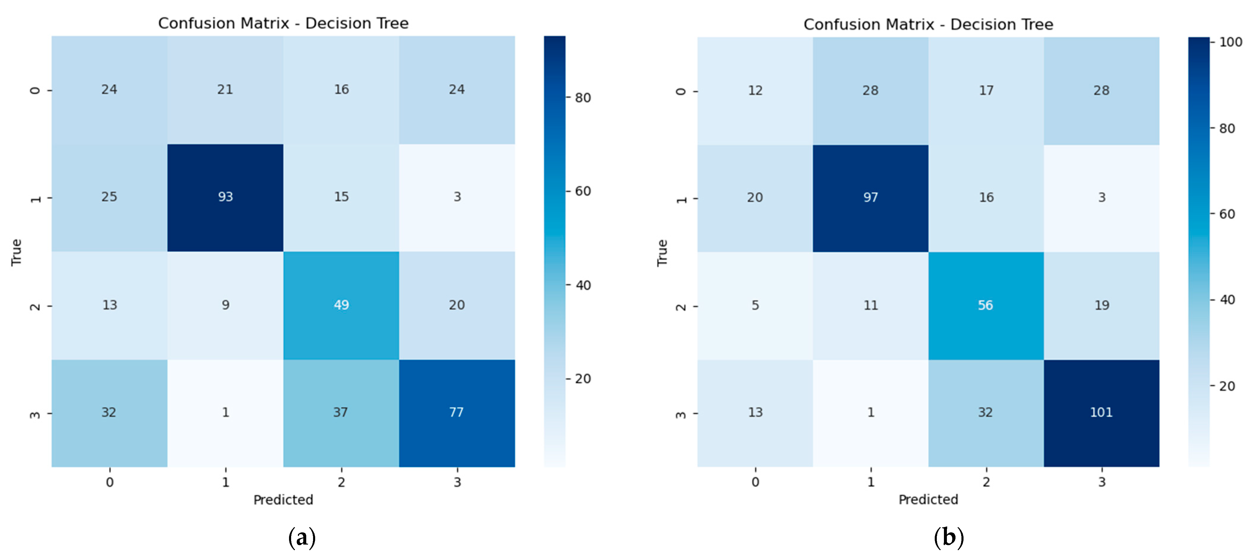
As shown in Figure 9, the confusion matrices illustrate the model’s performance before and after parameter adjustment.

Table 12. Parameters table of the Decision Tree classifier without improved parameters.

Y	Precision	Recall	F1-Score
0	0.26	0.28	0.27
1	0.75	0.68	0.72
2	0.42	0.54	0.47
3	0.62	0.52	0.57

and

Table 13. Parameters table of Decision Tree classifier with improved parameters.

Y	Precision	Recall	F1-Score
0	0.24	0.14	0.18
1	0.71	0.71	0.71
2	0.46	0.53	0.53
3	0.67	0.68	0.68

provide detailed classification results.

The model achieved its strongest outcome when the sensor was placed above the deformed winding (Y1) and reached a precision of 75% in the untuned case and maintained good balance after tuning. Y3 also showed stable performance and confirmed the classifier’s ability to detect deformation when the sensor is near the affected area.

For Y0 and Y2, the precision and F1-scores remained lower, and even after parameter changes, the improvement was minor. This behavior can be explained by the vibration propagation through the winding structure: when the sensor is in Y0 (healthy region), vibration amplitudes remain close to baseline and make discrimination difficult. In Y2 (directly on the defect), local strain distribution becomes highly nonlinear and partly absorbed by contact that produced noisier and less distinctive features. These factors account for the weaker classification performance observed in Y0 and Y2.

The Decision Tree, while easy to interpret, depends heavily on sensor placement. Its results indicate it can be effective in targeted setups where faults are more directly observed.

Overall, the results reveal that sensor position plays a critical role in classification accuracy, regardless of the algorithm used. Across all models, sensor positions Y1 and Y3 consistently yielded higher precision and F1-scores, often exceeding 70%, while Y0 and Y2 resulted in weaker performance. This outcome suggests that detecting vibration patterns above or below the deformed winding provides clearer signals for learning-based classifiers.

Among the models tested, the SVC achieved the highest scores for Y1 and Y3, demonstrating both stability and robustness. Logistic Regression and Decision Tree models also produced reliable outputs, particularly in simpler deformation scenarios, whereas Random Forest and KNN showed greater sensitivity to parameter selection and sensor location.

These findings highlight how critical sensor placement is for achieving reliable transformer monitoring in practical applications. They also suggest that even with modest datasets, machine learning can offer valuable insights when combined with well-designed sensing strategies. The proposed FBG-based sensing offers several advantages such as immunity to electromagnetic interference, suitability for high-voltage environments, compact form factors enabling installation between winding spacers, and stable performance up to 150 °C. These features make optical sensing particularly attractive for online monitoring of transformer windings, where electrical sensors face insulation, noise, and safety limitations. This study focused on frequency-domain features derived from FFT and applied classical supervised learning algorithms (SVM, RF, KNN, etc.) to evaluate feasibility. While this approach is appropriate for early stage validation with limited datasets, we recognize that more advanced methods specifically designed for time-series signals, such as recurrent neural networks, convolutional neural networks, or transformer-based models, may better capture temporal vibration dynamics. Incorporating such models into future work will likely improve classification performance and robustness in real-world transformer monitoring. While this study used a dry-type transformer in a lab environment, future work should examine how these models generalize to oil-filled units or field measurements with environmental noise. Also, expanding the dataset with more deformation types and sensor configurations could further improve model robustness.

5. Conclusions

This experimental study presents a novel approach for the detection and localization of winding deformations in power transformers by integrating optical vibration sensing with machine learning classification. Five supervised learning models were evaluated, with Support Vector Machines demonstrating the most promising performance in identifying specific deformation scenarios (Y1 and Y3) using vibration data. While the achieved classification accuracy of approximately 60% reflects the challenges inherent in early stage modeling, it also establishes a solid foundation for further refinement and development.

A key contribution of this work lies in the use of fiber Bragg grating (FBG) sensors directly mounted on the windings, enabling real-time vibration monitoring without being affected by electromagnetic interference, unlike traditional accelerometers. The strongest vibration signals were observed at the FBG sensors located directly at the deformation site, while sensors positioned above or below the deformation recorded weaker but still elevated signals compared to healthy windings. Furthermore, the farther the FBG is from the deformation, the more damping and phase shift occurs, resulting in progressively weaker signals. These observations confirm the sensor’s sensitivity and its suitability for transformer diagnostics.

Moreover, the custom-designed transformer model enabled controlled simulation of both healthy and deformed winding conditions, providing valuable insights into how mechanical defects influence vibration patterns. This capability to localize relative deformation based on sensor positioning is critical for future fault diagnosis strategies.

Ultimately, this study demonstrates the feasibility of combining optical sensing with machine learning for online transformer health monitoring. With further optimization of the classification models and expanded datasets, this approach holds strong potential for deployment in real-world applications, offering a cost-effective and non-invasive solution for preventing catastrophic transformer failures.