Abstract
An advanced Dyson spectrometer is proposed that redesigns the Dyson prism to make the entire system coaxial and easy to implement for each subassembly, thus greatly enhancing optical design, optical processing, and system alignment. The design concept and fabrication methods, as well as the results of imaging evaluations of the proposed spectrometer, are described in detail. At present, the advanced Dyson spectrometer has been in orbit for more than a year, serving smart agriculture and marine applications. The advanced imaging spectrometer achieves high resolution in both the spectral and spatial directions and low spectral distortion at a high numerical aperture in the working waveband. On the basis of the above research, we have developed three other imaging spectrometers with different performance indicators, including a space-based instrument, an airborne instrument and a ground-based instrument, thus verifying the progress and versatility of advanced Dyson spectrometer technology.
1. Introduction
Imaging spectroscopy in the visible and near-infrared spectral regions is considered an important technique for monitoring and understanding coastal ocean processes such as mapping phytoplankton distributions and seagrass leaf area indices, as well as monitoring algal blooms and coral health [1,2,3,4,5]. Compared with traditional remote sensing imaging technology, hyperspectral imaging technology can obtain high-resolution images while also obtaining narrowband spectral information and can recognize the unique absorption and reflection characteristics caused by the physical properties of target materials through fine spectral segmentation features.
With continuous improvements in aerospace technology, low-cost commercial spectral imaging remote sensing satellites have experienced explosive growth and development. With the introduction of space concepts such as satellite-chain plans, satellite clusters, and constellation networking, more stringent requirements have been initiated for the cost, volume, weight, reliability, and instrument performance of spectral imaging space-based payloads. In addition, to reduce costs further, many commercial satellites have eliminated mechanical vibration, thermal vacuum, thermal equilibrium, and electromagnetic compatibility tests at the component level for spectral imaging instruments through whole-satellite testing verification. Therefore, there is an urgent need to develop a mature, reliable, and advanced spectral imaging system to develop low-cost, high-performance optical space-based payloads that can be easily promoted to the vast commercial satellite market.
At present, mature spectral imaging technology systems provide filter dispersion, interference, curved prism dispersion, and grating dispersion. Filter dispersion spectral imaging technology uses filters for spectral band-selective imaging, which has the drawback of being unable to simultaneously image multiple channels. It is mainly used for multispectral imaging [6]. Interferometric spectral imaging technology uses an interferometer to obtain the interference fringe information of the detection target, which requires spectral restoration to obtain the original spectral data. It has high requirements for the stability and accuracy of the platform and post-image processing [7]. Curved prism dispersion spectral imaging technology uses curved prisms as spectral elements, which are expensive, difficult to process, require high precision, have long processing cycles, and are difficult to assemble and adjust. However, this optical system has high transmittance, so it is mainly used for military reconnaissance applications [8,9]. Grating dispersion spectral imaging technology can use mature commercial grating products as spectral components, making it easy to develop low-cost and short-term hyperspectral imaging instruments. In summary, the prism dispersion has the problems of high optical processing difficulty and high cost. The various types of filter dispersion have the defect of time-division imaging. The Fourier transform-based interferometric imaging technology has the disadvantage of difficult spectral data restoration and high platform stability requirements. The grating dispersion can be utilized in optical system design using commercial grating products, significantly reducing development costs and shortening development cycles. It is the most suitable hyperspectral imaging technology system for commercial satellites [10]. We propose an innovative Dyson hyperspectral imager based on concave grating dispersion [11].
The Dyson spectral imaging system has the advantages of optical path multiplexing, compact structure, and lightweight design. In addition, it also has excellent full-spectrum aberration correction ability, with low distortion and easy implementation of a large relative aperture. In 1959, Dyson first proposed that a simple concentric arrangement of a plano-convex lens and concave mirror would be free of all Seidel aberrations at the design wavelength and center of a field imaged at 1:1 magnification [12]. In the Dyson prototype, the detector image plane and the slit plane are located on the same side of the plano-convex lens, and both coincide. There are two main issues in the prototype of the Dyson structure for engineering implementation. First, the optical window packaging of the detector results in the photosensitive surface of the detector being unable to adhere tightly to the surface of the plano-convex lens. Second, the packaging of the detector structure and circuit board makes the external dimensions of the camera much larger than the size of the detector target surface. However, in the prototype of the Dyson structure, the distance between the target surface and the slit is only a few millimeters, which makes it impossible to achieve spatial arrangements of the camera component, slit component, and front telescope objective component.
To implement the Dyson prototype structure, Pantazis Mouroulis proposed a design approach using glued prisms and fiber optics [13]. This design can alleviate the spatial distribution problem of telescope objective components and detector components, but the spatial allocation of mirrors, fiber optics, and detectors is still insufficient, and the system is complex. David W. Warren proposed the introduction of a meniscus lens, which allows the surfaces of objects and images to be appropriately pulled out of the surface of the plano-convex lens and adds a small reflector behind the slit surface [14]. This solution significantly improves the spatial layout of the Dyson prototype structure, but because the object surface and image surface are still on the same side of the plano-convex lens, the installation and adjustment of the optomechanical structure are difficult in a tight engineering layout. Pantazis Mouroulis also proposed a similar design form, which uses mirrors to bend the slit and telescope objective light path at an angle to adjust the spatial position distribution of the detector and telescope objective [15]. However, there is still the problem of an insufficient spatial layout of the mirrors and detectors. Pantazis Mouroulis [16] and William R. Johnson [17] subsequently proposed another design form, which involved designing Dyson prisms as irregular parts and processing reflective surfaces to bend the optical path, thereby separating the image plane from the object plane. However, the above two design forms introduce the problem of irregular prism processing. The proposed Dyson prism has an irregular convex surface at the incident end of the object surface. The internal reflection surface of the Dyson prism and the edge of the light exit surface in front of the image face both have corners, which cannot be machined and polished. Moreover, ensuring the flatness and smoothness of the surface near the corner is difficult, resulting in high processing costs and a low yield of Dyson prisms. In addition, the correction mirror group and concave grating behind the Dyson prism are not coaxial optical systems, making instrument installation and adjustment difficult.
On the basis of the above shortcomings and deficiencies, an advanced Dyson hyperspectral imaging technique is proposed, in which all surfaces of the Dyson prism are convex flat surfaces without small convex platforms, eliminating all edge corners of the transmission and reflection surfaces. The incident surface and exit surface of the prism are perpendicular, and the reflective surface maintains a standard angle of 45° with the incident and exit surfaces. It is easy to process and has a simple coating process. The system is a coaxial optical system that is easy to fabricate and test and can be mass-produced at a low cost. On the basis of the above technology, we completed the development of a series of products in Section 5, which we applied to aerospace, aviation, and ground use.
The organization of the paper is as follows: Section 2 describes the optical design and analysis of the advanced Dyson spectrometer. The fabrication and alignment of the instrument are introduced in Section 3. In Section 4, the performance assessment of the imaging spectrometer is described in detail. Section 5 provides the promotion and application of serialized products via this technique. Finally, the discussion and conclusions of the study are presented in Section 6 and Section 7, respectively.
2. Optical Design and Analysis of the Spectrometer
2.1. Imaging Characteristics Analysis of the Dyson Imaging Structure (DIS)
The DIS consists of a plano-convex thick lens and a concave mirror. The radii of the convex surface of the plano-convex lens and the concave surface of the concave mirror are r and R, respectively. These two surfaces share a common center C, as shown in Figure 1a. The concave reflector serves as the system aperture and is located on the focal plane of the plano-convex thick lens.
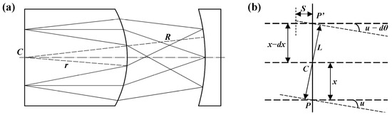
Figure 1.
Imaging characteristics of the DIS: (a) schematic diagram of the DIS, where n is the plano-convex thick lens; (b) object image relationship of the DIS in the nonparaxial optical path.
The radius of a concave mirror, R, can be calculated as
If the object point is located at the common center of the DIS, the light will pass through the center of the sphere without deviation, and the system’s spherical aberration will be zero. If the object point is not located at the center of the sphere, but the system satisfies the sine condition, the coma is zero. Compared with the aperture (i.e., concave mirror), the distortion of the DIS is zero because of the rotational symmetry of the front and rear optical paths. Under the near-axial condition of the DIS, the Petzval sum can be expressed as
By substituting Equation (1) into Equation (2), the Petzval sum of the DIS can be obtained:
The field curvature of the DIS under near-axial conditions is zero. Since any object point in the DIS is imaged on a straight line passing through the object point and point C, the sagittal field curvature on the image plane is zero. Moreover, the Petzval curvature of the DIS is also zero, which implies that the meridian field curvature is also zero. Therefore, the DIS does not exhibit astigmatism.
However, there are high-order aberrations in the nonparaxial optical path of the DIS. The Petzval curvature of the DIS is not zero, and the sagittal field curvature on the image plane is zero. Therefore, the main aberration of the DIS is the meridian field curve. The DIS does not produce an axial aberration, coma or sagittal field curve, and the distortion is related only to the absorption of different light waves by the medium in the object space and image space. However, the DIS has a meridian field curve, and the meridian field curve can be corrected via optimization [18].
There is a deviation angle between the incident light and the outgoing light in the nonparaxial optical path of the DIS, as shown in Figure 1b. The deviation distance between the actual position of the light emitted from the rear surface of the thick lens and the ideal position, dx, can be expressed as
where P is the object point, P′ is the image point, L is the distance from the common spherical center C to the incident light and the outgoing light, and n is the refractive index of the lens.
The distance between the ideal image plane and the real image plane, s, can be expressed as
The above formula shows that the influence of the field of view on the image plane offset is much greater than that of the aperture angle. Therefore, the DIS can achieve high-quality imaging under a large aperture angle.
2.2. Aberration Characteristic Analysis of the Dyson Spectrometer
The Dyson spectrometer is a concentric optical structure, with the grating surface serving as the system aperture. The analysis of its aberration characteristics is based on the wavefront aberration model of the concentric optical system and introduces the influence of dispersion gratings, as shown in Figure 2. The coordinate system is established in the Dyson spectrometer with the common center C of the surface as the coordinate origin. XCY is the object plane and the image plane, with the z-axis perpendicular to the XCY plane and along the optical axis direction. O (x1, y1) is the object point, and I (x2, y2) is the image point of O. R is the curvature radius of the grating. Pg is the center of the grating and is located on the z-axis. The direction of the grating lines is parallel to the x-axis. Qg (X, Y) is any point on the surface of the grating. Ig is the vertical distance from Qg to the optical axis.
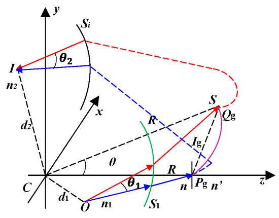
Figure 2.
Influence of gratings on concentric optical structures.
According to Hamilton’s wavefront aberration theory, the sum of the optical path difference (OPD) in concentric optical systems can be expressed by the following formula:
The OPD introduced by concave grating can be expressed as [18]
where N (X, Y) represents the difference in the number of grating lines at points Pg and Qg. M is the diffraction order, and λ is the selected wavelength.
Therefore, the wavefront aberration at image point I of the Dyson spectrometer is the sum of the OPD of the concentric optical system and the OPD introduced by the grating:
The above equation reflects the difference between the actual wavefront and the ideal wavefront of light with a wavelength of λ emitted from point O, passing through a point Qg on the grating, and reaching the image plane. Because the concentric spectral imaging system is a dual telecentric system, both the object space and the image space are plane waves. The pupil wavefront aberration generated by the light passing from the object space to the grating is represented as , and the pupil wavefront aberration generated by the light passing through the grating to the image space is represented as .
Assuming that the light emitted from the center Pg of the grating toward point O passes through a series of concentric spheres and media as a plane wave perpendicular to the optical axis to reach point O, according to the Hamilton function and the axial symmetry of the concentric system, the wavefront aberration generated by the light reaching point O is a function of the distance between point O and center C:
Assuming that the light emitted from the off-axis point Qg on the grating to point O passes through a series of concentric spheres and media as a nearly plane wave to reach point O, and that the angle between the reference wave of the object plane and the object space is θ, then
The numerical aperture of the system in the object space is . Moreover, the angle between the reference wave in the object space and CO is assumed to be θ1. The distance between the reference wave from point Qg to point O and center point C of the system when it intersects is d1sinθ. According to the characteristics of concentric optical systems, the wavefront aberration at point O becomes .
The following relationships exist in concentric optical systems:
Rewriting Equations (13) and (14) yields
By the same principle, the wavefront aberration generated from point Qg and point Pg to point I can be calculated as follows:
where θ2 is the angle between the wave emitted from point Qg and the CI when it passes through a series of optical surfaces and media between Qg and I and reaches the image space.
In summary, in the Dyson spectrometer, the wavefront aberration generated by the light wave emitted from point O to its corresponding image point I is as follows:
where W0 is the inherent wave aberration of a concentric optical system, which contains only aberration terms above the second power and can be ignored.
From the triangle relationship and the grating equation, the following conclusions can be drawn:
By substituting Equation (16) into Equation (15), we can obtain
The relationship is the wave aberration result of the Dyson spectrometer. As seen from the above equation, the variation in the wavefront aberration in the Dyson spectrometer is related to the line density of the spherical grating, diffraction order, and diffraction wavelength. When the grating has equidistant parallel grooves, no additional wavefront aberration is introduced. The addition of a Rowland grating to the Dyson spectrometer still results in concentricity, giving it a significant advantage in terms of aberration control. However, because the diffraction grating diffracts light of different wavelengths at different positions, the system loses the symmetry of the diffraction direction, which will cause certain astigmatisms at different wavelength positions. This astigmatism can be optimized by changing the radius of the convex surface of the flat convex thick lens and adjusting the distance between the thick lens and the grating appropriately. Owing to the presence of the refracted lens, the system produces color differences. Two materials can be glued together, or a crescent lens can be added to correct the color difference.
2.3. Initial Parameter Calculation of the Dyson Spectrometer
To effectively control the astigmatism of the Dyson spectrometer, a design method for dual-wavelength astigmatic imaging at the longest and shortest wavelengths in the working wavelength range was proposed [19].
An imaging schematic diagram of the principal ray diffraction path at any wavelength in the sagittal and meridional planes is shown in Figure 3. If the system can achieve ideal imaging, the sagittal image point should coincide with the meridional image point, and the astigmatism should be zero, that is, δ = 0.
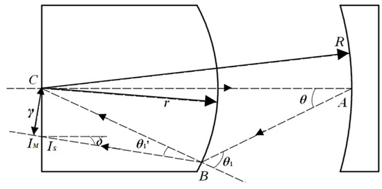
Figure 3.
Diffraction path of any wavelength principal ray in the sagittal and meridional planes. R and r are the radius of the concave reflection grating and the convex radius of the flat convex thick lens, respectively. C is the common center of the concentric system. θ is the diffraction angle at any wavelength. θ1 is the incident angle of diffracted light on the convex surface of a plano-convex lens. θ1’ is the exit angle of diffracted light on the convex surface of a plano-convex lens. IM and IS represent the image points of diffracted light on the meridional and sagittal planes, respectively. δ represents the angle between the ray at the meridian image point and the normal of the back surface of the plano-convex thick lens. A is the intersection point between the incident light and the grating surface, and B is the intersection point between the diffracted light and the convex surface of the lens. n is the refractive index of a plano-convex lens.
From the direct relationship between the angles in the figure, the following can be seen:
According to the triangular sine theorem and Snell’s law,
By substituting Equation (19) into the grating equation, we can obtain
When the stigmatic condition δ = 0 is satisfied, :
By inverting and squaring the numerator and denominator of the above formula, it can be rewritten as
According to the Taylor expansion of the grating equation, we can obtain
By substituting Equation (23) into Equation (22), we can obtain
Take two wavelengths λa and λb as the stigmatic wavelengths, input them into the above equation and subtract them to obtain the stigmatic parameters at the two wavelengths. When the diffraction order m = 1, the dual-wavelength stigmatic equation can be formulated as
where na and nb are the refractive indices of wavelengths λa and λb, respectively. The above formula can be used to calculate the grating constant when two wavelengths are stigmatic. Furthermore, the grating constant can be calculated on the basis of the spectral broadening at the image plane via Equation (26).
Through the above derivation, the optical imaging characteristics of the Dyson structure and the aberration characteristics of the Dyson spectrometer were systematically analyzed, and it was found that the Seidel aberration of the Dyson structure was zero and that the grating with equal density did not introduce additional aberrations. Furthermore, the formula derivation of the initial structural parameters of the Dyson spectrometer was completed. Under the condition of considering astigmatism, we then utilized ZEMAX 2019 to determine the distribution of the power to suppress spherical aberrations and chromatic aberrations to further optimize the Dyson spectrometer on the basis of the above analysis.
2.4. Optical Design Results of the Advanced Dyson Spectrometer (ADS)
The optical design was analyzed to confirm its imaging performance and is presented in Figure 4. The ADS can be divided into a telescope subassembly and spectral subassembly. The telescope subassembly is a transmissive coaxial lens that uses three materials: CAF2, H-LAK2A, and TF3. The slit uses optical etching and chrome plating technology. An optical filter is designed in front of the slit to prevent excess objects from falling on the slit and to cut off the spectral range in the serialized products (in Section 5).
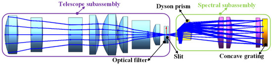
Figure 4.
Optical layout of the ADS.
The spectral subassembly consists of 5 optical elements, including a modified Dyson prism, three correction lenses and a concave grating. The modified Dyson prism differs from all Dyson prisms proposed in previous studies. The incident surface and exit surface of the modified Dyson prism are perpendicular, whereas the reflective surface maintains a standard angle of 45° with both the incident and exit surfaces, greatly reducing the difficulty of fabrication and alignment. The material of the modified Dyson prism is silica, and the refractive index n is 1.456. The optimized parameters of the ADS are shown in Table 1.

Table 1.
The optimized parameters of the ADS.
Figure 5 shows the simulation and analysis of the full-field MTF of an ADS with different wavelengths. The simulations revealed that the minimum MTF of the ADS was 0.82 at 36.5 lp/mm. The spot diagram in Figure 6 shows the spatial resolution of the imaging system, with significant differences found for different FOVs of the ADS under different wavelengths. The average root-mean-square (RMS) diameter was ~8.5 μm, which was much smaller than the pixel size. To ensure that the optical imaging system has good imaging quality, the spectral distortion of the ADS is analyzed, and the results are shown in Figure 7. The maximum spectral smile distortion and keystone distortion were less than 0.20 pixels in the effective FOV. These results demonstrate that the proposed ADS would exhibit excellent imaging performance.
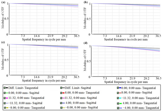
Figure 5.
MTF of ADS at different wavelengths. MTF of full field of view at (a) 0.4 μm, (b) 0.6 μm, (c) 0.75 μm, and (d) 0.9 μm.
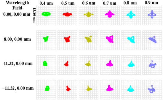
Figure 6.
Spot diagram of the ADS.
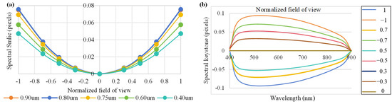
Figure 7.
Spectral (a) smile distortion and (b) keystone distortion of the ADS at full FOV.
3. Fabrication and Alignment
3.1. Engineering Design of Optomechanical Structure
By adopting a modular design approach, the ADS can be divided into a telescope subassembly, Dyson prism subassembly, rear-lens subassembly, grating subassembly, detector subassembly, and integrated box subassembly. Each subassembly was integrated and installed on the integrated box via an adjustment pad, which was used to adjust the spatial position and posture of each subassembly. The optomechanical layout of the ADS is shown in Figure 8. The entire frame was made of type 2A12T4 aluminum, except for the adhesive seat of the Dyson prism, which was made of titanium alloy. The overall size of the ADS was 530 × 211 × 159 mm, and the weight of the ADS was 10.2 kg. The ADS has 6-way thermal controls that can maintain the working temperature at 20 ± 2 °C to achieve good imaging quality. The ADS was installed as a standalone device on the satellite platform, with its flight direction perpendicular to the slit direction.
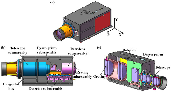
Figure 8.
Optomechanical layout of the ADS: (a) structure of the entire ADS; (b) installation diagram inside the box; (c) profile of the ADS. The Z direction was the direction of the Earth observation, which was parallel to the optical axis. The Y direction was determined by the direction of the slit, and the X direction was taken as the flight direction.
The Dyson prism was the core component of the ADS, which was fixed by bonding the bottom surface with epoxy adhesive. During the bonding process, the two mutually perpendicular planes of the Dyson prism were initially positioned through the bonding fixture to ensure positional accuracy in system alignment. The detector subassembly consists of two printed circuit boards with a spacing of 25 mm. The concave grating was connected to the box as a separate subassembly for easier multiple degrees of freedom adjustment. The integrated box was iteratively optimized to combine structural strength and lightweight advantages. Its upper and side cover plates could be disassembled for easy installation of various subassemblies inside the box.
3.2. Alignment and Assembly
The ADS is a coaxial spectral imaging system, with the telescope subassembly and spectral subassembly having parallel optical axes and a horizontal distance of 1 mm between the two optical axes. Owing to the improved design of the Dyson prism, the alignment difficulty of the entire system has been significantly reduced. The system integration process mainly includes the following three steps: telescope subassembly integration, spectral subassembly integration, and system fine-tuning. Thus, aligning the ADS is performed via the following steps:
- (1)
- Integration of the telescope subassembly
- (a)
- Installing each lens into the frame, applying glue, and curing.
- (b)
- Centering the processing technology to ensure the coaxiality of each lens.
- (c)
- Using a Zogy interferometer to measure the surface shape errors of each lens, ensuring that the surface shape errors (RMSs) are less than (1/40) λ.
- (d)
- Adjusting the spacer thickness to ensure the air distance between each lens.
- (2)
- Integration of the spectral subassembly
- (a)
- Installing the Dyson prism subassembly, rear-lens subassembly, and grating subassembly at theoretical intervals.
- (b)
- Installing the detector subassembly and fine-tuning the position of the image plane to maintain clear imaging.
- (c)
- Rotating the grating and fine-tuning the phase of the grating.
- (3)
- System fine-tuning
- (a)
- Installing the telescope subassembly on the box and finely adjusting the image plane on the slit surface of the spectral subassembly.
- (b)
- Fine-tuning the direction of the slit to ensure it is perpendicular to the installation surface of the box.
- (c)
- Testing the ADS and ensuring that the indicators meet the requirements via precise adjustment of the slit, detector and grating.
- (d)
- Presetting the position of the vacuum image plane and replacing and adjusting the thickness of the pad to achieve clear imaging in a vacuum environment.
- (e)
- Cleaning up excess materials, implementing thermal controls, and performing adhesive curing (as shown in Figure 9).
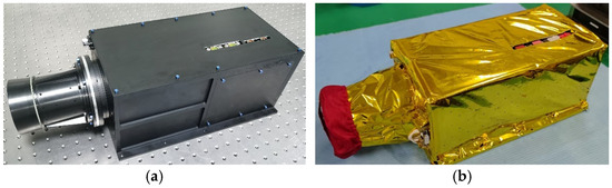 Figure 9. Assembly of the ADS: (a) integration is complete; (b) implementation of thermal control.
3.3. Vibration Test
During the launch process, the space-based ADS was subjected to complex mechanical vibrations. According to the simulation analysis of the sinusoidal vibration test, the first natural frequency of the ADS was much higher than 100 Hz. According to the simulation analysis of sinusoidal vibration test, the first natural frequency of ADS was much higher than 100 Hz and would not resonate with the satellite platform during launch. Hence, there was no need to perform a sinusoidal vibration test, and only a random mechanical test was performed on the ADS to ensure the stability of the ADS imaging performance. The random vibration mechanics conditions of the ADS are shown in Table 2.
Table 2.
Random vibration test conditions of the ADS.
Figure 10 shows the random vibration process of the ADS. The random mechanical test results revealed that the natural frequency of the ADS was 552.7 Hz, and the maximum amplification of the total acceleration in the three directions was 4.43. The modulation transfer function (MTF) was retested before and after the vibration test, and there was no change, indicating that the ADS had excellent mechanical stability.
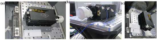
Figure 10.
Random mechanical test of the ADS. (a) Random mechanical test of the ADS in the X direction. (b) Random mechanical test of the ADS in the Y direction. (c) Random mechanical test of the ADS in the Z direction.
4. Performance Assessment
4.1. Spectral Performance Test
After the integration and alignment of the ADS was completed, its spectral performance was tested, mainly including its spectral resolution, center wavelength and spectral smile. These indicators are important spectral performance parameters of imaging spectrometers and directly affect the spectral accuracy of the spectrometer.
We used the Model 207 monochromator from McPherson Corporation in the Boston, MA, USA to output a fixed-wavelength monochromatic laser for measuring the spectral resolution of the ADS. Its own spectral resolution is 0.08 nm, and the spectral range is 185–2600 nm, which can cover the measurement range of the ADS. For this test, four specific wavelengths, 500 nm, 600 nm, 700 nm, and 800 nm, were selected for spectral resolution testing. The image acquisition results are shown in Figure 11.

Figure 11.
Spectral resolution image acquisition overlay results and images of monochromatic lasers at 500 nm, 600 nm, 700 nm, and 800 nm from top to bottom.
For each specific wavelength mentioned above, spectral responses within the range of ± 4 nm at continuous intervals of 0.5 nm were collected to fit the spectral response curve. The spectral resolution at that wavelength can be obtained by calculating the full width at half maximum of the Gaussian function fitted by the spectral response curve. The spectral resolution calculation results are shown in Figure 12. The average spectral resolution of the ADS was 3.18 nm, which meets the requirement of a spectral resolution of less than 3.5 nm.
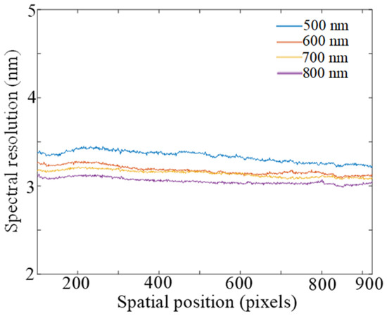
Figure 12.
Spectral resolution fitting results for 4 specific wavelengths.
On the basis of the above results, the center of symmetry of the Gaussian function can be calculated to determine the center wavelength corresponding to the current spectral channel. The center wavelength of each channel can be obtained by linearly fitting the center wavelength with the corresponding detector pixel position, as shown in Figure 13. Through analysis, it is shown that there is a linear correspondence between the center wavelength of the ADS and the position of the detector pixels, with a total of 157 bands distributed at equal intervals in the ADS.
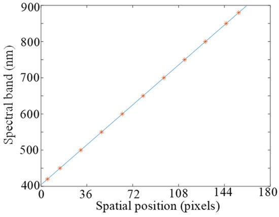
Figure 13.
Relationship of the ADS between the center wavelength and the pixel position.
The spectral smiles in the four bands mentioned above were tested, and the results are shown in Figure 14. The maximum difference in the spectral smiles of the test bands should not exceed 0.2 pixels. The analysis results show that the ADS has excellent spectral performance.
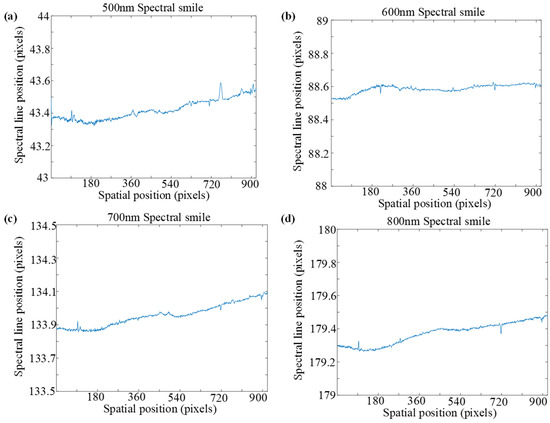
Figure 14.
The spectral smiles of the ADS at different wavelengths. (a) 500 nm. (b) 600 nm. (c) 700 nm. (d) 800 nm.
4.2. Imaging Performance
The imaging performance of the ADS was verified through external field push–scan experiments. The ADS was installed on a two-dimensional high-precision turntable and rotated at a constant speed to drive the ADS to finish the push–scan imaging. The hyperspectral data obtained are shown in Figure 15.
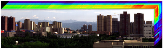
Figure 15.
Data cube obtained from push–scan tests of the ADS.
The push–scan image was clear, and the image feature edges were neat. The proportion of ground objects in the hyperspectral data was moderate without deformation. To verify the spectral accuracy of the ADS, an external spectral curve accuracy test was conducted. When conducting external field imaging experiments, a white board with 99% reflectivity and a gray board with 50% reflectivity were placed in the imaging field of the ADS to obtain hyperspectral data containing both (as shown in Figure 16). The true spectral curves of the two diffuse reflection plates were measured by a qualified ASD portable ground spectrometer. The spectral accuracy of the ADS is characterized by the deviation between the ADS-reconstructed spectral curve and the true spectral curves obtained by the ASD portable ground spectrometer.

Figure 16.
Spectral accuracy testing of the ADS: calculating the absolute calibration coefficient using a white board with 99% reflectance and a gray board with 50% reflectance as the target for spectral accuracy testing.
For practical calculations, the first step involved obtaining two sets of spectral curves of the 99% reflectance white board via the ADS and ASD portable ground spectrometer. The absolute calibration coefficient of the ADS was subsequently calculated from both datasets. The spectral curve of the 50% reflectance gray board measured by ADS was corrected via the above absolute calibration coefficient to obtain its reconstructed spectral curve. Finally, by comparing the reconstructed spectral curve of the 50% reflectance gray board with the spectral curve measured by the ASD portable ground spectrometer, the relative deviation between the two was obtained, which could be defined as the spectral accuracy of the ADS. The test results are shown in Figure 17, which indicates that the relative deviation of the spectral curve accuracy of the gray board with 50% reflectance in the full spectral range of the ADS was 2.04%. Imaging performance tests indicated that the ADS had excellent hyperspectral imaging performance, which also confirmed the feasibility of the design method proposed in this study.
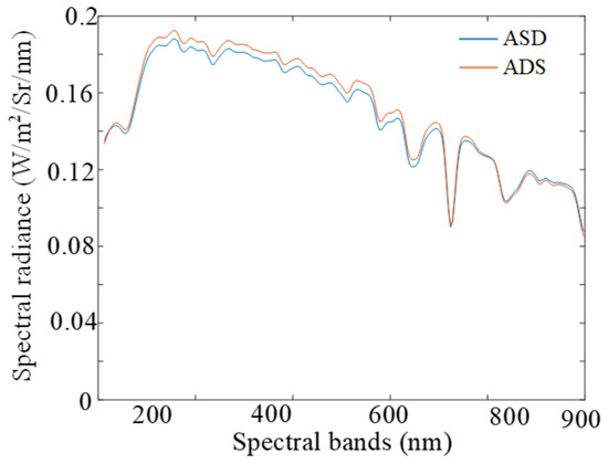
Figure 17.
Test accuracy of the spectral curve of the 50% reflectance gray board by the ADS.
The ADS we designed was successfully launched and entered its designated orbit on 9 January 2023. It has been in orbit for more than a year and has successfully transmitted hyperspectral data. Some of the publicly available data are shown in Figure 18. The imaging quality of the ADS in orbit is stable and clear, and it has been applied in many traditional and emerging industries, such as ocean imaging and smart agriculture.
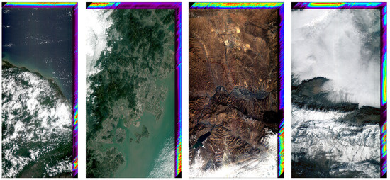
Figure 18.
Partial in-orbit hyperspectral data of the ADS.
5. Promotion and Application of Serialized Products
Based on the ADS proposed in this article, different spatial resolutions can be achieved by changing the design of a telescope subassembly, and the transmission bandwidth of the filter in front of the slit can be changed to achieve spectral band selection in the range of 400–1000 nm. The spectral resolution of the instrument can be changed by changing the number of merged pixels in the spectral dimension of the detector. By implementing the above adjustments, it is easy to achieve customized designs of spectral imaging instruments to meet the needs of different application scenarios.
To further validate the ADS technology, we developed a space-based imaging spectrometer, a ground-based imaging spectrometer, and an airborne imaging spectrometer (Figure 19). All three imaging spectrometers have completed alignment, performance testing, and data application, achieving excellent imaging performance. The detailed design of these three instruments will be described in subsequent articles. A detailed comparison of the technical specifications of the four spectral instruments proposed in this article is shown in Table 3.
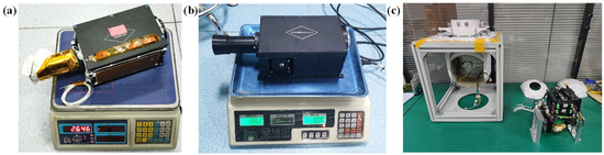
Figure 19.
Three additional spectral imaging devices based on ADS technology: (a) space-based imaging spectrometer; (b) ground-based imaging spectrometer; (c) airborne imaging spectrometer.
Table 3.
Comparison of the characteristic specifications of the four spectral instruments.
Through the development of the abovementioned instruments, it has been verified that ADS technology can achieve excellent spectral imaging performance, can offer lightweight and compact designs, and is easy to mount on various aviation and aerospace platforms. In addition, the core dispersion element of the system uses commercial grating products from Jobin Yvon, which have the advantages of low cost and are easy to mass-produce.
6. Discussion
The ADS utilized the Dyson spectrometer with optical path multiplexing based on concave grating dispersion elements. We provided a detailed discussion on the proposed ADS from several aspects, including optical principles, optical design, structural design, adaptability analysis of on-board environment, integration and alignment, and performance testing. The ADS achieved spectral detection with a maximum width of 400–1000 nm, a minimum spectral resolution of 2.86 nm and a F-number of 2.2. The minimum spectral distortion could reach 0.1 pixels, with excellent spectral performance and an accuracy of 2.04% compared to standard radiometer measurements. Our core innovation lies in improving the design configuration of the Dyson prism, which significantly enhances system performance and reduces development difficulty. The ADS we designed completed on-board application and verification, and had good imaging quality.
The well-known and typical spectral imaging instruments mainly included the Portable Hyper-spectral Image for Low-Light Spectroscopy (PHILLS) [20], Portable Remote Imaging Spectrometer (PRISM) [15] and Advanced airborne hyperspectral imaging system (AAHIS) [21]. A comparison between the published works and our ADS has been presented in Table 4. The core advantage of the ADS lies in its high spectral resolution while maintaining consistent performance indicators. It was developed using commercial gratings and had low development costs.
Table 4.
Comparison of the comparison of primary specifications.
7. Conclusions
To summarize, we propose an advanced Dyson spectrometer technology and provide a detailed and engineering explanation of its characteristics. The core innovation of the system lies in the design of the advanced Dyson prism, which makes the entire system coaxial and easy to implement for each subassembly, greatly enhancing optical design, optical processing, and system alignment. On the basis of the above technical research, four imaging spectrometers with different technical indicators have been developed, including two spaceborne spectrometers, one unmanned airborne spectrometer and one ground spectrometer. All four instruments have achieved lightweight, low-cost designs and excellent spectral imaging performance, thus verifying the progress and versatility of the advanced Dyson spectral technology proposed in this paper. The proposed design concepts, alignment process, and verification methods contribute to research on the hyperspectral remote sensing of oceans and coasts. Further research on imaging spectrometers will focus on the following steps: (1) expanding the imaging spectrum to the ultraviolet band; (2) reducing optical components and introducing high-diffraction-efficiency gratings to improve the instrument signal-to-noise ratio and facilitate weak signal detection in the ocean; and (3) expanding the application scenarios of advanced Dyson imaging spectrometers.
8. Patents
Chinese patent: A Small and Lightweight Dyson Hyperspectral Imaging System for Spaceborne Applications (CN113155285A).
Author Contributions
Conceptualization, X.J. (Xinyin Jia) and S.L.; Data curation, Z.Z.; Formal analysis, J.L.; Funding acquisition, X.J. (Xinyin Jia); Investigation, J.L.; Methodology, X.J. (Xinyin Jia) and X.H.; Project administration, X.J. (Xinyin Jia); Resources, S.L. and X.J. (Xin Jiang); Software, Z.Z. and P.H.; Supervision, Z.Z.; Visualization, X.H.; Writing—original draft, X.J. (Xinyin Jia) and X.J. (Xin Jiang); Writing—review & editing, X.J. (Xinyin Jia). All authors have read and agreed to the published version of the manuscript.
Funding
This research was funded by National Natural Science Foundation of China under Grant 42306202 and China Postdoctoral Science Foundation under Grant 2024M763919.
Institutional Review Board Statement
Not applicable for studies not involving humans or animals.
Data Availability Statement
The original contributions presented in this study are included in the article. Further inquiries can be directed to the corresponding authors.
Conflicts of Interest
The authors declare that they have no known competing financial interests or personal relationships that could have appeared to influence the work reported in this paper.
Abbreviations
The following abbreviations are used in this manuscript:
| ADS | Advanced Dyson spectrometer |
| DIS | Dyson imaging structure |
References
- Yu, L. Upgrade of a UV-VIS-NIR imaging spectrometer for the coastal ocean observation: Concept, design, fabrication, and test of prototype. Opt. Express 2017, 25, 15526–15538. [Google Scholar] [CrossRef] [PubMed]
- Jia, X.; Li, S.; Ke, S.; Hu, B. Overview of spaceborne hyperspectral imagers and the research progress in bathymetric maps. In Second Target Recognition and Artificial Intelligence Summit Forum; SPIE: Bellingham, WA, USA, 2020; Volume 11427, pp. 118–124. [Google Scholar]
- Davis, C.; Carder, K.; Gao, B.-C.; Lee, Z.-P.; Bissett, W. The development of imaging spectrometry of the coastal ocean. In Proceedings of the 2006 IEEE International Symposium on Geoscience and Remote Sensing, Denver, CO, USA, 31 July–4 August 2006; IEEE: New York, NY, USA, 2006; pp. 1982–1985. [Google Scholar]
- Harringmeyer, J.P.; Ghosh, N.; Weiser, M.W.; Thompson, D.R.; Simard, M.; Lohrenz, S.E.; Fichot, C.G. A hyperspectral view of the nearshore Mississippi River Delta: Characterizing suspended particles in coastal wetlands using imaging spectroscopy. Remote Sens. Environ. 2024, 301, 113943. [Google Scholar] [CrossRef]
- Dierssen, H.M.; Zimmerman, R.C.; Leathers, R.A.; Downes, T.V.; Davis, C.O. Ocean color remote sensing of seagrass and bathymetry in the Bahamas Banks by high-resolution airborne imagery. Limnol. Oceanogr. 2003, 48, 444–455. [Google Scholar] [CrossRef]
- Garini, Y.; Young, I.T.; McNamara, G. Spectral imaging: Principles and applications. Cytom. Part A J. Int. Soc. Anal. Cytol. 2006, 69, 735–747. [Google Scholar] [CrossRef] [PubMed]
- Vakhtin, A.B.; Peterson, K.A.; Wood, W.R.; Kane, D.J. Differential spectral interferometry: An imaging technique for biomedical applications. Opt. Lett. 2003, 28, 1332–1334. [Google Scholar] [CrossRef] [PubMed]
- Wen, M.; Wang, Y.; Yao, Y.; Yuan, L.; Zhou, S.; Wang, J. Design and performance of curved prism-based mid-wave infrared hyperspectral imager. Infrared Phys. Technol. 2018, 95, 5–11. [Google Scholar] [CrossRef]
- Jia, X.Y.; Li, X.J.; Hu, B.L.; Li, L.B.; Wang, F.C.; Zhang, Z.H.; Yang, Y.; Ke, S.L.; Zou, C.B.; Liu, J.; et al. Comprehensive design analysis and verification of space-based short-wave infrared coded spectrometer via curved prism dispersion. Appl. Opt. 2022, 61, 2125–2139. [Google Scholar] [CrossRef] [PubMed]
- Xue, Q.; Gao, X.; Lu, F.; Ma, J.; Song, J.; Xu, J. Development and Application of Unmanned Aerial High-Resolution Convex Grating Dispersion Hyperspectral Imager. Sensors 2024, 24, 5812. [Google Scholar] [CrossRef] [PubMed]
- Jia, X.Y.; Zou, C.B.; Yang, F.C.; Yan, P.; Li, S.Y.; Hu, B.L. A small and lightweight on-board Dyson hyperspectral imaging system. China Patent CN113155285A, 23 July 2021. [Google Scholar]
- Dyson, J. Unit magnification optical system without Seidel aberrations. J. Opt. Soc. Am. 1959, 49, 713–716. [Google Scholar] [CrossRef]
- Mouroulis, P.Z.; Green, R.O. Optical design for imaging spectroscopy. In Current Developments in Lens Design and Optical Engineering IV; SPIE: Bellingham, WA, USA, 2003; Volume 5173, pp. 18–25. [Google Scholar]
- Warren, D.W.; Gutierrez, D.J.; Keim, E.R. Dyson spectrometers for high-performance infrared applications. Opt. Eng. 2008, 47, 103601. [Google Scholar] [CrossRef]
- Mouroulis, P.; Van Gorp, B.E.; Green, R.O.; Eastwood, M.; Wilson, D.W.; Richardson, B.; Dierssen, H. The portable remote imaging spectrometer (PRISM) coastal ocean sensor. In Optical Remote Sensing of the Environment; Optica Publishing Group: Washington, DC, USA, 2012. [Google Scholar]
- Mouroulis, P.; Green, R.O.; Wilson, D.W. Optical design of a coastal ocean imaging spectrometer. Opt. Express 2008, 16, 9087–9096. [Google Scholar] [CrossRef] [PubMed]
- Johnson, W.R.; Hook, S.J.; Shoen, S.M. Microbolometer imaging spectrometer. Opt. Lett. 2012, 37, 803–805. [Google Scholar] [CrossRef] [PubMed]
- Wynne, C.G. Monocentric telescopes for microlithography. Opt. Eng. 1987, 26, 300–303. [Google Scholar] [CrossRef]
- Montero-Orille, C.; Prieto-Blanco, X.; González-Núñez, H.; de La Fuente, R. Design of Dyson imaging spectrometers based on the Rowland circle concept. Appl. Opt. 2011, 50, 6487–6494. [Google Scholar] [CrossRef] [PubMed]
- Davis, C.O.; Bowles, J.; Leathers, R.A.; Korwan, D.; Downes, T.V.; Snyder, W.A.; Reisse, R.A. Ocean PHILLS hyperspectral imager: Design, characterization, and calibration. Opt. Express 2002, 10, 210–221. [Google Scholar] [CrossRef] [PubMed]
- Topping, M.Q.; Pfeiffer, J.E.; Sparks, A.W.; Jim, K.T.; Yoon, D. Advanced airborne hyperspectral imaging system (AAHIS). In Imaging Spectrometry VIII; SPIE: Bellingham, WA, USA, 2002; Volume 4816, pp. 1–11. [Google Scholar]
Disclaimer/Publisher’s Note: The statements, opinions and data contained in all publications are solely those of the individual author(s) and contributor(s) and not of MDPI and/or the editor(s). MDPI and/or the editor(s) disclaim responsibility for any injury to people or property resulting from any ideas, methods, instructions or products referred to in the content. |
© 2025 by the authors. Licensee MDPI, Basel, Switzerland. This article is an open access article distributed under the terms and conditions of the Creative Commons Attribution (CC BY) license (https://creativecommons.org/licenses/by/4.0/).