1. Introduction
Numerous studies have demonstrated that metabolic abnormalities may be a key pathogenic factor in cancer [
1]. For instance, impaired macrophage phagocytosis contributes to tumor susceptibility induced by psychological stress [
2]. Hormonal dysregulation caused by anxiety and depression increases the incidence of breast cancer [
3]. Moreover, even in the extremely early stages of breast tumor development before morphological formation, rapid cell division leads to localized metabolic abnormalities, including hyperperfusion, hypoxemia, and angiogenesis [
4]. Currently, multiple clinical modalities are available for blood flow detection, each with inherent limitations. For instance, ultrasound Doppler is restricted to large-vessel hemodynamic assessment [
5]; laser Doppler flowmetry (LDF) and laser speckle contrast imaging (LSCI) are limited to superficial tissue monitoring [
6]; perfusion magnetic resonance imaging (pMRI) faces challenges due to high operational costs and lack of intraoperative compatibility [
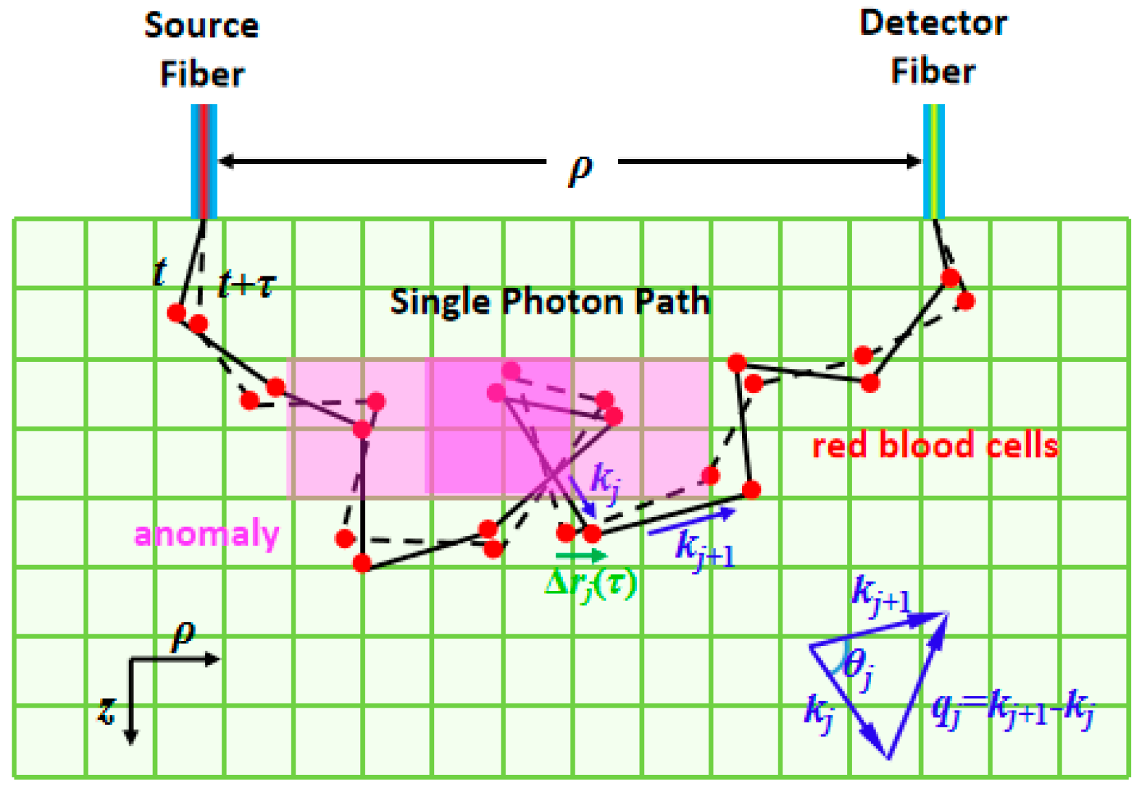
7]. Nevertheless, both Doppler ultrasound and laser Doppler measure the blood flow velocity along a specific major vessel wherein a dominant flow direction exists. At the microvasculature level, however, the red blood cells move diffusely in various directions. It is difficult for Doppler techniques to measure the velocity, because there is no dominant direction in the network of blood capillaries. By contrast, near-infrared diffuse correlation spectroscopy/tomography (DCS/DCT) quantifies the temporal autocorrelation function of light electric fields, which is sensitive to the Brownian motion of red blood cells in arbitrary directions. This motion is referred to as the blood flow index (BFI), with a unit of cm
2/s. The unit represents the spatial rate of blood flow dispersion per unit time, specifically applicable for evaluating microcirculation perfusion efficiency. Although the flow units of DCS/DCT and the Doppler technique are not directly comparable, the blood flow measurements by DCS/DCT have been widely validated in previous studies, evidenced by high correlations with routine flow modalities such as Doppler ultrasound [
8], laser Doppler [
9], and arterial spin labeling magnetic resonance imaging (ASL-MRI) [
10], as well as
15O-water PET [
11]. Moreover, previous reports [
11] have demonstrated that the blood flow index (BFI) can be thoroughly calibrated and converted to conventional absolute cerebral blood flow (CBF) units (mL/100 g/min). Another microscopic structural imaging technique is optical sectioning, which focuses on eliminating out-of-focus interference through optical methods to achieve high-resolution three-dimensional but superficial structural visualization [
12]. Recently, diffuse correlation spectroscopy/tomography (DCS/DCT) has been widely used to assess various diseases characterized by localized perfusion abnormalities, including neurological deficits (e.g., acute stroke, intracerebral hemorrhage, traumatic brain injury, and subarachnoid hemorrhage [
13,
14]), skeletal muscle disorders (e.g., myasthenia gravis, progressive muscular dystrophy, periodic paralysis, and burn injuries [
15,
16,
17]), and breast pathologies (e.g., tumors and hyperplasia [
18,
19]).
Compared with DCS, DCT enables spatial reconstruction of BFI distributions, providing critical advantages for tumor localization and morphological characterization (including size, shape, and position). Like other tomographic techniques, diffuse correlation tomography requires multiple source-detector pairs to acquire sufficient measurement data. However, due to practical constraints in instrumentation costs, the acquired data volume remains substantially smaller than the number of reconstruction voxels, resulting in severely ill-posed inverse problems in diffuse correlation tomography [
20,
21,
22,
23]. Traditional diffuse correlation tomography employs two primary algorithmic approaches: analytical methods and numerical analysis methods (NAMs). To address the inherent ill-posedness of the inverse problem, these algorithms incorporate various regularization techniques to improve BFI reconstruction quality. In analytical approaches, the inversion of correlation diffusion equations is typically achieved through singular value decomposition (SVD). The Tikhonov regularization parameter λ is optimally determined via
L-curve analysis [
22,
23]. However, analytical methods require the assumption of semi-infinite tissue geometry, which restricts their applicability for imaging highly curved brain surfaces or irregular tumor morphology. As a representative numerical approach, the finite element method (FEM) has been adapted from diffuse optical tomography (DOT) [
20] to diffuse correlation tomography (DCT) [
24,
25] to overcome these geometric and heterogeneity constraints. In this method, a modified Tikhonov minimization, equivalent to applying a Laplacian-type filter [
26], is used to minimize variation within each region. Nevertheless, current FEM implementations remain limitations because only a single data point from the normalized electric field autocorrelation function
g1(
τ) curve is utilized for BFI reconstruction, potentially introducing imaging errors.
To overcome the above-mentioned drawbacks, we previously [
21] developed an
Nth-order linearization (NL) algorithm that transforms the nonlinear correlation diffusion equation into a linear form through Taylor series expansion of
g1(
τ). This approach utilizes the slope of
g1(
τ) as projection data for BFI reconstruction, enabling adaptive selection of multiple data points for slope fitting to improve signal-to-noise ratio (SNR) based on noise characteristics. However, this method introduces three cumulative error sources: (1) Primary bias from linear regression during slope estimation of
g1(
τ); (2) An additional reconstruction error through iterative solutions of the ill-posed inverse problem using slope data; and (3) A systematic error in the Siegert relation when converting experimental
g2(
τ) measurements to
g1(
τ), where the coherence factor
β (typically ≈ 0.5 for single-mode fibers) introduces quantification inaccuracies. The error propagation originates from the fundamental measurement principle: diffuse correlation spectroscopy/tomography would generally reconstruct BFI values from intensity fluctuations of scattered light caused by moving red blood cells. This requires conversion of experimentally measured
g2(
τ) to
g1(
τ) via the Siegert relation, establishing a cascade of error accumulation throughout the reconstruction pipeline.
Deep learning, particularly large language models (LLMs), demonstrates universal approximation capabilities that enable direct nonlinear mapping from raw data to reconstructed images, especially in dynamic scattering media [
27]. By establishing an end-to-end mapping from
g2(
τ) measurements to BFI images, deep learning approaches could potentially bypass the three-stage error accumulation existing in conventional methods, meanwhile significantly reducing the computational time. However, two critical barriers currently impede this application: (1) The lack of standardized DCT datasets pairing
g2(
τ) data with corresponding BFI ground truth (GT); and (2) The absence of specialized neural network architectures optimized for DCT-based blood flow reconstruction. Recent advances in deep learning for DCS provide relevant methodological insights: Poon et al. [
28] implemented MobileNetV2 for BFI quantification in DCS; Feng et al. [
29] developed a ConvGRU network for direct temporal BFI prediction from
g2(
τ); and Zhang et al. [
30] employed support vector machines (SVMs) for
g1(
τ) denoising prior to BFI calculation. Recent advances have demonstrated the application of deep learning to DCT blood flow reconstruction. Notably, Liu et al. [
31] developed a hybrid architecture combining LSTM networks for
g1(
τ) curve denoising with convolutional neural networks (CNNs) for tomographic BFI image reconstruction. Li et al. [
32] proposed DCT-Unet, a U-Net variant with six-stage encoding, to leverage prior knowledge in establishing the
g1(
τ)-to-BFI mapping. While both approaches utilize
g1(
τ) data, they differ fundamentally in data utilization: Liu’s method processes only intermediate
g1(
τ) segments, while Li’s network incorporates nearly complete
g1(
τ) profiles. These methods are distinct from the traditional NL algorithms that are restricted to initial
g1(
τ) segments where Taylor series approximations remain valid (
τ→0). Nevertheless, three critical limitations persist: (1) Computational constraints prevent full
g1(
τ) waveform utilization due to memory-intensive training requirements; (2) Current implementations output either normalized or binarized blood flow values, deviating from absolute flow quantification; and (3) The inherent information loss during
g2(
τ)→
g1(
τ) conversion remains unaddressed.
Therefore, the core contributions of this work have three aspects: (1) Dataset construction: development of a comprehensive paired dataset containing g2(τ) measurements with corresponding BFI GT, incorporating fundamental characteristics of diffuse correlation spectroscopy; (2) Network architecture: implementation of Conv-TransNet, a novel hybrid CNN–Transformer model capable of direct end-to-end mapping from initial g2(τ) segments to BFI tomographic images; and (3) Experimental validation: computational simulations using tissue models with varying anomaly configurations (morphology, spatial distribution, dimensions), phantom studies under controlled conditions, and comparative performance analysis against conventional CNN architectures and NL algorithms.
3. Conv-TransNet Model
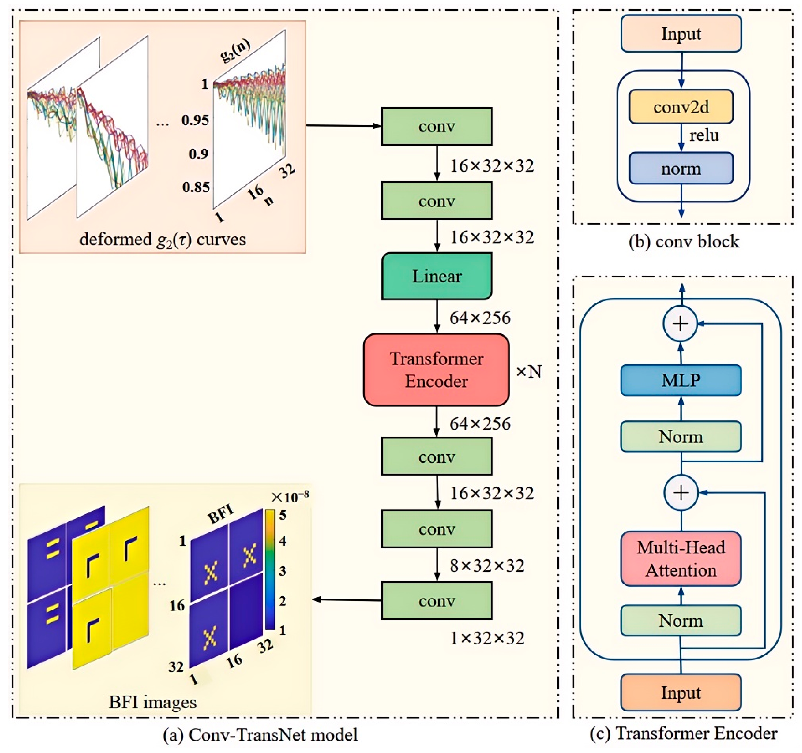
In this study, we adapt a hybrid Conv-TransNet architecture (integrating CNN and Transformer modules) for diffuse correlation tomography applications. The complete network architecture is illustrated in
Figure 5.
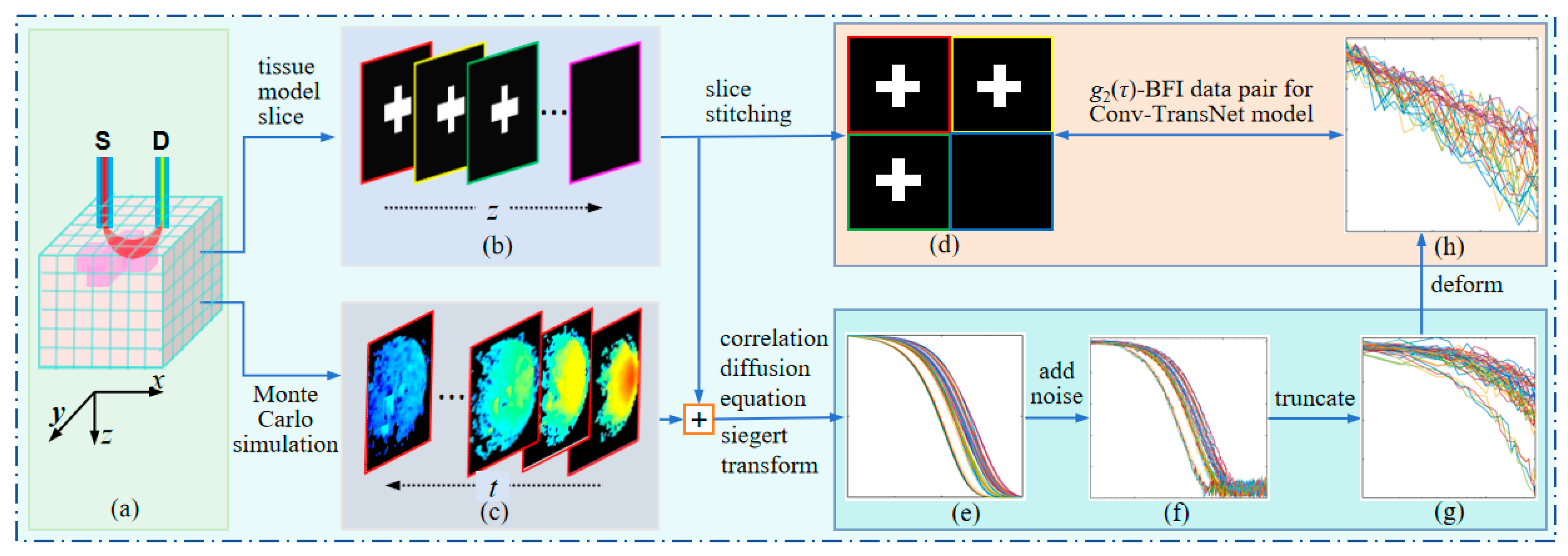
As previously described, the truncated and reshaped
g2(
τ) matrix serves as the input to the convolutional block (conv,
Figure 5a). This block comprises three key components: a 2D convolutional (conv2d) layer, ReLU activation function, and normalization layer (norm layer), which collectively extract shallow features from the processed
g2(
τ) curves. The extracted features are then passed through a fully connected layer, where the 32 × 32
g2(
τ) matrix undergoes linear transformation into a 64 × 256 matrix. This expanded matrix is subsequently processed by the Transformer Encoder (
Figure 5b), which contains two core components: multi-head attention (MHA) and a multi-layer perceptron (MLP).
The encoder employs MHA to capture correlations among sequence elements, and the MLP is adopted to perform nonlinear transformations. This architecture enables the network to learn higher-level feature representations. To enhance generalization and mitigate gradient vanishing/exploding issues, residual connections are incorporated throughout the encoder. Finally, the decoder reconstructs a 32 × 32 blood flow image through three conv. The key design elements include (1) the norm layer to accelerate convergence and prevent overfitting; (2) the ReLU activation functions to enhance nonlinear modeling capacity; and (3) the uniform convolutional parameters: stride = 1, kernel_size = 3 with padding maintained at all Conv2D layers.
As shown in
Figure 5a, the structure of our Conv-TransNet model demonstrates that the input truncated and reshaped
g2(
τ) are first compressed into a low-dimensional space, then ultimately mapped to the image domain through feature extraction and fusion. This process involves five convolutional blocks, one linear layer, and nine encoder layers. In essence, the model establishes a direct end-to-end mapping between the input
g2(
τ) data and the output four-slice spliced blood flow images. The proposed method significantly improves the speed of blood flow reconstruction, meanwhile enhancing its intuitiveness.
During training, we adopt the Huber loss as the loss function, with a learning rate of 7 × 10⁻⁵. The model is trained for 300 epochs with a batch size of 4 and optimized by using Adam. The implementation is based on Python (version 3.12) and PyTorch (version 2.6.0), running on an Intel Core i7-6700MQ CPU and an NVIDIA GTX 3080 Ti GPU.
For the CNN architecture, we design seven convolutional blocks, three residual layers, one concatenation layer, and six convolutional layers for feature extraction and fusion. The implementation also employs the Huber loss function and Adam optimizer, with the remaining hyperparameters consistent with the original Conv-TransNet configuration.
4. Evaluation Criteria and Experiments Results
In this study, comprehensive simulations and phantom experiments were designed to rigorously evaluate the performance of the proposed Conv-TransNet model for diffuse correlation tomography. For simulations, five heterogeneous tissue models with distinct anomaly geometries were tested: a two-dot anomaly (case A), asymmetric cross-shaped anomaly (case B), rectangular anomaly (case C), Z-shaped anomaly (case D), and two-bar anomaly (case E). For the phantom experiments, two physiologically relevant scenarios were investigated: a quasi-solid cross-shaped anomaly (case F) and the speed-varied liquid tubular anomalies (case G, H, I). The results of the Conv-TransNet model, CNN, and NL algorithm will be shown in this part, along with the evaluation criteria.
4.1. Evaluation Criteria
To comprehensively evaluate the performance of Conv-TransNet, we conducted comparative experiments with the CNN and NL algorithm, assessing both visual reconstruction quality and quantitative metrics.
Root mean squared error (RMSE) quantifies the difference between the reconstructed and the true images, and it is defined as follows:
Here, and are the reconstructed and true blood flow index of the ith tissue voxel, respectively. A smaller RMSE value indicates that the reconstructed blood flow index image is closer to the true one.
CONTRAST quantifies the difference between the anomalies and background, which is defined as follows.
Here, αDB-anomaly is the average reconstructed BFI of the anomalous voxels, and αDB-background is the average BFI of the background. Under conditions (anomaly blood flow index = 5 × 10⁻⁸ cm2/s, background = 1 × 10⁻⁸ cm2/s), the theoretical maximum CONTRAST value of 5 indicates perfect reconstruction fidelity.
Furthermore, the misjudgment ratio (MJR) was defined by us to evaluate the performance of the three methods.
Here, the false-positive rate (FPR) refers to the probability of normal voxels being misjudged as anomalies; for instance, in scenarios with anomalies of 5 × 10⁻⁸ cm2/s against backgrounds of 1 × 10⁻⁸ cm2/s, normal voxels will be flagged as anomalous when exceeding the entire volume mean BFI by 20% (1.2 × 10⁻⁸ cm2/s). The false negative rate (FNR) is the probability that an anomaly (beyond 20% of the global average) is incorrectly labeled as normal.
4.2. Computer Simulation with Noisy Data
Figure 6 displays the reconstructed splicing blood flow index images derived from noisy
g2(
τ) data. The first column (A1, B1, C1, D1, and E1) shows the ground truth (GT) tissue models for five types of anomalies: two-dot anomaly (first three slices, 2 voxels per slice), asymmetric cross-shaped anomaly (first three slices, 8 voxels per slice), rectangular anomaly (first three slices, 8 voxels per slice), Z-shaped anomaly (first three slices, 8 voxels per slice), and two-bar anomaly (first three slices, 6 voxels per slice). The background is 1 × 10
−8 cm
2/s, while anomalies have a BFI of 5 × 10
−8 cm
2/s. The second column (A2, B2, C2, D2, and E2) shows the reconstructed blood flow index images by the Conv-TransNet model for the five types of anomalies, respectively. The third column (A3, B3, C3, D3, and E3) displays the reconstructed images by the CNN for the same five anomalous types. The fourth column (A4, B4, C4, D4, and E4) depicts the images reconstructed by the NL algorithm. From the figures, we observe that all three methods accurately reconstruct the spatial locations of the anomalies. However, in terms of shape and size fidelity, the Conv-TransNet model and CNN yield more regular and GT-like reconstructions when compared with the NL algorithm. Specifically, the Conv-TransNet model achieves more accurate reconstruction of both the rectangular (
Figure 6(C2)) and Z-shaped anomalies (
Figure 6(D2)), precisely matching their true morphology and dimensions without introducing peripheral artifacts. By comparison, while the CNN method similarly reconstructs the correct shape and size of these anomalies, it generates a single false-positive voxel in each of the asymmetric cross-shaped and rectangular anomalous regions and three false-positive voxels in Z-shaped and two-bar anomalies. An additional advantage of the Conv-TransNet model and CNN is their consistent reconstruction quality regardless of anomaly depth. By contrast, the performance of the NL algorithm deteriorates progressively with depth, with nearly complete failure to recover anomalous blood flow index in the third layer.
For quantitative evaluation, the RMSE, CONTRAST, and MJR are listed in
Table 1. As shown in it, the Conv-TransNet model achieves significantly lower RMSE values for all five types of anomalies compared to both the CNN and NL algorithms. Specifically, for the rectangular anomaly, the RMSE of the NL algorithm (13.62%) and CNN (9.32%) are approximately 6.33 and 4.33 times higher than that of the Conv-TransNet model (2.15%), respectively. This demonstrates that the Conv-TransNet model’s reconstruction achieves superior fidelity to the GT.
CONTRAST and MJR metrics were calculated based on the first two slices, as the performance of the NL algorithm degrades significantly in the third slice. The CONTRAST metrics of the five different anomalies reconstructed by Conv-TransNet model are 5.13, 4.39, 4.62, 4.13, and 4.20, respectively. Although the CONTRAST metrics for cross-shaped and rectangular anomalies are slightly lower than those obtained by CNN (4.67 and 4.92, respectively), they remain close to the theoretical optimum of 5 (background: 1 × 10⁻⁸ cm2/s; anomaly: 5 × 10⁻⁸ cm2/s) and are significantly superior to the results of the NL algorithm.
For the MJR metric, the Conv-TransNet model achieved almost 0% values across all five types of anomalies. Both the CNN and NL methods showed 0% MJR for the two-dot anomaly. However, for the cross-shaped anomaly, the CNN showed 0.39% MJR, primarily due to FPR (2 false-positive voxels/512 voxels in the first two slices), and the NL algorithm exhibited 2.34% MJR, also FPR-dominated. Similarly, for rectangular anomalies, the CNN maintained 0.39% MJR, and the NL algorithm demonstrated 4.69% MJR, with both cases being predominantly FPR. For the Z-shaped and two-bar anomalies, only one false-positive voxel was identified, corresponding to a 0.19% MJR. These rates are substantially lower than those achieved by the CNN and NL methods.
To investigate whether the truncating and reshaping
g2(τ) curves would cause data loss and whether longer truncation would improve results or not, we analyzed cases C (rectangular anomaly) and D (two-bar anomaly). Specifically, (1) We truncated each of the 48
g2(τ) curves to 30 initial data points and reshaped them into a 38 × 38 matrix; (2) We alternatively used the first 48 data points from all 48 curves to directly construct a 48 × 48 matrix without reshaping. The reconstructed images for three different delay times are shown in
Figure 7. The first row of
Figure 7 presents reconstructed images of case C (rectangular anomaly), with (a) GT and (b)–(d) displaying reconstructions using 22, 30, and 48 delay-time points, respectively. The second row shows case F (two-bar anomaly), where (e) presents the GT, while (f)–(h) demonstrate reconstructions by using 22, 30, and 48 delay-time points, respectively. The results clearly demonstrate that reconstruction quality deteriorates as the delay time τ increases. Notably, the reconstruction with 48 delay-time points shows severe distortion.
Quantitative analysis in
Table 2 further confirms this trend, showing that reconstruction quality worsens with the increasing delay-time points. For the two-bar anomaly, the RMSE increases from 4.39 to 15.93, while the contrast decreases from 4.24 to 3.87. Potential reasons for these observations will be discussed in the Discussion section.
4.3. Phantom Experiment
4.3.1. The Quasi-Solid Cross-Shaped Anomalous BFI Phantom Experiment
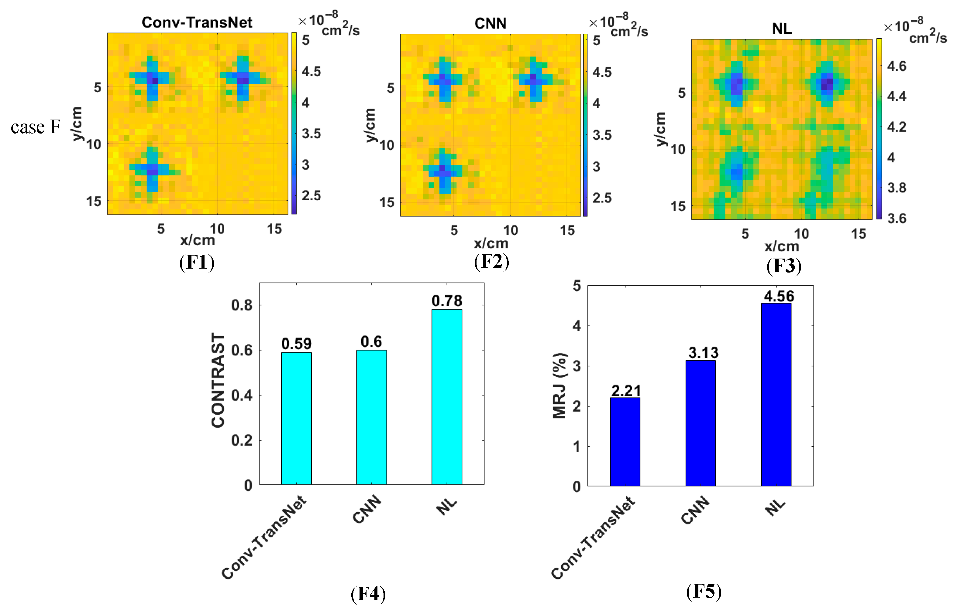
Figure 8 presents the reconstruction results of the quasi-solid cross-shaped anomaly (Case F) phantom experiment, with panels (F1), (F2), and (F3) showing the outputs from the Conv-TransNet model, CNN, and NL algorithm, respectively. Figure analysis reveals that all three methods can clearly resolve both the spatial location and morphological characteristics of the quasi-solid cross-shaped anomalies. Comparative analysis demonstrates that both Conv-TransNet and the CNN yield more regular morphological features and significantly fewer artifacts than the NL algorithm. Furthermore, quantitative evaluation reveals that the Conv-TransNet reconstruction contains marginally fewer artifacts compared to the CNN results.
For quantitative evaluation in the phantom experiments where ground truth (GT) data were unavailable, CONTRAST and MJR served as the primary metrics for comparing the performance of the three methods. As shown in
Figure 8(F4), the CONTRAST values of the first three slices are 0.59, 0.60, and 0.78 for the Conv-TransNet model, CNN and NL algorithm, respectively. Although both deep learning methods achieved nearly identical CONTRAST values, the Conv-TransNet model demonstrated significantly lower MJR (2.21% vs. CNN: 3.13%;
Figure 8(F5)) under our revised FPR criterion. Here, FPR was redefined to classify normal voxels as false positives when their BFI is 10% lower than the entire solution—a criterion accounting for the inherently lower BFI of the quasi-solid anomaly. Error analysis confirmed that misjudgments are predominantly false positives in both cases. The NL algorithm yielded a substantially higher MJR of 4.56%, with error decomposition demonstrating this was predominantly FNR—a clinically significant drawback that may lead to missed diagnoses in practical applications.
4.3.2. The Speed-Varied Liquid Tubular Anomaly Phantom Experiment
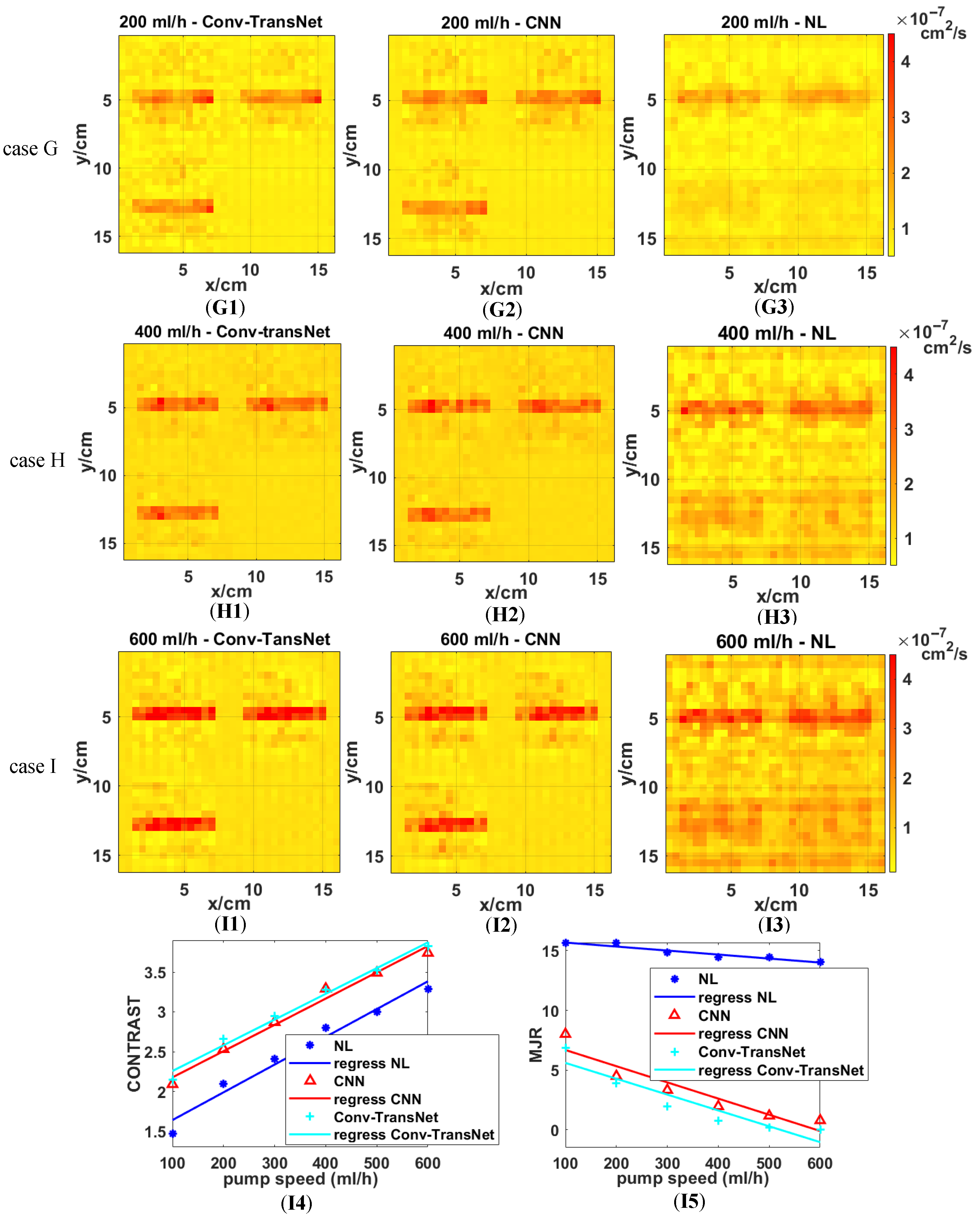
All three methods were evaluated on tubular anomalies at the varied flow velocities (100–600 mL/h, 100 mL/h increments). Representative reconstructions for 200 mL/h (Case G), 400 mL/h (Case H), and 600 mL/h (Case K) are displayed in
Figure 9, as well as the quantitative metrics (CONTRAST and MJR) from the first two slices.
Figure 9 demonstrates the superior performance of deep learning methods, with Conv-TransNet (G1, H1, I1) and CNN (G2, H2, I2) producing more uniform backgrounds and sharper tubular anomaly contours compared to the NL algorithm (G3, H3, I3). Notably, both deep learning methods maintain consistent anomaly detection, even at low flow rates (200 mL/h) and across varying depths, meanwhile avoiding the performance degradation observed in NL algorithm results.
Figure 9 further demonstrates that while deep learning methods enhance reconstruction quality for high-flow-rate tubular anomalies (e.g., 600 mL/h), the Conv-TransNet model particularly excels in low-flow-rate conditions (200 mL/h), yielding more discernible anomaly delineation compared to conventional approaches.
Figure 9(I4) demonstrates a flow-rate-dependent increase in CONTRAST for all methods, with particularly significant improvements at lower flow velocities. The Conv-TransNet model achieves a 46.3% higher CONTRAST (2.15 vs. 1.47) at 100 mL/h than the NL algorithm. This improvement gradually stabilizes across higher flow rates (200–600 mL/h), showing consistent increments of 0.56, 0.53, 0.43, 0.50, and 0.53, respectively, with a mean improvement of 0.55 ± 0.06 across all tested flow rates. Regarding MJR, as shown in
Figure 9(I5), the NL algorithm maintains approximately 15%, with only marginal improvement as flow velocity increases. By contrast, the deep learning methods achieve much lower MJR values (close to zero) with the increasing flow rates. These results provide further evidence of deep learning’s superior performance over conventional NL algorithms.
Quantitative comparison reveals that while the Conv-TransNet model achieves marginally higher CONTRAST values than CNN, it demonstrates substantially superior MJR performance. As evidenced in
Figure 9(I5), (1) at the 100 mL/h flow rate, Conv-TransNet attains 6.84% MJR versus CNN’s 8.01% (14.6% relative improvement); (2) at 600 mL/h, Conv-TransNet reaches perfect 0% MJR compared to CNN’s residual 0.78% error rate.
5. Discussion
This work proposes a CNN–Transformer model for direct mapping of g2(τ) data to BFI images, outperforming conventional approaches. However, the novel insights and reconstruction challenges identified warrant further in-depth analysis.
The primary advantage of the Conv-TransNet model is its ability to directly process the
g2(
τ) data matrix as the input without complex preprocessing or manual feature extraction, achieved through a self-attention mechanism that models inter-element dependencies via pairwise correlation calculations [
38]. Furthermore, to optimize computational efficiency and reduce storage demands, the raw
g2(
τ) curves are truncated and resampled. As illustrated in
Figure 2h and
Figure 5a, the truncated
g2(
τ) is transformed into a discrete representation, denoted as
g2(
n). Here, the x- and y-axes solely represent discrete data points, decoupled from the original correlation time
τ.
Certainly, the proposed Conv-TransNet model also has limitations. For instance, the CONTRAST values for cross-shaped (4.62) and rectangular (4.13) anomalies are slightly lower than those achieved by the CNN (4.67 and 4.62, respectively). This performance gap may stem from the reliance of transformer architectures on large-scale datasets. Although we constructed 18,000 noise-free and noisy data pairs, these were essentially generated through positional variations of merely ~100 distinct anomaly prototypes, lacking true sample independence. In such small-sample, strongly ill-posed, and noise-corrupted inverse tasks, CNNs often demonstrate superior practical value due to their local inductive bias (spatial priors) and parameter efficiency. Conversely, when training data is insufficient or the architecture is not fully optimized for the physical model, hybrid designs may inadvertently compromise sensitivity to subtle hemodynamic variations.
In computer simulations, anomalies with varying BFI values were randomly selected for testing, yet all coincidentally exhibit higher BFI than the background (
Figure 6). The speed-varied liquid tubular anomalies also have higher BFI. The high BFI anomaly is used to mimic hyperperfusion states induced by malignant tumors, neural activation, or high-intensity exercise. By contrast, the quasi-solid cross-shaped anomaly with lower blood flow than the surrounding medium (
Figure 8) is designed to simulate clinical scenarios of hypoperfusion caused by calcified tissues or ischemia. It is important to note that DCS/DCT detects Brownian motion of particles rather than direct flow velocity [
34]. The cross-shaped anomaly is a quasi-solid, and its Brownian motion is attenuated yet persists—albeit weaker than the background liquid solution. Thus, its expected CONTRAST should be less than 1. The Conv-TransNet model produces a CONTRAST of 0.59, significantly lower than that of the NL algorithm (0.77). This indicates its higher accuracy in modeling the physical characteristics of the anomaly, where the quasi-solid state attenuates Brownian motion.
Another challenge lies in the complexity of anomalies. As shown in
Table 1, the RMSE increases with anomaly complexity. The two-dot anomaly represents the simplest case, consistently yielding the lowest RMSE across all three methods. The asymmetric cross-shaped, rectangular, and Z-shape anomalies all occupy 8 voxels in the first three slices. On the other hand, however, the asymmetric cross-shaped and Z-shape anomalies exhibit higher RMSE values (4.43 and 4.05) than the rectangular anomaly (2.15). This discrepancy stems from the cross-shaped anomaly’s higher curvature.
In
Figure 7 and
Table 2, we validate the influence of correlation delay time on the quality of reconstructed images, revealing superior anomaly reconstruction with shorter delays. The underlying reason may be explained by the principle of DCT: specifically, initial shorter correlation time
τ corresponds to stronger correlation, and even a slight delay time can lead to a rapid decrease in
g2(
τ). Conversely, the latter longer
τ exhibits weaker correlation, resulting in gradual
g2(
τ) decay. Consequently, data acquired with the latter large delay time are less conducive to the model’s extraction of data features, which in turn impairs the reconstruction quality. This fundamental principle is the basis of both the NL algorithm [
21] and FEM [
26], where shorter delay times (
τ ∈ [10
−7, 2.7 × 10
−6] s) are selected to optimize reconstruction accuracy.
In phantom experiments, the definitions of FNR and FPR are different due to the different BFI of the two kinds of anomalies, but their assessment logic is unified. For Conv-TransNet model and the CNN, FPR is mainly MJR, whereby FNR is dominant MJR for the NL algorithm. However, false negatives pose significant clinical risks for tumor detection and treatment. This limitation stems from the ill-posed linear equations and back-projection initial values used by the NL algorithm, which inevitably lead to homogenized reconstructed images [
36].
Furthermore, as shown in
Figure 9, while deep learning methods enhance reconstruction quality for tubular anomalies at both lower and higher flow velocities, they show limited improvement for intermediate flow rates. For instance, the CONTRAST obtained by the Conv-TransNet model is increased by 0.68, 0.56, 0.53, 0.43, 0.50, and 0.53 at flow rates of 100–600 mL/h (in 100 mL/h increments), respectively. This phenomenon may be attributed to the imbalanced distribution of training data, which is predominantly categorized into two extremes: 1 × 10
−8 cm
2/s and 5 × 10
−8 cm
2/s. Such data distribution enhances contrast sensitivity at low flow velocities while better accommodating high flow rate conditions but appears to compromise performance at intermediate ranges.
