Learnable Priors Support Reconstruction in Diffuse Optical Tomography

Abstract

Diffuse Optical Tomography (DOT) is a non-invasive medical imaging technique that makes use of Near-Infrared (NIR) light to recover the spatial distribution of optical coefficients in biological tissues for diagnostic purposes. Due to the intense scattering of light within tissues, the reconstruction process inherent to DOT is severely ill-posed. In this paper, we propose to tackle the ill-conditioning by learning a prior over the solution space using an autoencoder-type neural network. Specifically, the decoder part of the autoencoder is used as a generative model. It maps a latent code to estimated physical parameters given in input to the forward model. The latent code is itself the result of an optimization loop which minimizes the discrepancy of the solution computed by the forward model with available observations. The structure and interpretability of the latent space are enhanced by minimizing the rank of its covariance matrix, thereby promoting more effective utilization of its information-carrying capacity. The deep learning-based prior significantly enhances reconstruction capabilities in this challenging domain, demonstrating the potential of integrating advanced neural network techniques into DOT.

1. Introduction

In recent years, Diffuse Optical Tomography (DOT) has shown potential as a medical diagnostic imaging modality suitable for screening and therapeutical follow up [1]. Differently from X-ray based CT, DOT uses near-infrared (NIR) light as an investigating signal. In this spectral window, light can penetrate for several centimeters into biological soft tissues, providing optical access to information on tissue chromophores such as oxy-hemoglobin (HbO₂), deoxy-hemoglobin (Hb), lipids, and water (H₂O), which represent relevant biomarkers of cancer, stroke, and other tissue diseases [2,3]. In this work, we focus on DOT based on continuous waves (CW) systems, which are among the most widely used in clinical screening applications such as breast cancer diagnosis. A typical CW-DOT imaging device is composed of an array of emitters (low-power LEDs or lasers) and detectors which measure at various locations on the surface of the tissue [4] the transmitted or reflected light beamed into the tissue. Due to the mixture of coherent, quasi-coherent, and predominant non-coherent NIR wavelength photons as well as limited valid boundary measurements, the reconstruction of tissue optical properties in Diffuse Optical Tomography is a notoriously severely ill-posed and ill-conditioned inverse problem; therefore, regularization techniques providing hard or soft priors are essential to obtain a trustworthy solution [5,6]. In the past, DOT reconstruction has been based on model-driven algorithms, whose design follows directly from the underlying mathematical problem formulation [7]. To address the ill-conditioning, these solvers include regularizations typically based on ${\ell }_2$-norm (Tikhonov/ridge regression) penalization and/or ${\ell }_1$-norm (lasso) penalization [8,9,10], or a convex combination of these norms by Elastic Net regularization [11]. Other approaches replace the regularization functional with its Bregman distance [12]. Although these procedures have been proven to recover the solution of the inverse problem in selected cases, the tuning of model regularization parameters and computational complexity remain very critical. In addition, complex distributions of the optical coefficients remain very hard to reconstruct.

Recent advances in deep learning have prompted a paradigm shift in tomographic imaging research, moving from solely knowledge-driven methodologies to predominantly data-driven approaches. Nowadays, these approaches are consistently applied to a variety of medical imaging modalities, including computed tomography (CT) [13] and MRI [14], but their application in DOT reconstruction is still in its infancy. Patra et al. [15] used an embryonic version of a fully connected NN with two hidden layers to obtain a prior on the spatial localization of a single contrast region embedded in a 2D circular domain. Accordingly, in the iterative reconstruction procedure, they updated only the parameters in a neighborhood around the detected contrast region. Sun et al. [16] addressed the multiple scattering problem of microwaves in biological samples using a two-step reconstruction method, where an analytical method based on the linear backprojection operator provided a first image estimate, followed by a U-Net decoder for image reconstruction. This approach avoided the iterative evaluation of the nonlinear discrete Lippmann–Schwinger operator (or its Jacobian). Feng et al. [17] adopted a NN based on a fully connected architecture made of three layers for end-to-end DOT image reconstruction, the internal hidden layer comprising 695 neurons, for a total of about 1.56 M parameters in the test examples. Fully data-driven approaches, which completely rely on data and do not assume the existence of a physical model of the underlying processes, have become a relevant part of new research in this field. Yoo et al. [18] investigated an end-to-end model based on a DNN architecture to reconstruct heterogeneous optical maps in small animals. A fully connected layer performed a first inversion, followed by an encoder–decoder structure which implemented a deep 3D convolutional framelet. Deng et al. [19] proposed an architecture in which a fully connected layer input the data into an encoder–decoder structure followed by a U-Net for image denoising and quality improvement. Skip connections further enhanced high-resolution features for reconstruction. Mozumder et al. [20] combined deep learning and model-based approaches in the so-called Deep Gauss-Newton architecture that uses the Gauss Newton algorithm to solve the DOT inverse problem, where the update function is learned via a convolutional neural network. In [21], some of the authors of the present work proposed a fully data-driven approach for DOT, called Mod-DOT neural architecture, where two different autoencoders separately process data and originating signal, and a “bridge” network connects the two latent spaces and acts as a learned regularizer.

In this work, we propose a novel hybrid knowledge and data-driven framework to address the DOT inverse problem, leveraging a generative model as learnable prior to characterize the manifold of plausible optical parameters. The introduction of a sequence of linear layers between the encoder and the decoder encourages the autoencoder to learn a low-rank latent space, providing an effective low-dimensional representation of the data. Our approach also integrates the resolution of the forward problem via a Graph Neural Network into the iterative reconstruction process [22]. This implies that at each iteration of the optimization problem, new physical insights from the forward problem are incorporated, allowing the network to act as a learned model correction mechanism, compensating for the wrong components of the latent space and extracting relevant information to guide the updates. The idea of combining a learned forward solver—such as a Graph Neural Network or Fourier Neural Operator—with a learned prior has been previously explored in the context of PDE-based inverse problems [23,24]. However, to the best of our knowledge, this work represents the first application of such an approach to DOT reconstruction.

2. Materials and Methods

2.1. General Setting

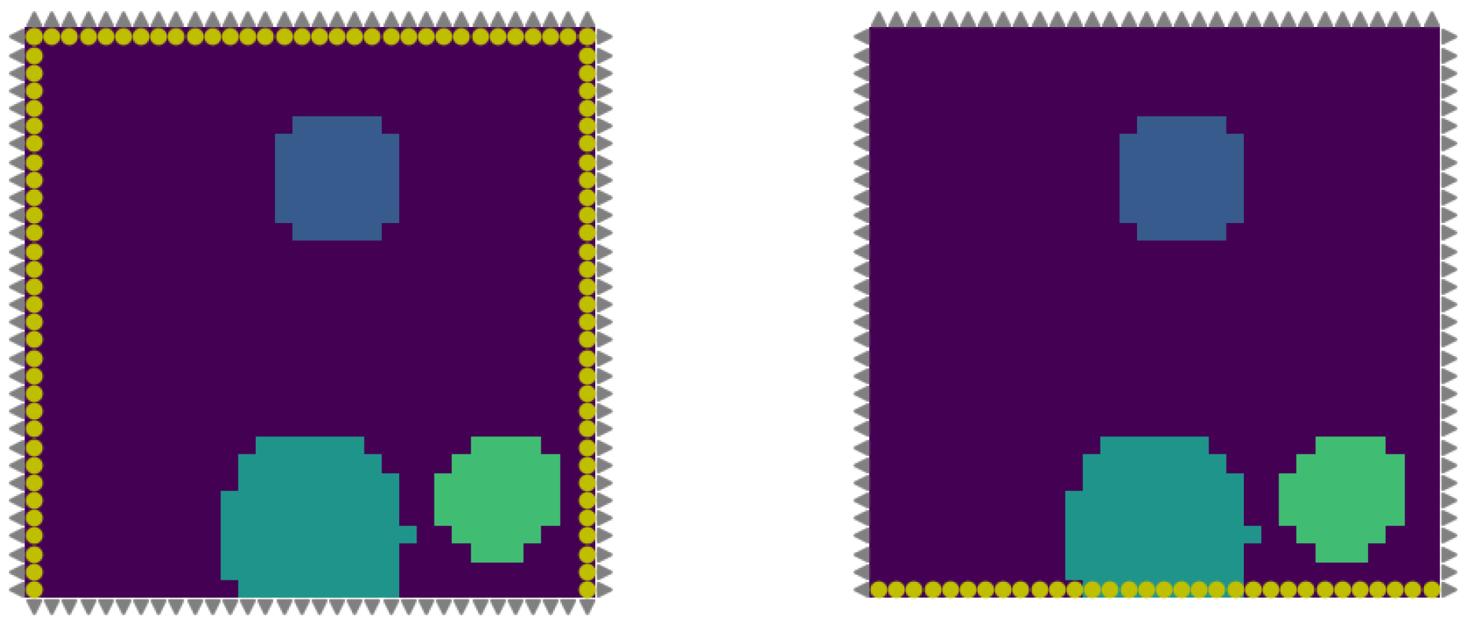
Let $\mathsf{\Omega }\subseteq {\mathbb{R}}^d$, $d=2,3$, be a bounded domain with boundary $\partial \mathsf{\Omega }$, representing the sample of biological tissue under investigation. Given the generic Banach spaces $Q,W$, and U of all admissible optical parameters, source terms, and light field, respectively, we denote by ${\mu }_a\in Q$ the spatially dependent optical parameters and by $u\in U$ the state variable representing the light fluence relating to a particular light source $f=f\left(x\right)\in W$, located at position $x\in \mathsf{\Omega }$. The light field u is the solution of the following PDE problem [11]:

$$\begin{array}{cc}\mathcal{L}(u;{\mu }_a)=f\hfill & \mathrm{in}\mathsf{\Omega },\hfill \\ \mathcal{B}\left(u\right)=0\hfill & \mathrm{in}\partial \mathsf{\Omega },\hfill \end{array}$$

(1)

where $\mathcal{L}:D\left(\mathcal{L}\right)\subset U\times Q\to W$ is an integro-differential operator endowed with generic boundary conditions given by the operator $\mathcal{B}$ that guarantee the well-posedness of Problem (1). By introducing the observation operator P which provides the solution field at the observations points, and the parameter-to-state map $S:D\left(S\right)\subseteq Q\to U$, i.e., $S\left({\mu }_a\right)=u$, which is a solution to the boundary value problem (1), we can define the forward map as $\mathcal{F}=P\circ S:D\left(S\right)\subseteq Q\to Y$, where Y is the Banach space of the measured light field at the detectors. The inverse problem of identification of optical parameters in DOT can be formulated as the optimization problem: seek the optimal ${\mu }_a^{\ast }$ such that

$${\mu }_a^{\ast }=\underset{{\mu }_a\in Q}{arg\; min}\mathcal{D}(\mathcal{F}\left({\mu }_a\right),y_{\delta }),$$

(2)

where $\mathcal{D}:Y\to [0,+\infty )$ is a discrepancy or loss function and $y_{\delta }$ is the noisy measurement vector for some noise level $\delta \ge 0$ obtained via the measurement map $\mathcal{M}:D\left(\mathcal{M}\right)\subset (Q\times U)\to Y$ such that $\mathcal{M}({\mu }_a;u)=y_{\delta }$ represents the measured light field at the observation points.

2.2. Forward Model

In the DOT framework, the parameter-to-state map arises from an underlying mathematical model, describing the light propagation in biological tissue. A model of this nature, both physically plausible and computationally efficient, is derived by expanding the Radiative Transfer Equation (RTE) in spherical harmonics and truncating the series at the first order [25], yielding the following PDE model, known as Diffusion Approximation (DA):

$$-\nabla ·(D\left(x\right)\nabla \left(u\left(x\right)\right))+{\mu }_a\left(x\right)u\left(x\right)=f\left(x\right),x\in \mathsf{\Omega },$$

(3)

where the field $u\left(x\right)={\int }_{S^{d-1}}I(x,s^{\prime })d{s}^{\prime }$ is the photon fluence due to the light source $f\left(x\right)$ and where $D=D\left(x\right)$ is the diffusion coefficient given by

$$D\left(x\right)={\displaystyle \frac{1}{d({\mu }_a\left(x\right)+(1-g){\mu }_s)}},$$

(4)

with g anisotropic scattering factor depending on the specific tissue and ${\mu }_s$ known scattering coefficient. The quantity ${\mu }_s^{\prime }=(1-g){\mu }_s$ represents the reduced scattering coefficient. Model (3) is equipped with the Robin-type boundary condition [25,26]

$$u\left(x\right)+{\displaystyle \frac{\zeta D\left(x\right)}{2c_d}}\nabla u\left(x\right)·n=0,x\in \partial \mathsf{\Omega },$$

(5)

which describes the interaction of light at the interface between biological tissue and surrounding media such as air or other materials, where $\zeta =(1+R)/(1-R)$, R being the reflection coefficient derived from the Fresnel’s law to account for the index mismatch between tissue and air, and where $c_d$ is the accommodation coefficient at the tissue–air interface which depends on the space dimension ($c_d=1/\pi$ if $d=2$, $c_d=1/4$ if $d=3$).

Using the method of Green’s function [27], we can express the solution of Problem (3) as the convolution between the source term f and the Green’s function $G(x,x^{\prime })$ for the modified Helmholtz operator

$$u\left(x\right)={\int }_{\mathsf{\Omega }}G(x,x^{\prime })f\left(x^{\prime }\right)d{x}^{\prime },$$

(6)

where $G:\mathsf{\Omega }\times \mathsf{\Omega }\to \mathbb{R}$ solves the following boundary value problem:

$$\left\{\begin{array}{cc}[\Delta -k^2]G(x,x^{\prime })=\delta \left(x^{\prime }\right)\hfill & x\in \mathsf{\Omega },\hfill \\ G(x,x^{\prime })+{\displaystyle \frac{\zeta D\left(x\right)}{2c_d}}\nabla G(x,x^{\prime })·n=0\hfill & x\in \partial \mathsf{\Omega },\hfill \end{array}\right.$$

(7)

where $\delta \left(x^{\prime }\right)$ is the Dirac delta distribution centered at $x^{\prime }$ and $k\left(x\right)=\sqrt{{\displaystyle \frac{{\mu }_a\left(x\right)}{D\left(x\right)}}}$ is the wave-number.

Graph Neural Network Solvers

Traditional methods for finding Green’s functions imply to derive analytical formulas, compute eigenvalue expansions, or numerically solve a singular PDE [27,28]. In this work, we leverage instead Neural Operators to learn the Green’s function directly from data. We construct a graph over the domain $\mathsf{\Omega }$ of the PDE such that the state variable is described as $u=(V;E)$, where V and E are the sets of graph nodes and edges, respectively. To establish the graph, we consider on the domain a uniform mesh where each node corresponds to the centroid of a voxel element and we choose the edge connectivity according to the Lebesgue measure. We model the forward operator $\mathcal{F}$ via a Graph Neural Network [29,30] where we encode the vector connecting the nodes x and y, along with its norm, as edge features $e(x,y)\in {\mathbb{R}}^{n_e}$. The quantities characterizing the state of the PDE are provided as node features $v_t\left(x\right)\in {\mathbb{R}}^n$, with n dimension of representation. Namely, we have

$$\begin{array}{c}{\mathcal{G}}_{\theta }:Q\to U,\hfill \\ {\mathcal{G}}_{\theta }:=\mathcal{Q}\circ {\sigma }_T(W_{T-1}+{\mathcal{K}}_{T-1})\circ \dots \circ {\sigma }_1(W_0+{\mathcal{K}}_0)\circ \mathcal{P},\hfill \end{array}$$

(8)

with the following architecture:

• Lifting layer: The input states are lifted to some higher dimensional space using multi-layer perceptrons (MLPs) as follows:

  $$v_0=\mathcal{P}(x,{\mu }_a\left(x\right))$$

  (9)
• Kernel integration layer: The processing step consists of several message passing layers with residual connections:

  $$v_{t+1}\left(x\right)={\sigma }_{t+1}\left(W_t{v}_t\left(x\right)+\underset{:={\mathcal{K}}_t\left(v_t\left(x\right)\right)}{\underbrace{{\int }_{\mathsf{\Omega }}{\kappa }_{\varphi }^{\left(t\right)}(x,y,{\mu }_a\left(x\right),{\mu }_a\left(y\right))v_t\left(y\right)dy}}\right),t=0,\dots ,T-1$$

  (10)

  where ${\sigma }_{t+1}:\mathbb{R}\to \mathbb{R}$ is an activation function applied element-wise, $W_t\in {\mathbb{R}}^{n\times n}$ is a tunable tensor, and ${\kappa }_{\varphi }$ is a tensor kernel function that is modeled by a Neural Network with learnable parameters $\varphi$.
• Projection layer: In the final decoding step, an MLP transforms the latent node features $v_T\left(x\right)$ into the output features $u\left(x\right)$:

$$u\left(x\right)=\mathcal{Q}{v}_T\left(x\right)$$

(11)

We train the Graph Neural Network with respect to the mean squared error (MSE):

$${\theta }^{\ast }=\underset{\theta }{argmin}\sum _i\sum _{x\in \mathsf{\Omega }}{\parallel u_{gt}^i\left(x\right)-\mathcal{G}({\mu }_a^i;\theta )\left(x\right)\parallel }_2^2$$

(12)

where $\theta$ is the collection of the network parameters for the Graph Neural Network and $u_{gt}^i$ is the ground truth light field for each $i-$th sample in the training set.

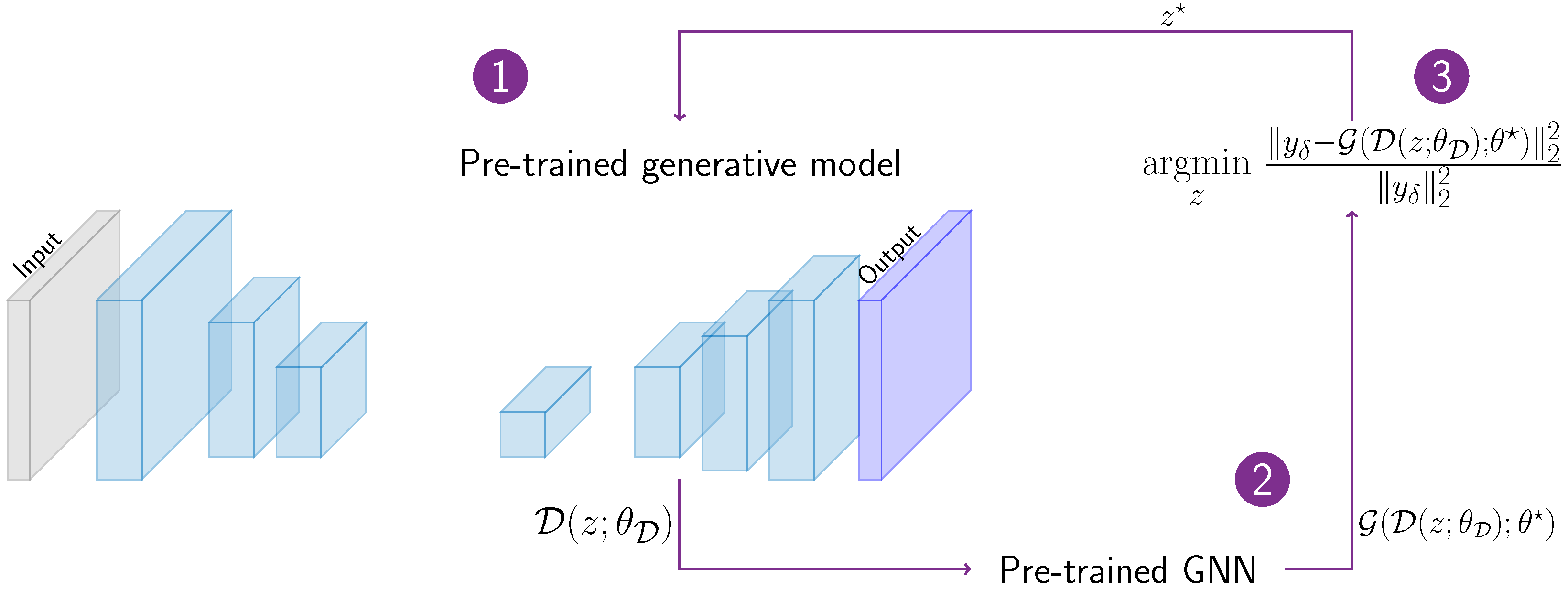
2.3. Learnable Prior

Since the image reconstruction in DOT is severely ill-posed due to the limited availability of boundary measurements and diffusive nature of near-infrared light propagation, we propose to regularize the problem by learning a prior to represent the solution space. To model the prior, we use the decoder part of a trained custom autoencoder, that is, a generative model mapping a low-dimensional latent space z to guess for the optical absorption coefficient ${\mu }_a$. To do this, we first consider a deterministic autoencoder architecture, composed of two subnetworks, an encoder $\mathcal{E}:{\mathbb{R}}^n\to {\mathbb{R}}^k$ and a decoder $\mathcal{D}:{\mathbb{R}}^k\to {\mathbb{R}}^n$, and we modify its structure by adding between the encoder and the decoder an additional linear layer $M:=M_t(M_{t-1}\dots \left(M_1\left(x\right)\right))\in {\mathbb{R}}^{k\times k}$, where $M_j\in {\mathbb{R}}^{k\times k},j=1,\dots ,t$ are randomly initialized trainable linear matrices, which provide better interpolation capabilities by minimizing the rank of the covariance matrix of the latent space [31]. In this way, we enforce many singular values to be equal to zero, removing the noise effect over the decoder, which leads to improved reconstructions. The resulting network is then trained to minimize the loss:

$$({\theta }_{\mathcal{D}}^{\ast },{\theta }_{\mathcal{E}}^{\ast })=arg\underset{{\theta }_{\mathcal{D}},{\theta }_{\mathcal{E}}}{min}\sum _i\parallel {\mu }_a^i-\mathcal{D}(M(\mathcal{E}({\mu }_a^i;{\theta }_{\mathcal{E}});{\theta }_M),{\mu }_a^i;{\theta }_{\mathcal{D}})){\parallel }_2^2.$$

(13)

Once trained, this autoencoder shows a low-rank latent space with sharply decreasing singular values and benefits from the large data dimensionality of the latent space to find better approximations while enhancing the model generative capabilities due to the low rank constraint on the latent space [32,33,34].

2.4. Learning the Inverse Problem Solution

Combining the learned Graph Neural Network and the autoencoder-type prior [23,24], we perform DOT reconstruction via the optimization procedure:

$$z^{\ast }=\underset{z}{argmin}{\displaystyle \frac{{\parallel y_{\delta }-\mathcal{G}(\mathcal{D}(z;{\theta }_{\mathcal{D}});{\theta }^{\ast })\parallel }_2^2}{{\parallel y_{\delta }\parallel }_2^2}},$$

(14)

where the pretrained GNN modeling the forward solver and the pretrained autoencoder as the prior are both fixed, and the latent code $z\in {\mathbb{R}}^k$ is optimized for a given set of sparse observations $y_{\delta }$, using an iterative procedure. The overall strategy is depicted in Figure 1.

3. Results

In this section, we present the numerical results on several test cases. All the computations have been run on the HPC cluster INDACO owned by University of Milan, equipped with Nvidia H100 GPUs (3.25 GHz, 32 cores, 384 GB RAM).

3.1. Generation of Synthetic Data

In our experiments, we consider the COULE (Contrasted Overlapping Uniform Lines and Ellipses) dataset [35], a collection of images designed to train and test neural networks for CT applications in medical imaging. The original COULE dataset consists of $256\times 256$ grayscale images of contrasted ellipses that resemble human anatomy. In this work, we have downsized the images to $32\times 32$ and we have considered in each image only a limited number of ellipses which, in our context, represent areas of augmented optical absorption coefficient (the Matlab R2024b code used to produce the simplified COULE dataset along with 10,000 generated samples are available at the link https://github.com/AleBenfe/GenDOT, last access 5 May 2025). We have also included purely circular regions. These simplifications are adherent to the literature of DOT reconstruction, which is notoriously a much more ill-conditioned problem than CT. The contrast regions are allowed to overlap and their size, absorption intensity, and position vary randomly. The background absorption coefficient, the diffusion coefficient, and the reduced scattering coefficient are, respectively, set to ${\mu }_{a,0}=0.01$ ${\mathrm{cm}}^{-1}$, $D=0.01$ cm, and ${\mu }_s^{\prime }=50$ ${\mathrm{cm}}^{-1}$. In the numerical experiments, light sources are uniformly located on the left, top, and right parts of the domain and the detectors are positioned on the whole boundary of the domain (configuration A) or, alternatively, light sources are uniformly located on the bottom part of the domain and the detectors are located on the other three sides (configuration B). For both configurations, the number of light sources is specified in each numerical example, while the number of detectors always corresponds to the resolution on each side. We refer to Figure 2, left and right panels, for a visualization.

We generated a set of 51,000 samples, each including one elliptic with random axes chosen in [0.1, 0.2] and two circular contrast regions with random radius chosen in [0.1, 0.2]: the position of these contrast regions are randomly selected inside the domain ${[0,1]}^2$. The contrast regions were chosen to have random absorption coefficient in the range (0.01, 0.07) cm⁻¹. This is consistent with the visual intensity scales used in Figure 3a, Figure 4a, Figure 5, and Figure 6 derived from the numerical experiments below. For each coefficient, the corresponding light fluence measurements at the detectors locations are generated by accurately solving the Diffusion Approximation model (3) via the quadratic Finite Element method implemented in the MatLab R2024b PDE Toolbox (version 24.2). We used 50,000 coefficient samples for training and 1000 for testing the autoencoder-type prior. The same sets of training and test data, each paired with their corresponding solutions, were also used to train and evaluate the Graph Neural Network.

3.2. Neural Architectures

The proposed DOT reconstruction framework combines two different kinds of neural network: a Graph Neural Network that serves as a forward model and a deterministic Autoencoder as a prior for the inverse problem solution.

3.2.1. Graph Neural Network Design

In (10), we set the width n of the Graph Neural Network to be 64, the number of iterations T to be 6, $\sigma$ to be the ReLU activation function, and we initialize $W\in {\mathbb{R}}^{64\times 64}$ as a random tensor drawn from a uniform distribution. The inner kernel network ${\kappa }_{\varphi }:{\mathbb{R}}^6\to {\mathbb{R}}^{4096}$ takes in input the edge features $e(x,y)=(x,y,{\mu }_a\left(x\right),{\mu }_a\left(y\right))$ and outputs a $64\times 64$ tensor and it is parameterized as a 3-layer feed-forward network with widths $(6;1024;1024;n^2)$ and ReLU activation function. The domain of integration $\mathsf{\Omega }$ is restricted to the ball $B_r\left(x\right)$ with radius $r=0.1$, which means that each node x is only connected to the nodes y that lie within the ball. In (9) and (11), we parametrize $\mathcal{P}$ and $\mathcal{Q}$ as 1-layer feed-forward networks with widths $(nodefeatures,width)=(3,64)$ and $(width,out\_width)=(64,1)$, respectively. We train the network for 200 epochs with respect to the absolute mean squared error on the normalized data, using the Adam optimizer with learning rate ${10}^{-4}$. We employ the message passing network from the standard graph network library PyTorch Geometric 2.7.0 [36].

Figure 3 shows the solution produced by the GNN for a test sample of absorption coefficient ${\mu }_a$. The model is trained on the dataset with resolution $32\times 32$ and tested on the same resolution. The light fluence approximation obtained with the GNN closely matches the ground truth solution.

To illustrate the GNN generalization capability across different grid resolutions [37], the model is trained on samples from a $32\times 32$ grid and tested on samples from a finer grid with resolution $64\times 64$. As shown in Figure 4, the GNN predicts similarly accurate solutions when tested on the finer grid, indicating that the learned GNN parameters are optimal when used with different resolutions.

3.2.2. Autoencoder Design

To model the prior, we used a deterministic autoencoder, with an encoder–decoder structure. The dataset of coefficients is normalized in the range [0, 1] and is given as input to the encoder which consists of convolutional layers with ReLU activation functions, followed by a sequence of linear layers of width equal to the latent space. The number t of linear layers is a hyperparameter and needs to be optimized in practice. Experiments showed that the best architecture has depth $t=4$. The generated latent space has size $k=32$. Notice that, by analyzing the singular values of the latent data covariances of the autoencoder applied to the present dataset, we estimate an intrinsic manifold dimension $d=16$. While the intrinsic dimension was estimated as 16, using 32 latent variables led to better empirical performance.

The decoder part consists of transposed convolutional layers, with ReLU activation functions applied to the first four layers and a Tanh activation function used in the final layer. We train the network with Adam optimizer for 100 epochs using a batch size of 1 and a learning rate of ${10}^{-4}$, in order to minimize the mean squared error loss between the ground truth coefficient and the coefficient generated by the composition of the encoder, the sequence of linear layers and the decoder. At inference time, the sequence of linear layers is treated as a single linear layer by simply computing the product of the sequence and it is incorporated into the last layer of the encoder, resulting in no change to the overall capacity of the autoencoder. The structure of the proposed autoencoder, which is employed during both training and inference phases, is described in detail in

Table 1. Structure of the autoencoder. The first 9 layers, as well as the liner layers, compose the encoder. The remaining layers define the decoder.

Layer Type	Output Shape	Kernel Size	Stride	Padding
Conv2d	[−1, 32, 16, 16]	(4, 4)	(2, 2)	(1, 1)
ReLU	[−1, 32, 16, 16]	-	-	-
Conv2d	[−1, 64, 8, 8]	(4, 4)	(2, 2)	(1, 1)
ReLU	[−1, 64, 8, 8]	-	-	-
Conv2d	[−1, 128, 4, 4]	(4, 4)	(2, 2)	(1, 1)
ReLU	[−1, 128, 4, 4]	-	-	-
Conv2d	[−1, 256, 2, 2]	(4, 4)	(2, 2)	(1, 1)
ReLU	[−1, 256, 2, 2]	-	-	-
Conv2d	[−1, 32, 1, 1]	(2, 2)	(1, 1)	(0, 0)
Linear	[−1, 32]	-	-	-
Linear	[−1, 32]	-	-	-
Linear	[−1, 32]	-	-	-
Linear	[−1, 32]	-	-	-
ConvTranspose2d	[−1, 256, 2, 2]	(2, 2)	(1, 1)	(0, 0)
ReLU	[−1, 256, 2, 2]	-	-	-
ConvTranspose2d	[−1, 128, 4, 4]	(4, 4)	(2, 2)	(1, 1)
ReLU	[−1, 128, 4, 4]	-	-	-
ConvTranspose2d	[−1, 64, 8, 8]	(4, 4)	(2, 2)	(1, 1)
ReLU	[−1, 64, 8, 8]	-	-	-
ConvTranspose2d	[−1, 32, 16, 16]	(4, 4)	(2, 2)	(1, 1)
ReLU	[−1, 32, 16, 16]	-	-	-
ConvTranspose2d	[−1, 1, 32, 32]	(4, 4)	(2, 2)	(1, 1)
Tanh	[−1, 1, 32, 32]	-	-	-

.

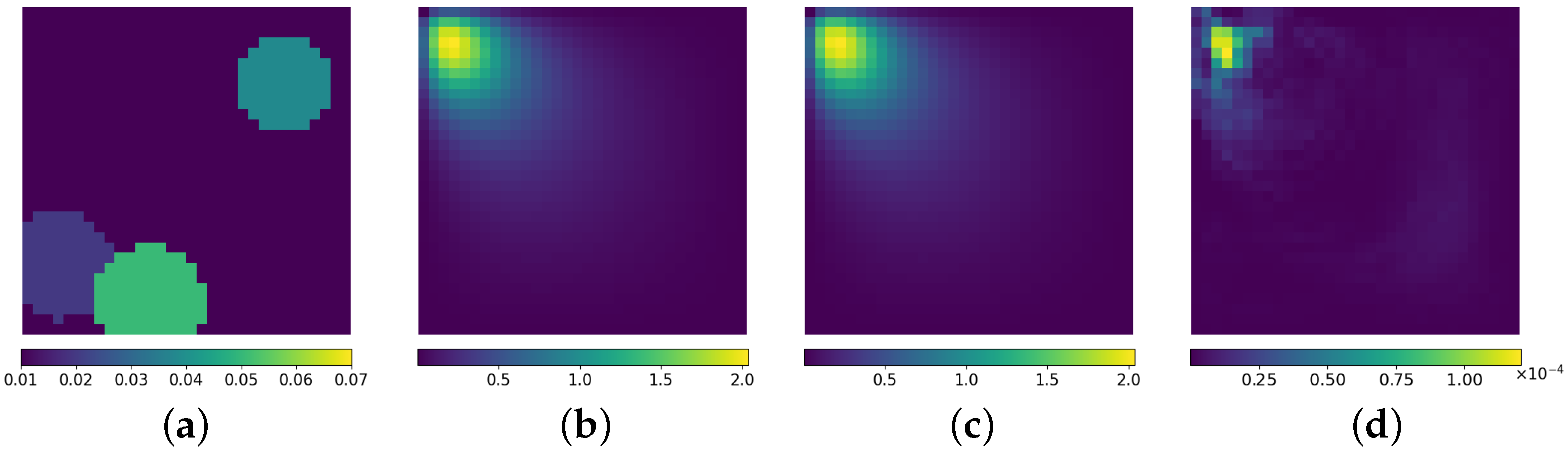
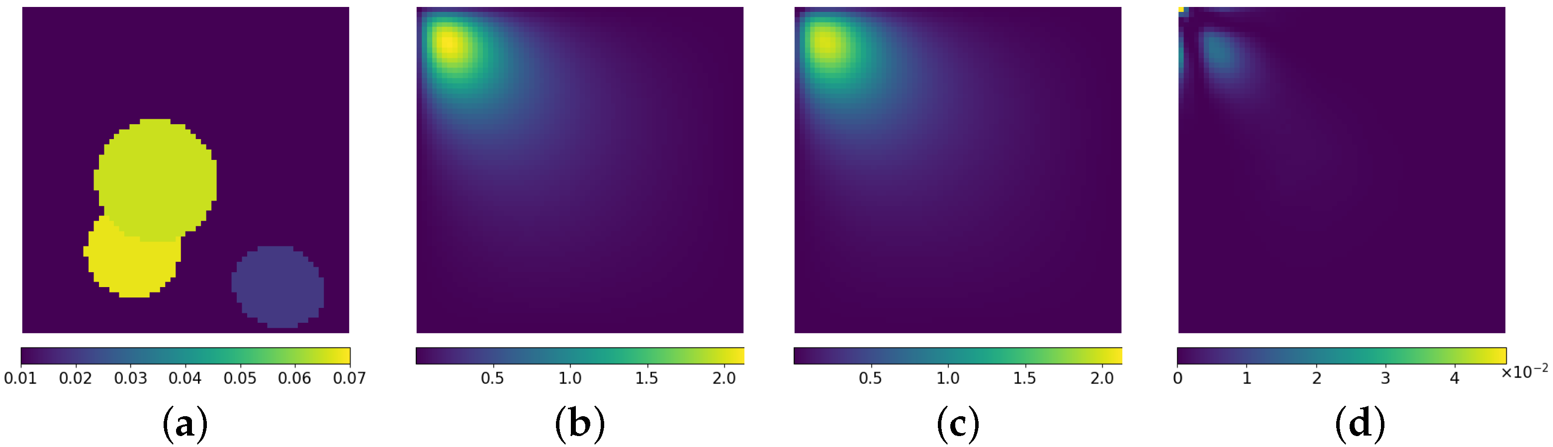
3.3. Inverse Problem

We solve the optimization Problem (14) with respect to the latent code z using the Adam optimizer with a learning rate of ${10}^{-4}$ for 1200 steps. To improve the generalization capabilities of the learned decoder, during the optimization we also perform a fine-tuning procedure of the prior after 200 steps, by optimizing the parameters of the decoder ${\theta }_{\mathcal{D}}$ using the Adam optimizer with a learning rate of ${10}^{-6}$. Larger values of the learning rate have been observed to determine strong cartoon effects in the image reconstruction. Figure 5 presents the results obtained for five different samples in the test set (Figure 5a) with 1 and 20 light sources (Figure 5b,c, respectively). During the inverse problem optimization loop, we consider in the loss function contributions of the observations corresponding to each light source. In the case of a single light source, this is located in the top-left corner of the domain, whereas in the cases of multiple sources these are uniformly distributed in the top, left, and right parts of the image, respectively. To provide a quantitative evaluation of the performance of the method, we compute the structural similarity index measure (SSIM) and the mean absolute error (MAE), averaged over 50 test (never seen) samples. The results are reported in

Table 2. Quantitative metrics on test image reconstruction.

	SSIM	MAE
Reconstruction using 1 light source	0.305	0.023
Reconstruction using 20 light sources	0.375	0.008

. SSIM and MAE values improve using more light sources and the reconstruction quality is improved in correspondence of areas with high-intensity absorption coefficient. One should notice that these values are not comparable with those one could obtain with standard X-ray tomography, which are way better, but in this context are to be considered as a remarkable result.

To assess the effectiveness of the proposed learned prior, we solve the DOT inverse problem without the pre-trained autoencoder (Figure 6b) and we also use classic variational methods with Bregman (Figure 6c) and Elastic Net regularization (Figure 6d). The two latter methods are implemented as described in detail in [12]. It is apparent that the severe ill-posedness of the reconstruction problem makes the solution hard to achieve due to coarse discretization, as already observed in [21].

4. Discussion

DOT reconstruction is a severely ill-conditioned problem and it requires a robust regularization. Papers from 1990s throughout the first decade of the 2000s typically use ${\ell }_2$ and/or ${\ell }_1$ or TV regularizations added to the discrepancy functional. Despite this, reconstruction results are often very poor even in settings so simple that they are extremely far from being realistic. The idea underlying the present work is that regularizing corresponds to assuming a prior on the solution (for example, a Gaussian prior in the case of the ${\ell }_2$ regularization) and modern generative models can be exploited to produce data-driven priors. The numerical results presented above show that this proposed framework has the potential to enhance the quality of the reconstruction when compared to conventional approaches. Specifically, as the number of available observations increases, our framework—combining a forward solver with a learnable prior—provides improved ability to estimate the general location and shape of contrast regions. It remains true, however, that the reconstruction becomes more challenging when the contrast regions overlap or are situated near the boundary of the domain: in these cases, the method is not able to capture the fine details of edges of overlapping contrast regions, resulting in a certain degree of blurring of the solution. As a side note, in the context of the forward problem, the most notable advantage of using a Graph Neural Network is that the learned network parameters are resolution independent, enabling consistent accuracy across inputs of different resolutions without requiring further adjustment of the net. This offers a significant improvement over classical neural network-based approaches for repeatedly solving PDEs.

5. Conclusions

In this work, we have addressed the solution of the ill-posed inverse problem arising from DOT reconstruction. This is a notoriously severely ill-conditioned problem which requires a robust regularization. In our approach, we have proposed to use a generative model, formed by the decoder part of a standard autoencoder, to serve as a prior generator for the unknown optical field. The generated prior is expected to lie near the training data manifold. The produced guess is then given as an input to a learned Graph Neural Network solver, which produces a solution to be compared with measured data, driving optimization iterations. The proposed framework has been evaluated on multiple test cases, and the experimental results suggest that incorporating the learned prior leads to improved reconstruction accuracy, especially when compared to standard approaches. As a last remark, one should note that when considering the results, the DOT technology is much more delicate than CT: the DOT signal to be reconstructed is indeed comparable to an extremely low-dose CT, a topic at the frontier of the present research. In conclusion, this work lays the groundwork for a new class of hybrid methods in inverse problem-solving for DOT. The promising results advocate for extending exploration at the intersection of deep generative modeling and learned physics-based solvers, potentially enabling more accurate and practical imaging tools for biomedical diagnostics.

References

1. Hoshi, Y.; Yamada, Y. Overview of diffuse optical tomography and its clinical applications. J. Biomed. Opt. 2016, 21, 091312. [Google Scholar] [CrossRef] [PubMed]
2. Jiang, H. Diffuse Optical Tomography: Principles and Applications; CRC Press: Boca Raton, FL, USA, 2018. [Google Scholar]
3. Wang, L.; Wu, H.I. Biomedical Optics: Principles and Imaging; John Wiley & Sons: Hoboken, NJ, USA, 2012. [Google Scholar]
4. Azar, F.S.; Lee, K.; Khamene, A.; Choe, R.; Corlu, A.; Konecky, S.D.; Sauer, F.; Yodh, A.G. Standardized platform for coregistration of nonconcurrent diffuse optical and magnetic resonance breast images obtained in different geometries. J. Biomed. Opt. 2007, 12, 051902. [Google Scholar] [CrossRef] [PubMed]
5. Arridge, S.; Maass, P.; Öktem, O.; Schönlieb, C.B. Solving inverse problems using data-driven models. Acta Numer. 2019, 28, 1–174. [Google Scholar] [CrossRef]
6. Benning, M.; Burger, M. Modern regularization methods for inverse problems. Acta Numer. 2018, 27, 1–111. [Google Scholar] [CrossRef]
7. Arridge, S.R.; Schotland, J.C. Optical tomography: Forward and inverse problems. Inverse Probl. 2009, 25, 123010. [Google Scholar] [CrossRef]
8. Lee, O.; Kim, J.M.; Bresler, Y.; Ye, J.C. Compressive diffuse optical tomography: Noniterative exact reconstruction using joint sparsity. IEEE Trans. Med. Imaging 2011, 30, 1129–1142. [Google Scholar] [CrossRef] [PubMed]
9. Egger, H.; Schlottbom, M. Analysis and regularization of problems in diffuse optical tomography. SIAM J. Math. Anal. 2010, 42, 1934–1948. [Google Scholar] [CrossRef]
10. Kazanci, H.O.; Jacques, S.L. Diffuse Light Tomography to Detect Blood Vessels Using Tikhonov Regularization. Proc. SPIE 2016, 9917, 99170S. [Google Scholar] [CrossRef]
11. Aspri, A.; Benfenati, A.; Causin, P.; Cavaterra, C.; Naldi, G. Mathematical and numerical challenges in diffuse optical tomography inverse problems. Discret. Contin. Dyn. Syst. S 2023, 17, 421–461. [Google Scholar] [CrossRef]
12. Benfenati, A.; Lupieri, M.; Naldi, G.; Causin, P. Regularization Techniques for Inverse Problem in DOT Applications. J. Phys. Conf. Ser. 2020, 1476, 012007. [Google Scholar] [CrossRef]
13. McCann, M.T.; Jin, K.H.; Unser, M. Convolutional Neural Networks for Inverse Problems in Imaging: A Review. In IEEE Signal Process. Mag. 2017, 34, 85–95. [Google Scholar] [CrossRef]
14. Zheng, B.; Andrei, S.; Sarker, M.K.; Gupta, K.D. Data Driven Approaches on Medical Imaging; Springer: Cham, Switzerland, 2024. [Google Scholar] [CrossRef]
15. Patra, R.; Dutta, P.K. Improved DOT reconstruction by estimating the inclusion location using artificial neural network. Med. Imaging 2013 Phys. Med. Imaging 2013, 8668, 86684C. [Google Scholar] [CrossRef]
16. Sun, Y.; Xia, Z.; Kamilov, U.S. Efficient and accurate inversion of multiple scattering with deep learning. Opt. Express 2018, 26, 14678–14688. [Google Scholar] [CrossRef] [PubMed]
17. Feng, J.; Sun, Q.; Li, Z.; Sun, Z.; Jia, K. Back-propagation neural network-based reconstruction algorithm for diffuse optical tomography. J. Biomed. Opt. 2018, 24, 1–12. [Google Scholar] [CrossRef] [PubMed]
18. Yoo, J.; Sabir, S.; Heo, D.; Kim, K.H.; Wahab, A.; Choi, Y.; Lee, S.-I.; Chae, E.Y.; Kim, H.H.; Bae, Y.M.; et al. Deep Learning Diffuse Optical Tomography. IEEE Trans. Med. Imaging 2020, 39, 877–887. [Google Scholar] [CrossRef] [PubMed]
19. Deng, B.; Gu, H.; Carp, S.A. Deep learning enabled high-speed image reconstruction for breast diffuse optical tomography. Opt. Tomogr. Spectrosc. Tissue XIV 2021, 11639, 116390B. [Google Scholar] [CrossRef]
20. Mozumder, M.; Hauptmann, A.; Nissila, I.; Arridge, S.R.; Tarvainen, T. A Model-Based Iterative Learning Approach for Diffuse Optical Tomography. IEEE Trans. Med. Imaging 2022, 41, 1289–1299. [Google Scholar] [CrossRef] [PubMed]
21. Benfenati, A.; Causin, P.; Quinteri, M. A Modular Deep Learning-based Approach for Diffuse Optical Tomography Reconstruction. arXiv 2024, arXiv:2402.09277. [Google Scholar]
22. Herzberg, W.; Rowe, D.B.; Hauptmann, A.; Hamilton, S.J. Graph Convolutional Networks for Model-Based Learning in Nonlinear Inverse Problems. IEEE Trans. Comput. Imaging 2021, 7, 1341–1353. [Google Scholar] [CrossRef] [PubMed]
23. Zhao, Q.; Lindell, D.B.; Wetzstein, G. Learning to Solve PDE-Constrained Inverse Problems with Graph Networks. In ICML; 2022; Available online: https://icml.cc/media/icml-2022/Slides/16566.pdf (accessed on 22 July 2025).
24. Zhao, Q.; Ma, Y.; Boufounos, P.; Nabi, S.; Mansour, H. Deep Born Operator Learning for Reflection Tomographic Imaging. In Proceedings of the ICASSP 2023—2023 IEEE International Conference on Acoustics, Speech and Signal Processing (ICASSP), Rhodes Island, Greece, 4–10 June 2023; pp. 1–5. [Google Scholar] [CrossRef]
25. Durduran, T.; Choe, R.; Baker, W.B.; Yodh, A.G. Diffuse Optics for Tissue Monitoring and Tomography. Rep. Prog. Phys. 2010, 73, 076701. [Google Scholar] [CrossRef] [PubMed] [PubMed Central]
26. Haskell, R.C.; Svaasand, L.O.; Tsay, T.T.; Feng, T.C.; McAdams, M.S.; Tromberg, B.J. Boundary conditions for the diffusion equation in radiative transfer. J. Opt. Soc. Am. A 1994, 11, 2727–2741. [Google Scholar] [CrossRef] [PubMed]
27. Evans, L.C. Partial Differential Equations; American Mathematical Society: Providence, RI, USA, 1998. [Google Scholar]
28. Roach, G.F. Green’s Functions, 2nd ed.; Cambridge University Press: Cambridge, UK, 1982. [Google Scholar]
29. Li, Z.; Kovachki, N.B.; Azizzadenesheli, K.; Liu, B.; Bhattacharya, K.; Stuart, A.M.; Anandkumar, A. Neural Operator: Graph Kernel Network for Partial Differential Equations. arXiv 2020, arXiv:2003.03485. [Google Scholar]
30. Gilmer, J.; Schoenholz, S.S.; Riley, P.F.; Vinyals, O.; Dahl, G.E. Neural message passing for Quantum chemistry. In Proceedings of the 34th International Conference on Machine Learning (ICML’17), Sydney, Australia, 6–11 August 2017; Volume 70, pp. 1263–1272. [Google Scholar]
31. Arora, S.; Cohen, N.; Hu, W.; Luo, Y. Implicit regularization in deep matrix factorization. In Proceedings of the 33rd International Conference on Neural Information Processing Systems, Vancouver, BC, Canada, 8–14 December 2019; Curran Associates Inc.: Red Hook, NY, USA, 2019. Article 666. pp. 7413–7424. [Google Scholar]
32. Mazumder, A.; Baruah, T.; Kumar, B.; Sharma, R.; Pattanaik, V.; Rathore, P. Learning Low-Rank Latent Spaces with Simple Deterministic Autoencoder: Theoretical and Empirical Insights. In Proceedings of the IEEE/CVF Winter Conference on Applications of Computer Vision, Waikoloa, HI, USA, 3 January 2024; pp. 2851–2860. [Google Scholar]
33. Jing, L.; Zbontar, J.; LeCun, Y. Implicit rank-minimizing autoencoder. In Proceedings of the 34th International Conference on Neural Information Processing Systems, Vancouver, BC, Canada, 1 October 2020. [Google Scholar]
34. Mounayer, J.; Rodriguez, S.; Ghnatios, C.; Farhat, C.; Chinesta, F. Rank Reduction Autoencoders—Enhancing interpolation on nonlinear manifolds. arXiv 2024, arXiv:2405.13980. [Google Scholar] [CrossRef]
35. COULE Dataset. Available online: www.kaggle.com/loiboresearchgroup/coule-dataset (accessed on 15 April 2025).
36. PyG Documentation. Available online: https://pytorch-geometric.readthedocs.io/ (accessed on 5 May 2025).
37. You, H.; Yu, Y.; D’Elia, M.; Gao, T.; Silling, S. Nonlocal kernel network (NKN): A stable and resolution-independent deep neural network. J. Comput. Phys. 2022, 469, 111536. [Google Scholar] [CrossRef]
Figure 1. Proposed framework for DOT reconstruction. (1) The decoder part of the learned autoencoder maps the latent code to the estimated absorption coefficients. (2) The GNN solver takes as input the prior output and computes the measured light fluence. (3) The latent code is optimized to minimize the discrepancy between the ground truth light fluence and the measured light fluence.
Photonics 12 00746 g001
Figure 2. Location of light sources (yellow dots) and detectors (gray triangles) in the numerical experiments. (Left) panel, configuration A: the sources are uniformly located on the left, top, and right sides of the domain, while the detectors surround the whole domain. (Right) panel, configuration B: a different possible configuration, where the sources are located only on the bottom of the domain and the detectors are located on the other three sides (left, top, and right side).
Photonics 12 00746 g002
Figure 3. GNN performance on a test sample with resolution 32 × 32 . (a) Ground truth absorption coefficient. (b) Ground truth light fluence. (c) GNN approximation of the light fluence. (d) Absolute mean squared error between the ground truth in (b) and the approximation in (c).
Photonics 12 00746 g003
Figure 4. GNN performance on a test sample with resolution 64 × 64 obtained from a GNN trained on 32 × 32 samples. (a) Ground truth absorption coefficient. (b) Ground truth light fluence. (c) GNN approximation of the light fluence. (d) Absolute mean squared error between the ground truth in (b) and the approximation in (c).
Photonics 12 00746 g004
Figure 5. Reconstruction of the absorption coefficient distribution: (a) Ground truth. (b) Reconstruction using a single light source. (c) Reconstruction using 20 light sources. Each column corresponds to a different ground truth. For all images, the same colorbar is used, in the range (0.01, 0.07).
Photonics 12 00746 g005
Figure 6. Visualization of the reconstruction performance without the use of the prior computed via the generative approach. (a) Ground truth coefficient. (b) Reconstruction of the absorption coefficient distribution using the GNN solver without regularization. Reconstruction of the absorption coefficient distribution obtained from classic variational approaches using Bregman iterations (c) and Elastic Net regularization (d).
Photonics 12 00746 g006