Mie Coefficients

Department of Physics and Astronomy, Mississippi State University, P.O. Box 5167, Starkville, MS 39762-5167, USA
Photonics 2025, 12(7), 731; https://doi.org/10.3390/photonics12070731
Submission received: 27 May 2025
/
Revised: 9 July 2025
/
Accepted: 9 July 2025
/
Published: 18 July 2025
Abstract
We consider the scattering of electromagnetic radiation by a spherical particle, known as Mie scattering. The electric and magnetic fields are represented by multipole fields, and the amplitudes are the Mie scattering coefficients. Properties of the particle are mainly contained in these coefficients. We have studied the dependence of these coefficients on the various parameters, with an emphasis on the dependence on the particle radius. Central to this discussion is what is known as the ‘Mie circle’. Without absorption in the particle or the embedding medium, the Mie scattering coefficients lie on this universal circle in the complex plane. We have studied the location of the Mie scattering coefficients on this circle as a function of the particle radius. The Mie circle also serves as a reference for the case when there is absorption in the particle or the medium. In the limit of a small particle, a peculiar divergence appears in the expression for the Mie coefficients, known as the Fröhlich resonance. We show that this apparent singularity is a consequence of the fact that the limit of a small particle fails in the neighborhood of this resonance, and we derive an expression for the correct small-particle limit in the neighborhood of this resonance.
1. Introduction
The problem of the scattering of a plane wave by a spherical particle was solved more than a century ago by Gustav Mie [1]. This milestone achievement has found numerous applications, ranging from the detection of aerosols in the atmosphere to measurements of the radii of nano-sized particles. More recently, small dielectric Mie particles were considered for the building blocks of metamaterials [2,3,4]. An interesting phenomenon is the appearance of photonic jets in Mie scattering [5,6]. Numerous papers have been devoted to the numerical evaluation of the Mie coefficients [7,8,9,10,11,12,13,14,15,16,17], and comprehensive reviews of Mie scattering can be found in [18,19,20].
Figure 1 schematically shows the setup for Mie scattering. A particle with the radius R is located at the origin of coordinates. It has (relative) permittivity and (relative) permeability and the particle is embedded in a medium with permittivity and permeability A laser beam with angular frequency propagating into the positive direction, irradiates the particle. The wave number in free space is We set for the dimensionless radius of the particle, and we shall simply refer to this as the radius of the particle. On this scale, a distance of corresponds to an optical wavelength in free space. The incident radiation scatters off the particle, and part of it enters the particle. Mie theory provides the expressions for the electric and magnetic fields, both inside and outside of the particle, and for any values of the parameters.
The parameters and are complex, in general, and they depend on the angular frequency which is a constant in this problem. For causality reasons, these parameters lie in the upper half of the complex plane, or on the real axis [21] (p. 310), e.g.,
The index of refraction is the solution of This equation has two solutions, and we need the solution for which
A moment of thought then shows that the correct solution is
both for the embedding medium and the particle. For the square root function, we take the cut in the complex plane just below the negative real axis. It will turn out to be advantageous to introduce the particle parameters relative to the parameters of the embedding medium. We set
2. Incident Field
The incident field is a monochromatic polarized plane wave, with and as the complex amplitudes of the electric and magnetic fields, respectively. The electric field itself is
and similarly for the magnetic field. For the electric field, we have
Here, is the unit polarization vector, normalized as . This generally complex vector lies in the plane. The wave vector is with as the wave number in the embedding medium. The corresponding magnetic field is
We set
so that
This notation is particularly useful when studying electric and magnetic dipole radiation, as in Appendix C.
The index of refraction will be complex, in general. We set
With the time-dependent electric field from Equation (5) becomes
Due to the overall exponential, the field decays in amplitude into the positive direction if . The exponential factor inside is a traveling plane wave with phase velocity
For , the wave pattern moves into the positive direction, and for , it moves into the negative direction. It can be shown that the energy always flows into the positive direction.
In order to eliminate non-essential constants, we introduce dimensionless fields as
For the magnetic field, we take as for a field outside the particle and as for a field inside the particle. For the incident fields, this becomes
For Mie scattering, it is advantageous to consider circularly polarized incident radiation. We take as a spherical unit vector:
For , this gives a left-polarized plane wave, or a wave with positive helicity. The electric and magnetic field vectors rotate counterclockwise when viewed down the positive axis, with the magnetic field lagging the electric field by For the magnetic field, we have
so, the dimensionless incident fields are related as
For other polarizations of the incident field, the solution can be obtained by superposition.
3. Fields and Mie Coefficients
Mie theory provides the exact solution of Maxwell’s equations for the setup depicted in Figure 1. Since Mie’s paper, mathematics has evolved substantially, and the theory has been put on a more solid, and elegant, footing. Now, the fields are expanded onto a complete set of vector functions on the unit sphere, the vector spherical harmonics [22,23]. Each vector spherical harmonic is multiplied by a spherical Bessel function, and this gives a partial wave of the solution. This gives a consistent expansion of the fields in vector multipole fields.
The scattered fields are and and the particle fields are and Their explicit expressions in terms of multipole fields are given in Appendix A. We have electric (e) and magnetic (m) multipole fields, and the order of a multipole is indicated by The amplitudes of the scattered multipole fields are with and the amplitudes of the particle multipole fields are These are the Mie coefficients. It is outlined in Appendix B how these amplitudes are computed from the boundary conditions at the surface of the sphere. In most references, these Mie coefficients are expressed in terms of Riccati–Bessel functions and their derivatives. Although such representations are very compact, they are not very suitable for analysis. Appendix B gives various representations of the Mie coefficients. The Mie scattering coefficients take the form
and for the Mie particle coefficients, we have
Here,
Equations (A34) and (A35) give the most useful representations for the auxiliary functions and They only involve the spherical Bessel functions and the spherical Neumann functions The function can then be found from Equation (23). Alternatively, Equation (A36) can be used for which involves the spherical Hankel functions These are the functions for electric multipoles. They contain the parameter As explained in Appendix B, the corresponding magnetic multipole functions simply follow by replacing by This implies that any computation performed (as below) for electric multipoles automatically carries over to magnetic multipoles. Oddly enough, this is never recognized in the literature, to the best of our knowledge. The reason is probably that most authors set . This is a very good approximation for most materials, but it destroys the symmetry between electric and magnetic Mie coefficients. As a result, two sets of equations are presented, one for electric multipoles and one for magnetic multipoles, and all calculations need to be performed twice. Our approach is clearly much more efficient, and elegant.
A Mie resonance is defined as a situation where . It follows from Equation (21) that is a sufficient condition.
The lowest-order multipoles have representing electric and magnetic dipole radiation. By far the most studied radiation is electric dipole radiation, both in classical electromagnetism and quantum optics. It is shown in Appendix C that these multipole fields are identical to the textbook expressions for such radiation, as well as how the dipole moments of the particle can be obtained from the Mie scattering coefficients. For dipoles, the Mie coefficients can be expressed in terms of elementary functions rather than spherical Bessel functions. The explicit results for the dipole Mie coefficients are given in Appendix D.
Of particular interest is the ever-popular perfect conductor. Such material is impenetrable for electromagnetic radiation, and this gives huge simplifications for all types of problems. A perfectly conducting particle is a metallic particle in the limit where the conductivity becomes very large. In Appendix E, we derive the expressions for the Mie coefficients for a perfectly conducting particle.
4. Dielectric Particle
Central to Mie scattering are the Mie coefficients. In this section, we shall restrict the material parameters to
The conditions and represent a typical dielectric particle. None of the parameters has an imaginary part, so there is no absorption, or damping, in the particle or in the embedding medium. Then, the indices of refraction and are positive. The spherical Bessel functions and are real for . With Equations (A34) and (A35), we then see that the functions and are real. Let us now consider a complex number that can be written as
It follows immediately that
This represents a circle in the complex plane with radius 1/2 and centered at 1/2. We call this the Mie circle, and this circle is shown in Figure 2.
- In the Mie scattering coefficients, given by Equation (21), the functions and are real, and therefore they are of the form given in Equation (25). Consequently,
From Equation (27), we easily derive
5. Metallic Particle
In this section, we consider the important case of a metallic particle, without dissipation in the particle or the embedding medium. We then have
The index of refraction of the medium is positive, and the index of refraction of the particle is positive imaginary. We set
The auxiliary functions and given by Equations (A34), (A35) and (A36), respectively, contain the spherical Bessel functions Since the argument is imaginary, it becomes advantageous to set
with a modified Bessel function. This function is real for the real argument. We define the functions and by
The functions and then become
For magnetic multipoles, we set
In terms of these new functions, the Mie scattering coefficients take the form
We see from Equations (36) and (37) that and are real, and therefore lies on the Mie circle. This reflects again that there is no dissipation in the system. The particle Mie coefficients become
The Mie scattering coefficients for a perfect conductor are given by Equations (A86) and (A87). Both for electric and magnetic multipoles, they have the form of in Equation (25), so if there is no absorption in the embedding medium, then the Mie scattering coefficients for a perfectly conducting particle lie on the Mie circle.
6. Small Particle
Mie theory is particularly important for scattering off small particles. Here, ‘small’ means small in comparison with the wavelength of the radiation. Since we have we consider The auxiliary functions and are determined by the spherical Bessel functions and which appear with arguments and For small , we have
For , we find from Equation (A34)
Here, we have introduced the abbreviation
Table 1 lists for some values. We see that is already very small for moderate values. For , we obtain from Equation (A35)
The parameter is defined as
which lies in the range .
The function is and is so in , we can neglect This yields the results for small
For , we have but is finite.
In these expressions, there is a problem when is close to Since , this can happen for a metallic particle. We will come back to this issue in Section 11. For magnetic multipoles, we make the replacement Then, becomes proportional to which presents another problem. For most materials, we have and . Then, and the first term in goes to zero. For this case, we need one more term in the expansion for small This is found to be
For the case of a perfect conductor, we find from Equations (A86) and (A87)
Here, we notice that
so, the electric and magnetic multipole Mie coefficients have the same order of magnitude [25].
7. Large Particle
We now consider the opposite case of a large particle, so a particle with a radius larger than an optical wavelength. We use the asymptotic formulas for spherical Bessel functions
Rather than considering here it is better to consider
When is on the Mie circle, then is on the unit circle, and vice versa. We obtain the following from Equations (A34) and (A35):
For the Mie particle coefficients, we find
For magnetic multipoles, we replace Figure 4 shows and the large- approximation for the parameters given in the caption. We see that, apart from some tiny wiggles, the approximation is excellent for not too small. With increasing the Mie coefficient rotates around the Mie circle, and this gives the oscillations in the figure. At the maxima, we have and since this represents a point on the Mie circle, we have . Therefore, at a maximum in the graph, and this represents a Mie resonance. The above expressions for large hold for any combination of parameters. Let us now consider a metallic particle, as in Section 5. The index of refraction of the particle is positive imaginary, and we set with . We then have for the sines and cosines in Equations (56) and (57)
since . Equation (56) simplifies to
The right-hand side lies on the unit circle, so lies approximately on the Mie circle. Since for a metallic particle, lies on the Mie circle for all this has to be so. Equation (57) becomes
Rather than circling around the origin, as in Figure 3, spirals into the origin for a metallic particle, due to the overall factor This is illustrated in Figure 5. For magnetic multipoles, we replace in Equations (60) and (61). For a perfect conductor, we find the simple result
8. Rotation Directions
When there is no dissipation in the medium or particle, then lies on the Mie circle. For , we have and with increasing , the particle moves around the Mie circle. We shall now consider this in more detail. In order to simplify the discussion somewhat, we shall assume
For positive, this corresponds to a dielectric particle, as in Section 4, and for negative, this is a metallic particle, as in Section 5.
For small, is given by Equation (47). We recall that from Equation (46) lies in the range . If is smaller than then is smaller than unity, and the overall factor is positive. This means that is negative imaginary, so the rotation around the Mie circle starts counterclockwise. For , we also have and again and so the rotation is initially counterclockwise. For the region in between, e.g., , we have so is positive imaginary, and the rotation is clockwise. For , we need to consider Equation (49). For is negative imaginary, and the rotation starts counterclockwise. For this becomes clockwise. This is made much clearer by looking at Figure 6.
For large , we need to consider Equation (56) for . Then, we also have . With the factor rotates around the unit circle in the clockwise direction with increasing The period for this rotation follows from The first factor in square brackets in Equation (56) is periodic with given by Due to the factors and this factor rotates over an ellipse, and it goes counterclockwise. The factor in square brackets in the denominator also gives a counterclockwise rotation with The two factors combined then give a counterclockwise rotation with The period for the rotation of around the unit circle then becomes We conclude that for , the rotation is counterclockwise, and for , the rotation is clockwise. Since we consider in this section, this is equivalent to and respectively, (and in this paragraph). For large and , we have a metallic particle, and the result for large is given by Equation (60). The only rotation is due to the factor and this rotates clockwise.
For with we have Equation (49) for small. The rotation direction only depends on so we have counterclockwise for and clockwise for . For large, there is no difference in the rotation direction between and given
The Mie particle coefficients for small are given by Equation (48), and with , we find the expression for These functions are finite for . For positive, we have positive, and so lies on the positive real axis. For negative, we have and so is proportional to Therefore, lies on the real or imaginary axis, either at the positive or negative side, and when we increase the value of by unity, the picture rotates clockwise over The Mie particle coefficients do not have a specific rotation direction for small.
For large, we consider Equation (57), when . With the same arguments as above for we now find that rotates clockwise for and counterclockwise for . However, the rotation is around the origin and not around the Mie circle, and the path is not circular. An example is shown in Figure 3. For we look at Equation (61). The only rotation comes from and this gives a clockwise rotation. For large , we have due to the factor An example is show in Figure 5. The three possibilities are illustrated in Figure 7.
For a perfect conductor, the rotation directions of are the same as those in Figure 6 for
9. Turning Points
The rotation directions of the Mie scattering coefficients around the Mie circle are depicted in Figure 6. We see that the initial rotation directions () and the final rotation directions () are the same, except for when In this case, the rotation starts counterclockwise and ends clockwise. Therefore, the curve has a turning point at which the rotation direction reverses. We shall now examine this in detail. Figure 8 shows an example. At a turning point, it has to hold that
The derivatives of the Mie scattering coefficients with respect to are derived in Appendix F. In this section, we shall assume and we have for a turning point to occur. Since is complex, Equation (65) has to hold for the real and imaginary parts of simultaneously. Figure 9 shows the real and imaginary parts of the derivative of for the same parameters as in Figure 8. We see that near both the real and imaginary parts of are zero, so this is the turning point
Near a turning point, is neither small nor large, so we need to consider the exact solution for all From Equation (A93), we see that for
the derivative of is zero. Under this condition, the real and imaginary parts are simultaneously zero. Here, we have with so the arguments of and are positive imaginary. Then, it is advantageous to switch to modified Bessel functions, as in Equation (32). Equation (66) becomes
Here, we have set
which is positive. Setting simplifies the appearance of Equation (67) to
Both sides of the equation are squares. With recursion relations for modified Bessel functions, it can be shown that
With the known series expansions of the modified Bessel functions, we find easily that and its derivative are positive for . Therefore, the right-hand side of Equation (70) is positive. Then, the expression in square brackets on the left-hand side of Equation (69) is positive, as is on the right-hand side. Consequently, we can take the square roots of both sides as
We now set
A turning point then corresponds to a solution of
For a solution the turning point is
Figure 10 shows the function seen as a function of for 1, 2 and 3, and for . The zeros are found from the graph as and respectively. Alternatively, Equation (73) can easily be solved numerically, which would give more precise values for
Equation (73) can be written as
and the parameter is
For very negative, this parameter becomes large. Then, is large, and we can consider the modified Bessel functions for the large argument:
The right-hand side is independent of , so Equation (75) becomes
and this is
For large, and with
the first on the right-hand side of Equation (79) can be neglected. At a turning point, we have so the turning point is approximately
for large. For the examples in Figure 10, this gives 0.71, 1.22 and 1.73 for and respectively. We have verified that the accuracy of this approximation improves considerably with increasing
For very large, the particle approaches the perfect conductor limit. The derivative of is given by Equation (A95). At a turning point, this should be zero, which gives
and this is
Clearly, the approximate value from Equation (81) becomes the exact solution for a perfect conductor.
10. Dissipation in the Particle
When there is no absorption in the particle or the embedding medium, the Mie scattering coefficients lie on the Mie circle, and they rotate around this circle with increasing We shall now consider the effect of damping in the particle. We set so that there is no absorption in the surrounding medium. For the particle material, we shall assume and possibly .
The coefficients are zero for . For small the value of is given by Equation (47), and with , this gives provided that . For we need to consider Equation (49). Without absorption, is pure imaginary, so with increasing the rotation starts either up or down the imaginary axis. This is expected, because the imaginary axis is the tangent line at the Mie circle at . With absorption, has a real part, and so the initial direction with increasing is under an angle with the imaginary axis. Equation (47) reads
For real, the shown factor is imaginary. For complex, we set Under the assumption that the damping is relatively small, we then find
with
which is positive. Therefore, and the curve in the complex plane bends away from the imaginary axis to the right. From a different point of view, moves to the inside of the Mie circle. The initial direction along the imaginary axis is the same as without absorption, provided we replace by its real part. For , we assume and it then follows immediately from Equation (49) that the same conclusion holds.
For large the general expression is given by Equation (56). We shall now simplify this result for the case that there is damping in the particle. The particle index of refraction is complex, and we write
For the sines and cosines in Equation (56), we use . This yields
Both terms grow exponentially with due to the factors Fortunately, these factors appear both in the numerator and denominator, so they cancel. We obtain
for large. For magnetic multipoles, we replace by and we use the identity
This gives
which differs from by only a minus sign.
The only rotation in comes from which is clockwise, and the path in the complex plane is a circle around the origin. Then, rotates clockwise around the point 1/2, and the radius of the circle is
This circle is concentric with the Mie circle, and we shall call this the reduced Mie circle. The radius is the same for electric and magnetic multipole coefficients. Also interesting to see is that the rotation direction for large is the same for all parameters. This is in contrast to the case without damping, where the rotation is counterclockwise for (Figure 6). We note that the reduced Mie circle does not necessarily go over in the Mie circle in the limit of no damping. We have used to arrive at Equations (88) and (89), and this excludes the limit .
Figure 11 summarizes the rotation directions for the case when there is damping in the particle. The initial rotation direction is determined by the real part of and the curves start under an angle with the imaginary axis such that the damping gives a deviation to the right. For , we assumed . The final directions for all cases are clockwise, so this is independent of As compared to Figure 6, we see that for the rotation direction is opposite to the case without damping, so the dissipation in the particle reverses the final rotation direction. Since this direction is opposite to the initial rotation direction, the Mie coefficients must have a turning point due to the absorption of energy in the particle.
Figure 12 shows a typical curve in the complex plane. The rotation direction is clockwise for all and for large, the curve approaches the reduced Mie circle. Another example is shown in Figure 13. The initial rotation is counterclockwise, but then the direction reverses and becomes clockwise by the time it reaches the reduced Mie circle. A similar case is shown in Figure 14, but now we can clearly see the predicted turning point. Without absorption, the rotation direction would be counterclockwise for all
The Mie particle coefficient at is given by Equation (48), and the value of at follows from They are finite, but they do not lie on an axis as they do without damping. With a similar calculation as above, we find for large
and for , we replace with For large due to the factor The Mie coefficients spiral into the origin, unlike without damping, where this only happens for (Figure 7). The rotation around the origin comes from The rotation is counterclockwise for and clockwise for A typical example is shown in Figure 15.
11. Dissipation in the Medium
Let us now consider the effect of damping in the embedding material. We shall assume so that there is no absorption in the particle, and we set , as in Equation (11). Here, is real, and is positive. The behavior of for large follows from Equation (56). We find
and for the Mie particle coefficients, we find from Equation (57)
For magnetic multipoles, we replace With the same reasoning as in Section 8, we see that the rotation direction is counterclockwise for and clockwise for The Mie coefficient rotates around the Mie circle, and rotates around the origin.
The most striking feature is the factors in and in These factors grow exponentially with the particle radius When there is damping in the particle, moves to the inside of the Mie circle and eventually starts to rotate around the reduced Mie circle, as illustrated in Figure 13 and Figure 14. The coefficients spiral into the origin with increasing as shown in Figure 15. Due to damping in the surrounding medium, the effect is the opposite. The coefficients spiral away from the Mie circle and continue to grow without bounds with increasing This is illustrated in Figure 16. Also, grows exponentially, as shown in Figure 17. When there is damping in the particle and in the host medium, it depends on which one ‘wins’. Figure 18 depicts this combined effect. Initially, the curve tends to go to the inside of the Mie circle as a result of the damping in the particle, but eventually it turns to the outside and keeps on growing.
12. The Fröhlich Mode
It was shown in Section 6, Equation (47), that for small we have
with We notice immediately that there is a problem if is close to and since is negative, this can happen easily for a metallic particle. This situation is referred to as the Fröhlich resonance, or the Fröhlich mode. The Mie particle coefficient from Equation (48) has the same problem. A division by zero would give an infinite Mie coefficient, which is unphysical. Moreover, we know that without damping, lies on the Mie circle. The magnetic multipole Mie coefficients do not have this issue (unless one would consider which is unrealistic), so in this section, we shall only consider electric multipoles. It is often argued in the literature that one should include a small positive imaginary part in in order to keep finite. We shall show below that this gives the wrong result [26]. This issue was also addressed in [27], from a different point of view.
The small- limit of the Mie coefficients was derived in Section 4, starting from the representations (21) and (22). We expanded the functions and in a Taylor series in with the results given by Equations (43) and (45). In the numerators, we have Since is of a much higher order in we neglected in and this gave the results shown in Equations (47) and (48). From Equation (45) we see that is zero at and this is the root of the problem with the approximation (97), and similarly for . When we need to retain in First, we change to alternative and
which are more suitable for the study of small. The Mie coefficients are then
with From here on, we shall use an equal sign instead of for the small- approximation. For , we keep the result from Equation (43):
but for , we add one more term in the Taylor expansion for small This gives
Here, we introduced the parameter
The new and improved small- approximations to the Mie coefficients are then given by Equations (100) and (101).
First, we notice that the singularities for near have disappeared. Second, without damping in the particle or the surrounding medium, and are real. So, has the same form as in Equation (25), and therefore the approximation lies on the Mie circle. This reflects conservation of energy, even for the approximate formula. Third, for we have and so this resonance is a Mie resonance in the true sense of the meaning. As a consistency check, consider a transparent particle. Then, and we immediately find , and so . From Equation (104), we see that and with , we find .
Figure 19 shows as a function of and the small- approximation. We have which is close to for . Figure 20 shows for the same parameters. We notice that the approximation is excellent. Another thing to see is that the exact curve indeed gives a resonance, where (and not shown in the graph). It can also be verified that for parameters not near the Fröhlich resonance, the new approximation for small is a huge improvement, as compared to Equation (97).
For the remainder of this section, we shall set μ1 = 1,
. Then, from Equation (104) simplifies to
with
With Equation (46) we have
Since we have and we also see that lies in the range . Table 2 shows various values of and
Function from Equation (103) is the Fröhlich resonance function. At the resonance, we have so the resonance condition becomes
Under this condition, we have . Let us now consider the dependence of for a given in more detail. It follows from Equation (108) that a resonance occurs at the radius
provided that the argument of the square root is positive. We call this the Fröhlich radius. The first condition for to exist is that must be real. Then, for , we must have and for , we must have . With Equation (105) for we find that must lie in the range
In principle, there could also be a solution for but this is too far away from the Fröhlich resonance, and the value of would be too large to justify the small- approximation. This also brings up the condition that the predicted value of by Equation (107) must be small enough for the small- approximation to hold. Figure 21 shows the dependence of on for . For larger values, the curve becomes much steeper, thereby increasing the value of for a given The Fröhlich resonance function from Equation (103) can be written as
which shows more clearly that for We see from Figure 19 that has the appearance of a resonance line. With the above, the width of the line (half-width at half maximum) can be estimated to be
For the line in Figure 19, we find with Equation (107) and with Equation (112). When measured from the graph, we find and . The width of the line decreases very rapidly with increasing as shown in Figure 22. With Equations (109) and (112), we find and respectively, and from the graph, we measure these quantities as and The accuracies of the predicted values with the small- approximation are and respectively. In Figure 23, we have and the Fröhlich resonance is extremely narrow. From the graph we find and with Equation (109) we get . The discrepancy between the two numbers is due to the fact that is relatively large, so that the small- approximation becomes invalid. Nevertheless, the Fröhlich resonance is still there.
The relative width of the Fröhlich resonance is extremely small. For instance, for the parameters in Figure 19, we have Experimentally, it seems impossible to make a particle with such a precise radius. In an experiment, one would scan the laser (angular) frequency in order to measure the lineshapes. The material parameters and depend on but in a very smooth way. Their variation with over a small frequency range can be neglected. Moreover, only enters the expressions for the Mie coefficients through and this wave number in free space only comes in through the scale factor in So, we have When we consider the particle radius as fixed, then a graph of a Mie coefficient as a function of is identical to a graph of this coefficient as a function of apart from the scale factor on the horizontal axis. Then, a line in the graph becomes a spectral line in the graph. The Fröhlich resonance in an graph appears at
A change in then becomes a change in with the spectral width of the line. We then find
so, the relative widths are the same in both representations. If the resonance exists, then we have as follows from Figure 21. Let the particle be a nano-particle with With Equation (113), we then find , which is in the visible region of the spectrum. The width of the line is with Equation (114) or about 10 GHz. So, in order to resolve the line experimentally, the laser linewidth has to be somewhat smaller than 10 GHz. This is easily possible with today’s lasers.
The Frölich resonance in the dependence occurs when is real and smaller than It was shown in Section 9 that under these conditions, must have a turning point on the Mie circle. At this point, the derivative of with respect to vanishes. For the small- approximation, we find
This is zero for
provided that the right-hand side is a positive number. This is so under condition (108). A comparison with Equation (109) shows that the turning point is related to the Fröhlich resonance radius as
in the small- approximation. In Section 9, we presented a method for finding the turning point without any restrictions on the value of . As an example, for the turning point of with we find from Equation (116) that whereas the exact solution gives .
A peculiar phenomenon associated with the Fröhlich mode is shown in Figure 24. When is real, lies on the Mie circle. When has an imaginary part, curves inwards, and for large , it rotates around the reduced Mie circle in a clockwise direction, as shown in Section 10. For small the rotation is counterclockwise, so there is a turning point. We now consider the case where the imaginary part of is relatively small. Then, is almost positive imaginary, and the radius of the reduced Mie circle is with Equation (93), so it almost coincides with the Mie circle. We see from the figure that a circle inside the Mie circle appears for After the turning point, the curve continues along the Mie circle, which is actually the reduced Mie circle. The graph shows the exact , but the curve for the small- approximation gives nearly the same graph. This suggests that this circle-in-a-circle has its origin in the Frölich mode. It can also be shown that when is far away from the Fröhlich mode, the small circle disappears. It either becomes bigger, and then coincides with the Mie circle, or it shrinks to a point. Figure 25 illustrates the same phenomenon for different parameters.
The central parameter for the Fröhlich mode is the relative permittivity of the particle. In order for the resonance line to be present, must be close to and somewhat smaller than according to Figure 18. We shall now consider the Mie coefficients as a function of for a fixed value of the particle radius . In the resonance function from Equation (103), the parameter depends on In order to simplify the algebra a little bit, we shall set in and we indicate this approximation by We find from Equation (105)
Table 3 shows some values of The resonance condition (108) becomes
The solution of this equation is
We could call this the Fröhlich resonance permittivity. The resonance function becomes
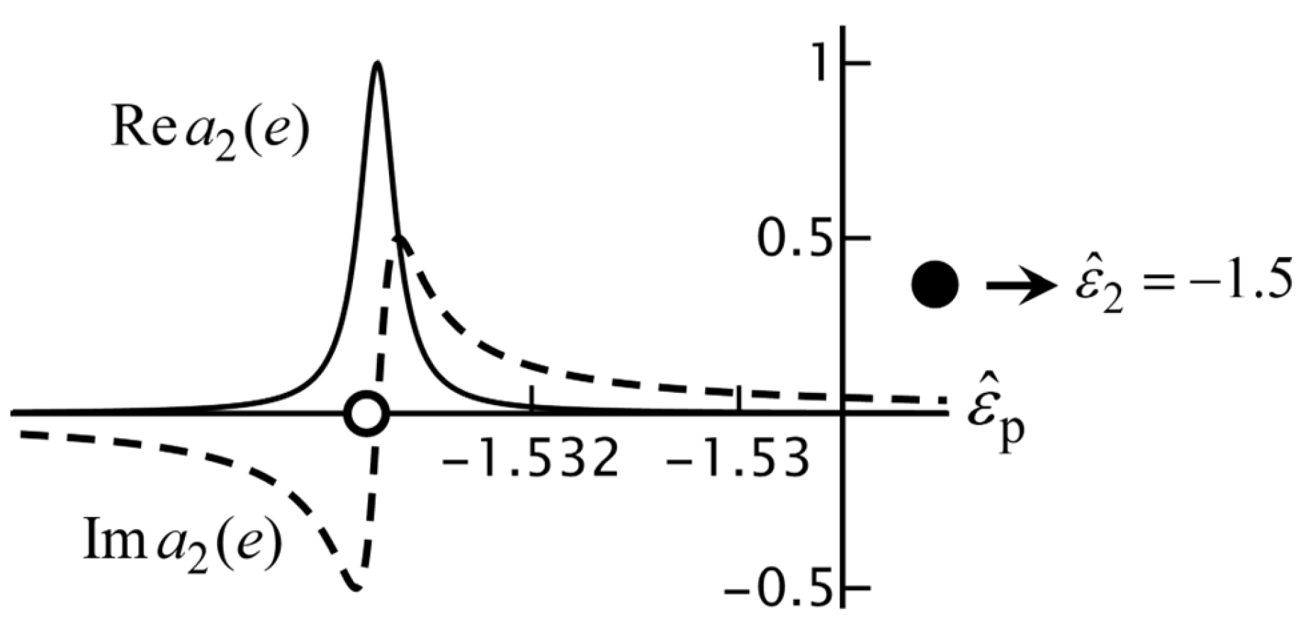
which shows that the Fröhlich resonance is located at Since we have Unlike from Equation (109), always exists. Figure 26 shows the exact for . The expected peak, according to the old approximation, Equation (97), should be located at but with the new and improved approximation, it should be located at So, there is a line shift of
This shift is to a lower and it is due to the finite radius of the particle. The shift measured from the graph is whereas the estimate (122) gives . The linewidth is estimated to be
The linewidth found from the graph is whereas Equation (123) predicts . The estimates for the shift and the width seem reasonably accurate, especially since the radius of the particle is not really small. The linewidth decreases rapidly with increasing as is illustrated in Figure 27. We also see that the original expectation of the line position is way outside the graph on the right. This is an example of the serious improvement with the new small- approximation. For the estimated values of the width and the shift, we find that the estimated shift has an error of whereas the linewidth has an error of
13. Conclusions
We have studied the Mie scattering coefficients and the Mie particle coefficients with a particular emphasis on their dependence on the (dimensionless) particle radius Central to this discussion is the Mie circle in the complex plane. When there is no dissipation in the particle or the embedding medium, then the scattering coefficients lie on this circle. We have shown this from the explicit expressions for the Mie scattering coefficients, but it can be shown that it is a direct consequence of conservation of energy in the system. For , we have . With increasing the Mie coefficients rotate around this circle. This rotation can be clockwise or counterclockwise, depending on the parameters. It is also possible that the rotation starts counterclockwise and ends clockwise. In this case, there has to be a turning point. We have presented a numerical method for the evaluation of this turning point. When there is absorption in the particle and not in the host medium, the curve in the complex plane bends to the inside of the Mie circle, and for large , the Mie scattering coefficients rotate clockwise around a smaller circle. We have derived an expression for the radius of this reduced Mie circle. When there is absorption in the host medium and not in the particle, the magnitudes of the Mie coefficients increase exponentially with the particle radius
A particularly interesting phenomenon is the Fröhlich resonance for a small particle. When the relative permittivity of the particle is in the neighborhood of with the order of the multipole, then the electric multipole Mie coefficient has a resonance. In the usual approximation of for small Equation (47), we get a division by zero, which is unphysical. We have shown that a more careful approximation formula for small gives at the resonance. Our approximation also puts on the Mie circle, which guarantees conservation of energy. The dependence of has the form of a resonance line. We have derived expressions for the position and width of this line, based on the small- approximation, and this was numerically found to be in excellent agreement with the exact result for the Mie coefficients. Also, the dependence on has the appearance of a resonance line.
Funding
This research received no external funding.
Data Availability Statement
No new data were created or analyzed in this study. Data sharing is not applicable to this article.
Conflicts of Interest
The author declares no conflicts of interest.
Appendix A
Multipole Fields
In this Appendix we present the representations of the various fields in terms of the vector spherical harmonics. The vector spherical harmonics are defined as [28,29,30]
Here, is a (scalar) spherical harmonic, is a spherical unit vector, and is a Clebsch–Gordan coefficient. The values are and given the range of values is Given we have as possible values, except that for , we only have . This set of vector spherical harmonics is a complete, orthonormal set of vector functions on the unit sphere. The definition (A1) may seem cumbersome, but when worked out in terms of the spherical-coordinate unit vectors and , the resulting expressions are quite attractive [31].
The incident electric field can be expanded as [21] (p. 471)
The parameter is defined as
and is a spherical Bessel function. The curl can be evaluated in terms of the vector spherical harmonics as
where is any spherical Bessel function. Only vector spherical harmonics with appear, which represents the polarization of the incident field. Also, the lowest value is . Due to the orthogonality of the vector spherical harmonics, the scattered and particle fields can only have and The expansion of the incident magnetic field follows from multiplying by according to Equation (20).
The scattered fields are expanded as
Here, is a spherical Hankel function. The only unknowns in these expressions are the Mie scattering coefficients and We have split off several factors, like and in order to maximize the symmetry between both Mie coefficients. Also, in this way, the Mie coefficients are independent of the laser polarization When other polarizations are needed, obtained by superposition, then this does not affect the Mie coefficients.
Similarly, the fields inside the particle are represented as
The unknowns here are the Mie particle coefficients and We have split off the factors and which will appear to be advantageous, as shown in Appendix B.
Appendix B
Boundary Conditions and Mie Coefficients
In this Appendix we outline how the Mie coefficients are computed from the boundary conditions at the surface of the sphere, so at and for all In terms of the dimensionless fields, these conditions are
It can be shown that Equations (A11) and (A12) hold when (A9) and (A10) hold, so we only need to consider the first two. We need the cross products with of all the fields from Appendix A. For the terms with the curls, we need the identity
where the value is either or We introduce the function
For the cross products involving the spherical Hankel function, we find similarly
with
For the cross product with , we have
although we shall not need this explicit result. It suffices to notice that this expression only involves and which are both orthogonal to We get, for instance,
and similarly for the other fields. Then, we set in these expressions. The boundary conditions have to hold for each separately due to orthogonality in the first Also, due to orthogonality in the middle the conditions have to hold for each term with and for each term with separately. This leads to four equations for the four unknown Mie coefficients. Two of these equations are
These equations only involve the Mie coefficients and The second set of equations relate and This set is identical to (A19) and (A20), but is replaced by in Equation (A20). Therefore, if we solve Equations (A19) and (A20) for the electric multipole coefficients, then we also have the solution for the magnetic multipole Mie coefficients. We simply make the substitution
It is advantageous to go to dimensionless variables at this point. We have and The determinant of the set is
Then, we introduce the function
We find for the Mie coefficients
The result for has been simplified with the Wronski relation:
An interesting form for the Mie coefficients can be obtained as follows. We eliminate and from with
Here, is the spherical Neumann function, and we introduce
in analogy to Equations (A14) and (A16). Similar to Equation (A22), we set
Then,
and the electric multipole Mie scattering coefficient becomes
Yet another representation, which is useful for analysis, can be found as follows. With recursion relations for spherical Bessel functions, we have
After some rearrangements, we find
We then also have
We notice that follows from under the substitution and follows from under the substitution The spherical Bessel functions with argument are the same in all three functions. We also see that and only involve the spherical Bessel functions and
For the magnetic multipole fields, we have and which follow from the substitution in the corresponding electric multipole functions.
Let us do a quick consistency check. For and , the particle material matches the embedding material, so the particle is transparent. We then have and . With Equation (A34), we find and with Equation (A23), this gives . Therefore, there is no scattered radiation. With the Wronski relation,
we find from Equation (A35). Then, and with Equation (A24), this gives . With Equations (A7) and (A8), we then see that and The field inside the particle is equal to the incident field, like there is no particle.
The computation of a single Mie coefficient involves the evaluation of a large number of spherical Bessel functions. It turns out that Mathematica can compute about 5000 Mie coefficients per second. This means that the runtime for the various graphs in this paper, which involve Mie coefficients, is about one second. Of course, this depends somewhat on the parameters and the range.
Appendix C
Dipole Fields
When a dielectric particle is small compared to the wavelength of the incident radiation, then the electric dipole term () will be the dominant radiation mode. For a metallic particle, the magnetic dipole contribution () becomes comparable to the electric dipole field [21] (p. 459). In this Appendix, we shall consider the scattered dipole fields and show the connection with the expressions for the dipole radiation of a point particle at the origin of coordinates. We shall not make any assumptions about the radius of the particle.
The scattered electric and magnetic fields are given by Equations (A5) and (A6). The dipole contributions are the terms, and it can be seen from the Mie coefficients which parts are the electric and magnetic dipole contributions. For an electric dipole, we have
and for a magnetic dipole, we have
For the curls, we use Equation (A4) with
These fields contain the vector spherical harmonics:
With , we find for the electric dipole fields
and with , we find for the magnetic dipole fields
Here, we have temporarily set to keep the equations somewhat compact.
On the other hand, if a point particle at the origin of coordinates has an oscillating electric dipole moment with a complex amplitude so that
then this particle will emit electric dipole radiation. The emitted fields are, when expressed in spherical Hankel functions [21] (pp. 411, 413),
Similarly, an oscillating magnetic dipole moment emits the fields
When we compare the expressions for the fields from Mie theory with the expressions of the fields for and we identify
These are the electric and magnetic dipole moments that are induced by the laser beam in the Mie particle. The dipole fields outside the sphere are then identical to the fields of a point particle at the origin of coordinates with the dipole moments and These induced dipole moments are proportional to the corresponding Mie coefficients. The complex amplitude is proportional to It follows from Equation (A50) that the dipole moment has the magnitude
which is independent of time. It rotates in the plane, and for , the rotation is counterclockwise when viewed down the positive axis. This is the same direction of rotation as the electric incident field for a given point in space. The same holds for The incident fields at the center of the particle are
The dipole moments are induced by the incident fields, and with Equations (A55) and (A56), we see that
The electric and magnetic polarizabilities and are defined, in general, as
and so we find
This shows that the polarizabilities are determined entirely by the corresponding dipole Mie scattering coefficients. Many authors define as Although this is an equally acceptable definition, it destroys the symmetry between electric and magnetic dipoles.
A convenient dimensionless representation of the polarizabilities is by means of the polarizability volumes:
By combination of the above formulas, we then find
In the scattered fields, Equations (A46)–(A49), we can eliminate and in favor of the polarizability volumes.
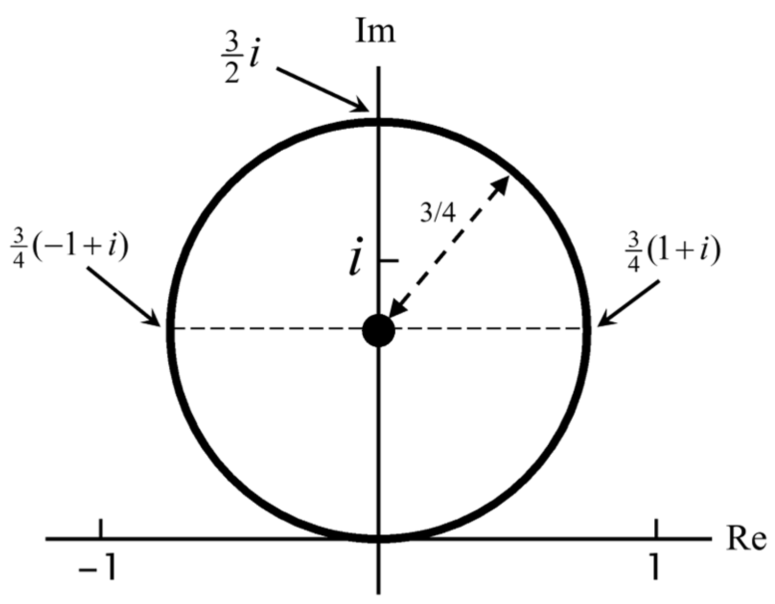
When there is no dissipation in the system, then lies on the Mie circle, as shown in Section 4. It then holds that and with Equation (A68), this implies
This represents a circle in the complex plane with radius 3/4, around 3i/4. We call this the polarizability circle [32], and this circle is shown in Figure A1. It can be shown that the polarizability of a particle must lie on this circle when there is no dissipation in the system. This does not only hold for a Mie particle but also in general.
Figure A1.
The figure shows the polarizability circle.
Appendix D
Dipole Mie Coefficients
For dipoles, the Mie coefficients can be expressed in terms of elementary functions. For this we need
We set in Equations (A34) and (A35), to find and and with Equation (A30), we find After some regrouping, we then find for the electric dipole
with
For a magnetic dipole, we replace
It may seem that these formulas are bigger than the expressions for the general Mie coefficients. It should be noted, however, that the results from this section only involve sines and cosines, which are much easier to evaluate numerically. It turns out that the expressions given here for dipoles are about 15 times faster, numerically, than the general expressions with . It also appears that the results above are numerically much more stable.
Appendix E
Perfect Conductor
For a metallic particle, the fields, charges and currents are mainly present in the region just inside the surface of the sphere. For a perfectly conducting sphere, all charges and currents are confined to the surface, and there are no fields inside the particle. So, we have
The surface charge density and the surface current density appear in the boundary conditions as
with the electric and magnetic fields evaluated just outside the surface. One immediate consequence is that the boundary condition (A10), which was used in the derivation of the Mie coefficients, does not apply for a perfect conductor. Similarly, condition (A11) does not hold here. So, we are left with
The right-hand sides are zero due to Equation (A77). It is sometimes stated in the literature [19] that the limit of a perfect conductor follows by letting , but that is not correct in general. This point was also made in [33], where it was shown that this limit would give non-zero fields inside the particle.
In Appendix B we used the cross products of with vector spherical harmonics (Equations (A13) and (A17)). Due to condition (A81), we now also need the dot product of with vector spherical harmonics. These are
with any spherical Bessel function. Along the same lines as in Appendix B, we now find for the Mie scattering coefficients
with and defined by Equations (A14) and (A16), respectively. For a perfect conductor, there is no symmetry between the electric and magnetic Mie scattering coefficients. The results (A84) and (A85) can also be written as
with defined by Equation (A28). In this form, they have the same appearance as the general Mie coefficients in Equation (21), and we could identify the functions and for a perfect conductor.
Just as in Appendix D, the spherical Bessel functions can be eliminated in favor of simpler functions for dipoles. For a perfectly conducting electric dipole, we find
with and for a magnetic dipole, we have
Appendix F
Derivatives of the Mie Scattering Coefficients
In order to find the turning points of the Mie scattering coefficients on the Mie circle, we need the derivatives of the Mie coefficients with respect to the radius of the particle. With the representation (21), we have
Therefore, we need the derivatives of the functions and which are given by Equations (A34) and (A35) for This may seem a monumental task due to the appearance of the numerous spherical Bessel functions. Derivatives of spherical Bessel functions can be eliminated with recursion relations. It appears that many terms cancel, and the final result is quite attractive. We obtain for the electric multipole Mie coefficients
The function is given by Equation (A32). One may wonder how the parameter enters this expression because this parameter does not appear in the functions and It comes from combining several terms with the help of the identity
The corresponding expression for the magnetic multipole Mie coefficient follows by exchanging
Of particular importance is the case . Equation (A91) simplifies to
and the result for magnetic multipoles simplifies even more:
For a perfect conductor, we need to redo the computation, since this case does not correspond to a limit of the general result. Differentiating Equations (A86) and (A87) yields
Equation (A95) will be of help when studying the turning points on the Mie circle for a metallic particle.
References
- Mie, G. Beiträge zur Optik trüber Medien, speziell kolloidaler Metallösungen. Ann. Der Phys. 1908, 25, 377–455. [Google Scholar] [CrossRef]
- Zhao, Q.; Zhou, J.; Zhang, F.; Lippens, D. Mie resonance-based dielectric metamaterials. Mater. Today 2009, 12, 60–69. [Google Scholar] [CrossRef]
- Kuznetsov, A.I.; Miroshnichenko, A.E.; Brongersma, M.L.; Kivshar, Y.S.; Luk’yanchuk, B. Optically resonant dielectric nanostructures. Science 2016, 354, aag2472. [Google Scholar] [CrossRef] [PubMed]
- Kivshar, Y. The rise of Mie-tronics. Nano Lett. 2022, 22, 3513–3515. [Google Scholar] [CrossRef]
- Devilez, A.; Stout, B.; Bonod, N.; Popov, E. Spectral analysis of three-dimensional photonic jets. Opt. Exp. 2008, 16, 14200–14212. [Google Scholar] [CrossRef]
- Lecier, S.; Perrin, S.; Leong-Hoi, A.; Montgomery, P. Photonic jet lens. Sci. Rep. 2019, 9, 4725. [Google Scholar]
- Chýlek, P. Asymptotic limits of the Mie-scattering characteristics. J. Opt. Soc. Am. 1975, 65, 1316–1318. [Google Scholar] [CrossRef]
- Wiscombe, W.J. Improved Mie scattering algorithms. Appl. Opt. 1980, 19, 1505–1509. [Google Scholar] [CrossRef] [PubMed]
- Shore, R.A. Scattering of an electromagnetic linearly polarized plane wave by a multilayered sphere. IEEE Antennas Propag. 2015, 57, 69–116. [Google Scholar] [CrossRef]
- Grigoriev, V.; Bonod, N.; Wenger, J.; Stout, B. Optimizing nanoparticle design for ideal absorption of light. ACS Photonics 2015, 2, 263–270. [Google Scholar] [CrossRef]
- Tribelsky, M.I. Phenomenological approach to light scattering by small particles and directional Fano’s resonances. EPL 2013, 104, 34002. [Google Scholar] [CrossRef]
- Tzarouchis, D.C.; Ylä-Oijala, P.; Sihvola, A. Unveiling the scattering behavior of small spheres. Phys. Rev. B 2016, 94, 140301. [Google Scholar] [CrossRef]
- Jia, X. Calculation of auxiliary functions related to Riccati-Bessel functions in Mie scattering. J. Mod. Opt. 2016, 63, 2348–2355. [Google Scholar] [CrossRef]
- Colom, R.; Devilez, A.; Bonod, N.; Stout, B. Optimal interactions of light with magnetic and electric resonant particles. Phys. Rev. B 2016, 93, 045427. [Google Scholar] [CrossRef]
- Tzarouchis, D.; Sihvola, A. Light scattering by a dielectric sphere: Perspective on Mie resonances. Appl. Sci. 2018, 8, 184. [Google Scholar] [CrossRef]
- Guidet, C.-H.; Stout, B.; Abdedaim, R.; Bonod, N. Poles, physical bounds, and optimal materials predicted with approximated Mie coefficients. J. Opt. Soc. Am. B 2021, 38, 979–989. [Google Scholar] [CrossRef]
- Tribelsky, M.I.; Miroshnichenko, A.E. Resonant scattering of electromagnetic waves by small particles: A new insight into the old problem. Phys.-Uspekhi 2022, 65, 40–61. [Google Scholar] [CrossRef]
- van de Hulst, H.C. Light Scattering by Small Particles; Wiley: Hoboken, NJ, USA, 1957. [Google Scholar]
- Kerker, M. The Scattering of Light; Academic Press: Cambridge, MA, USA, 1969. [Google Scholar]
- Bohren, C.F.; Huffman, D.R. Absorption and Scattering of Light by Small Particles; Wiley: Hoboken, NJ, USA, 1983. [Google Scholar]
- Jackson, J.D. Classical Electrodynamics; Wiley: Hoboken, NJ, USA, 1998. [Google Scholar]
- Chew, H.; McNulty, P.J.; Kerker, M. Model for Raman and fluorescent scattering by molecules embedded in small particles. Phys. Rev. A 1976, 13, 396–404. [Google Scholar] [CrossRef]
- Kerker, M. Lorenz-Mie scattering by spheres: Some newly recognized phenomena. Aerosol Sci. Technol. 1982, 1, 275–291. [Google Scholar] [CrossRef]
- Arnoldus, H.F. The Mie circle. Opt. Commun. 2023, 537, 129357. [Google Scholar] [CrossRef]
- Arnoldus, H.F. Energy flow in light scattering by a small conducting sphere. J. Appl. Phys. 2023, 133, 114304. [Google Scholar] [CrossRef]
- Arnoldus, H.F. Mie scattering near the Fröhlich mode. J. Opt. Soc. Am. A 2025, 42, 580–586. [Google Scholar] [CrossRef]
- Tribelsky, M.I.; Luk’yanchuk, B.S. Anomalous light scattering by small particles. Phys. Rev. Lett. 2006, 97, 263902. [Google Scholar] [CrossRef] [PubMed]
- Eisenberg, J.M.; Greiner, W. Excitation Mechanisms of the Nucleus; North-Holland: Amsterdam, The Netherlands, 1975. [Google Scholar]
- Weissbluth, M. Atoms and Molecules; Academic Press: Cambridge, MA, USA, 1978. [Google Scholar]
- Arfken, G.B.; Weber, H.J.; Harris, F.E. Mathematical Methods for Physicists, 7th ed.; Academic Press: Cambridge, MA, USA, 2013; p. 810. [Google Scholar]
- Hill, E.H. The theory of vector spherical harmonics. Am. J. Phys. 1954, 22, 211–214. [Google Scholar] [CrossRef]
- Arnoldus, H.F. The polarizability circle. Phys. Lett. A 2022, 428, 127923. [Google Scholar] [CrossRef]
- Tribelsky, M.I.; Miroshnichenko, A.E. Giant in-particle field concentration and Fano resonances in light scattering by high-refractive-index particles. Phys. Rev. A 2016, 93, 053837. [Google Scholar] [CrossRef]
Figure 1.
Shown is the setup for Mie scattering.

Figure 2.
Shown is the Mie circle in the complex plane. Without absorption, the Mie scattering coefficients lie on this circle. The white circle on the real axis is the Mie resonance.
Figure 2.
Shown is the Mie circle in the complex plane. Without absorption, the Mie scattering coefficients lie on this circle. The white circle on the real axis is the Mie resonance.
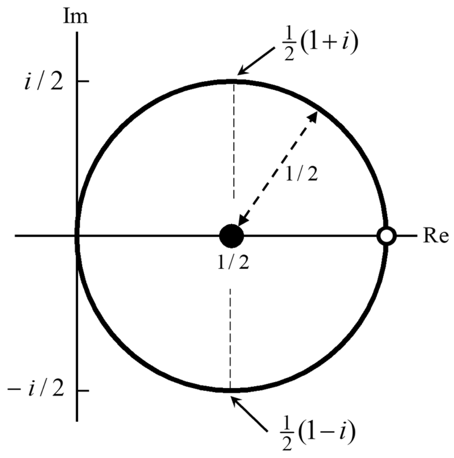
Figure 3.
The graph shows for and . The arrows indicate the direction of increasing The graph does not start at the origin for (Section 6, Equation (48)), and the maximum value of here is 4.5.
Figure 3.
The graph shows for and . The arrows indicate the direction of increasing The graph does not start at the origin for (Section 6, Equation (48)), and the maximum value of here is 4.5.
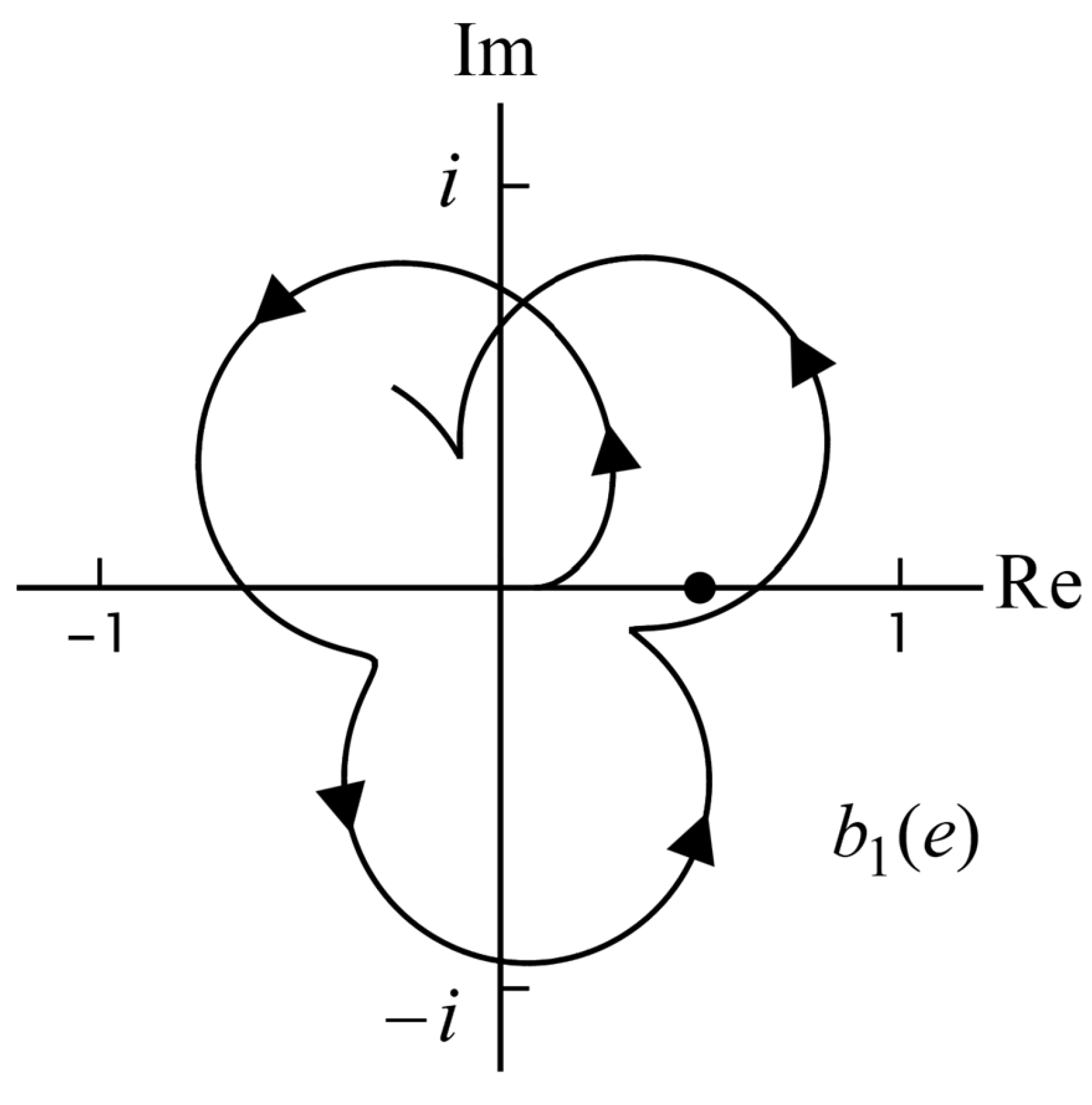
Figure 4.
The graph shows the real part of the Mie scattering coefficient for and . The solid curve represents the exact value, and the dashed curve is the asymptotic approximation for large .
Figure 4.
The graph shows the real part of the Mie scattering coefficient for and . The solid curve represents the exact value, and the dashed curve is the asymptotic approximation for large .
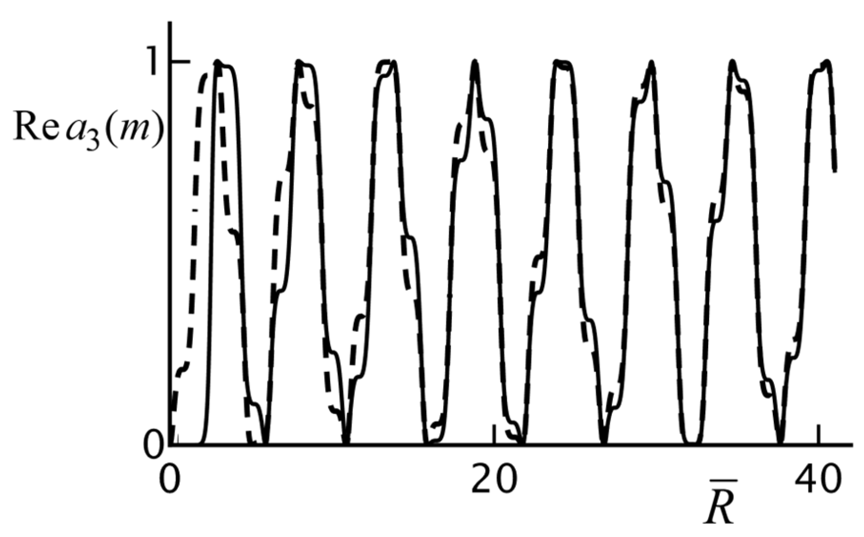
Figure 5.
The graph shows the Mie particle coefficient for and . For , we have with Equation (48), and with increasing , this Mie coefficient spirals into the origin.
Figure 5.
The graph shows the Mie particle coefficient for and . For , we have with Equation (48), and with increasing , this Mie coefficient spirals into the origin.
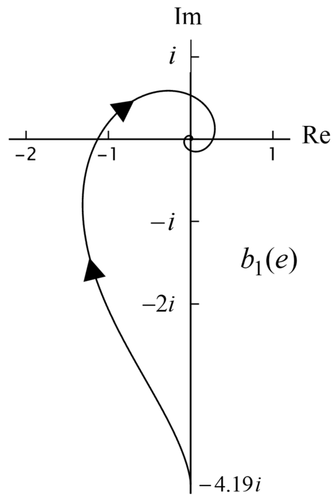
Figure 6.
The figure shows how the rotation directions of the Mie scattering coefficients over the Mie circle, with increasing depend on the parameter .
Figure 6.
The figure shows how the rotation directions of the Mie scattering coefficients over the Mie circle, with increasing depend on the parameter .
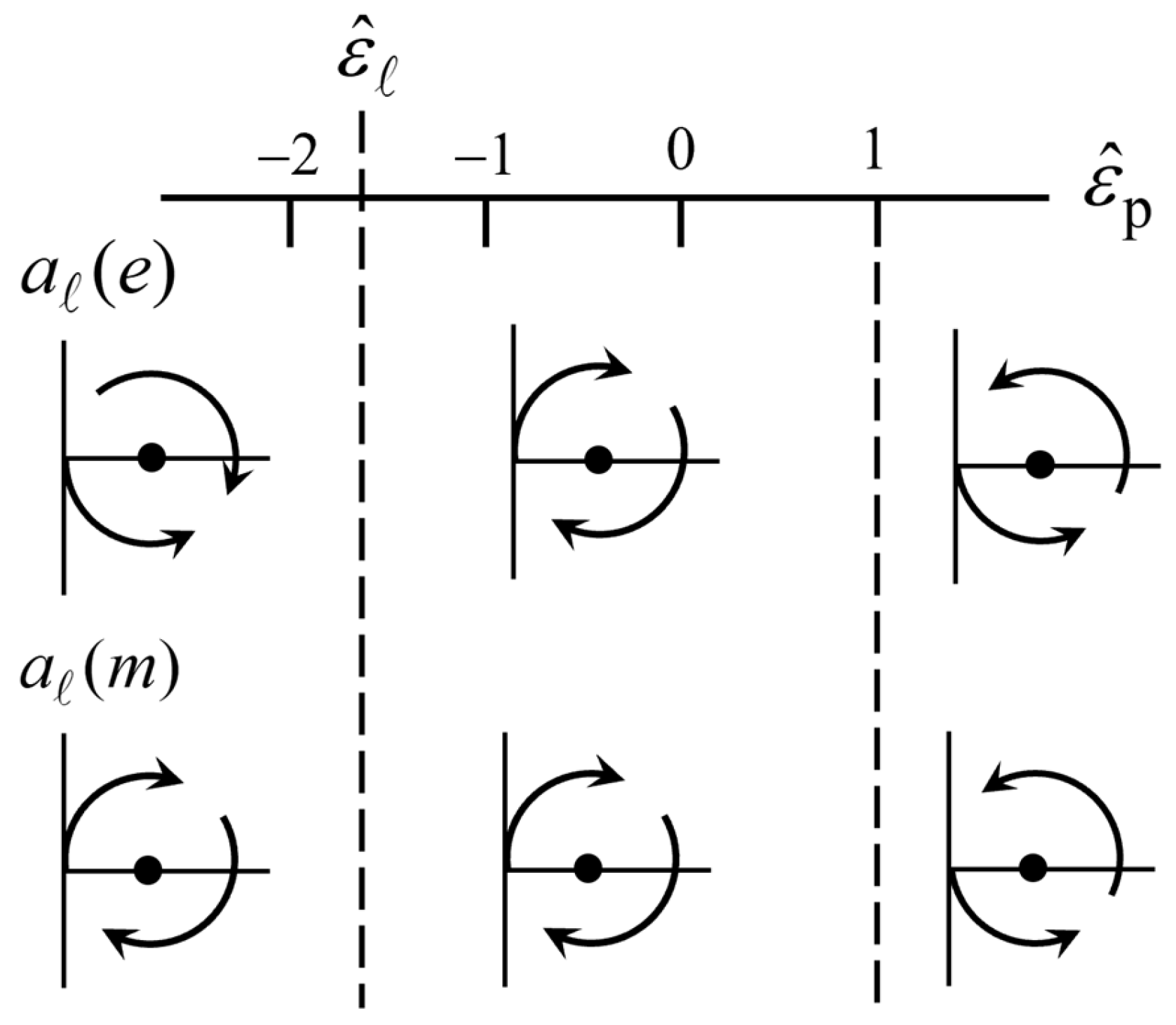
Figure 7.
The figure shows how the rotation directions of the Mie particle coefficients around the origin, with increasing depend on the parameter The three black dots indicate the values for . For the curves start on the positive real axis, and for , they can start anywhere on an axis.
Figure 7.
The figure shows how the rotation directions of the Mie particle coefficients around the origin, with increasing depend on the parameter The three black dots indicate the values for . For the curves start on the positive real axis, and for , they can start anywhere on an axis.
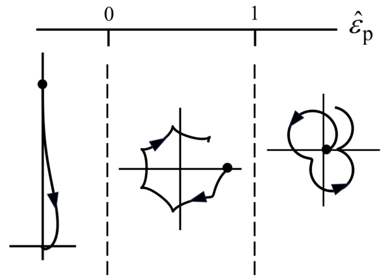
Figure 8.
Shown is the Mie scattering coefficient for and . The arrowheads indicate the direction of increasing At the white circle, the curve has a turning point, and numerically it is found to be . The dashed curve for the clockwise rotation has been displaced slightly.
Figure 8.
Shown is the Mie scattering coefficient for and . The arrowheads indicate the direction of increasing At the white circle, the curve has a turning point, and numerically it is found to be . The dashed curve for the clockwise rotation has been displaced slightly.
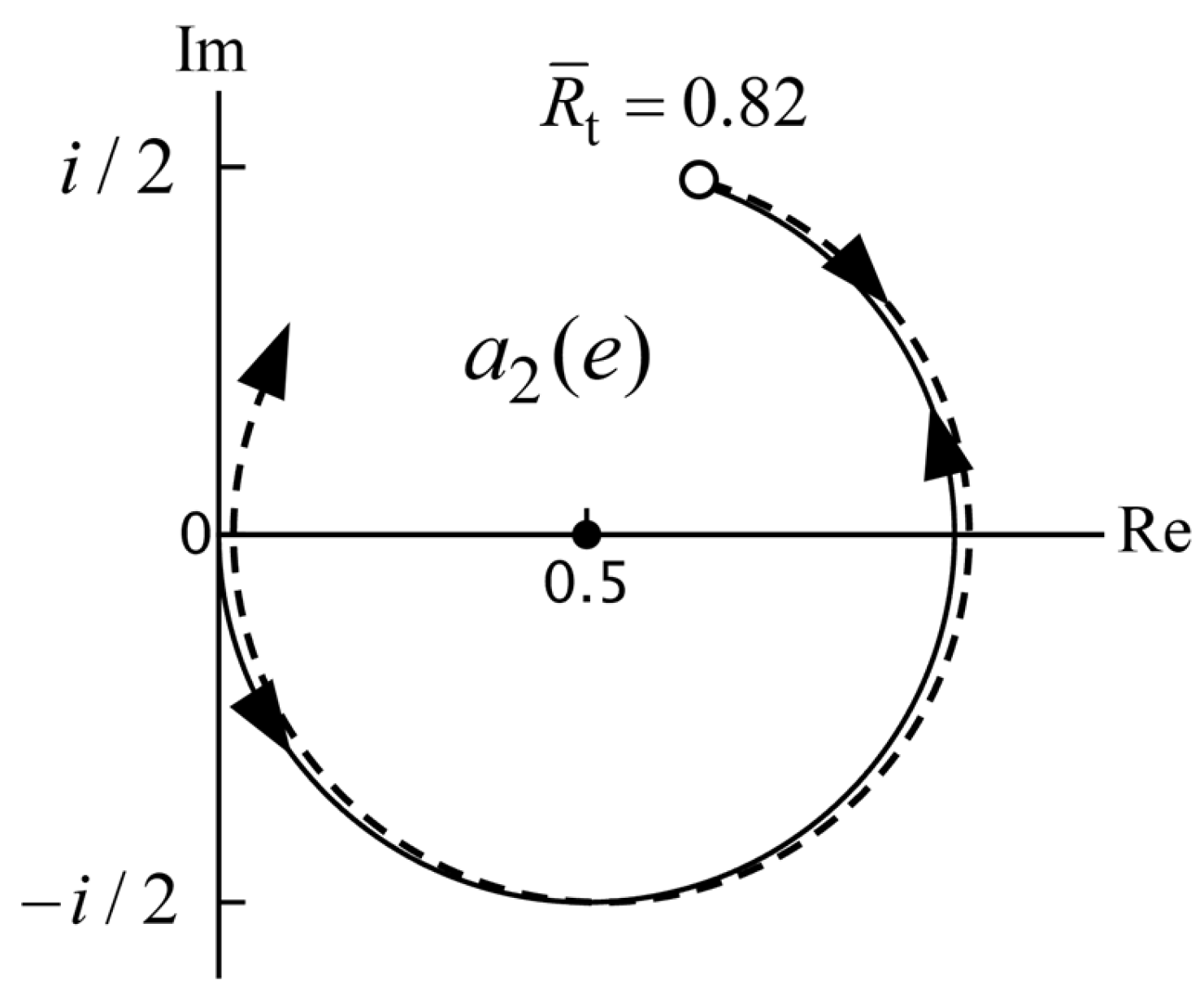
Figure 9.
The figure shows the real (solid curve) and imaginary (dashed curve) parts of the derivative of the Mie scattering coefficient as a function of and for and . At the white circle, both the real and imaginary parts vanish, and so this is the turning point .
Figure 9.
The figure shows the real (solid curve) and imaginary (dashed curve) parts of the derivative of the Mie scattering coefficient as a function of and for and . At the white circle, both the real and imaginary parts vanish, and so this is the turning point .

Figure 10.
Shown is the function seen as a function of for and as well as for three values. The white circles are the turning points .
Figure 10.
Shown is the function seen as a function of for and as well as for three values. The white circles are the turning points .
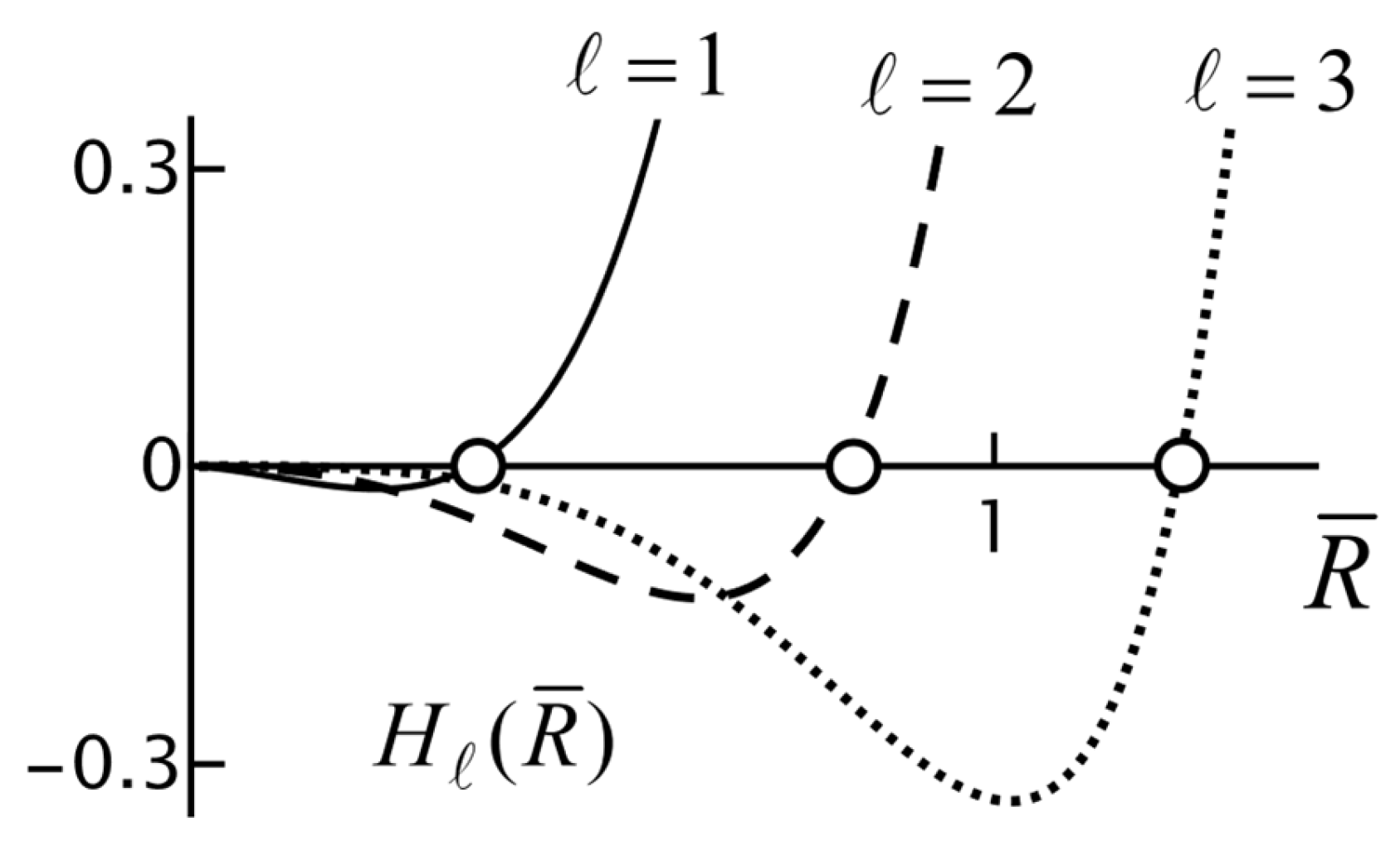
Figure 11.
The figure shows the rotation directions of the Mie scattering coefficients for the case that there is damping in the particle. The dashed arrows indicate a reversal of the rotation direction, compared to the case without damping.
Figure 11.
The figure shows the rotation directions of the Mie scattering coefficients for the case that there is damping in the particle. The dashed arrows indicate a reversal of the rotation direction, compared to the case without damping.
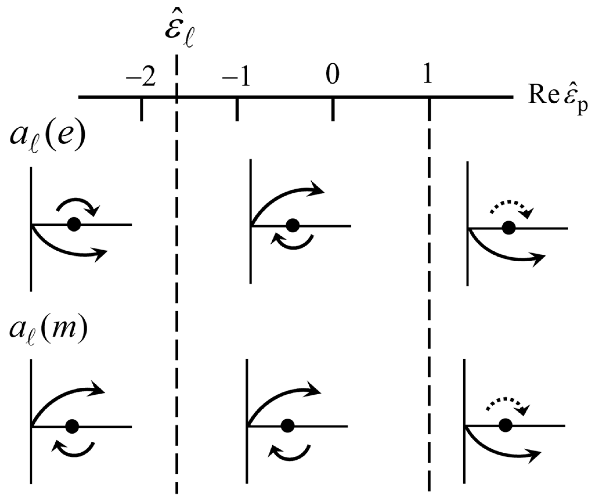
Figure 12.
The figure shows the Mie scattering coefficient for and . The curve stops at . The rotation direction is clockwise for all The dashed circle is the reduced Mie circle with a radius and for large, the Mie coefficient approaches this circle.
Figure 12.
The figure shows the Mie scattering coefficient for and . The curve stops at . The rotation direction is clockwise for all The dashed circle is the reduced Mie circle with a radius and for large, the Mie coefficient approaches this circle.
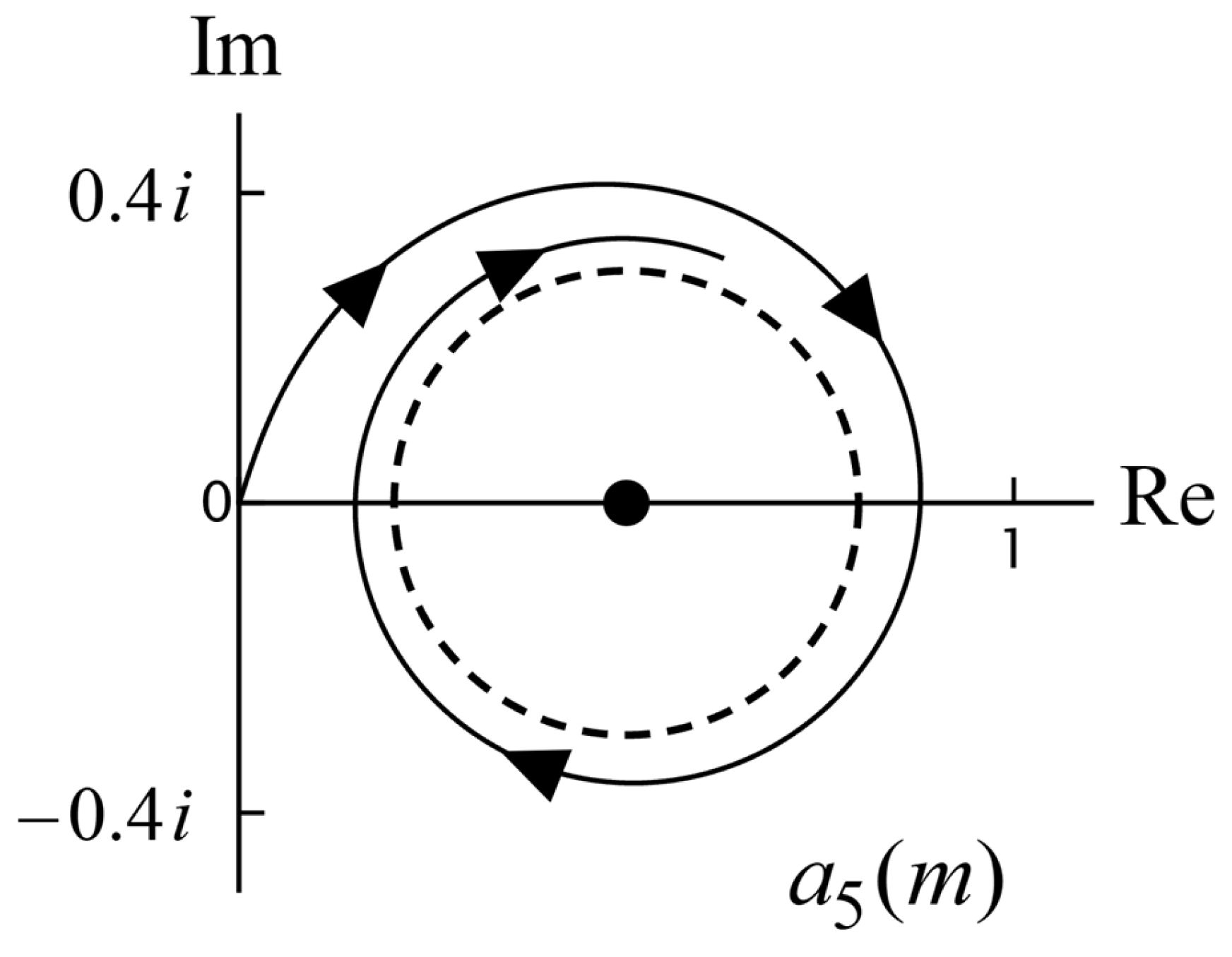
Figure 13.
Shown is the Mie scattering coefficient for and . The curve runs to . The rotation direction starts counterclockwise and ends clockwise. The dashed circle is the reduced Mie circle with a radius .
Figure 13.
Shown is the Mie scattering coefficient for and . The curve runs to . The rotation direction starts counterclockwise and ends clockwise. The dashed circle is the reduced Mie circle with a radius .
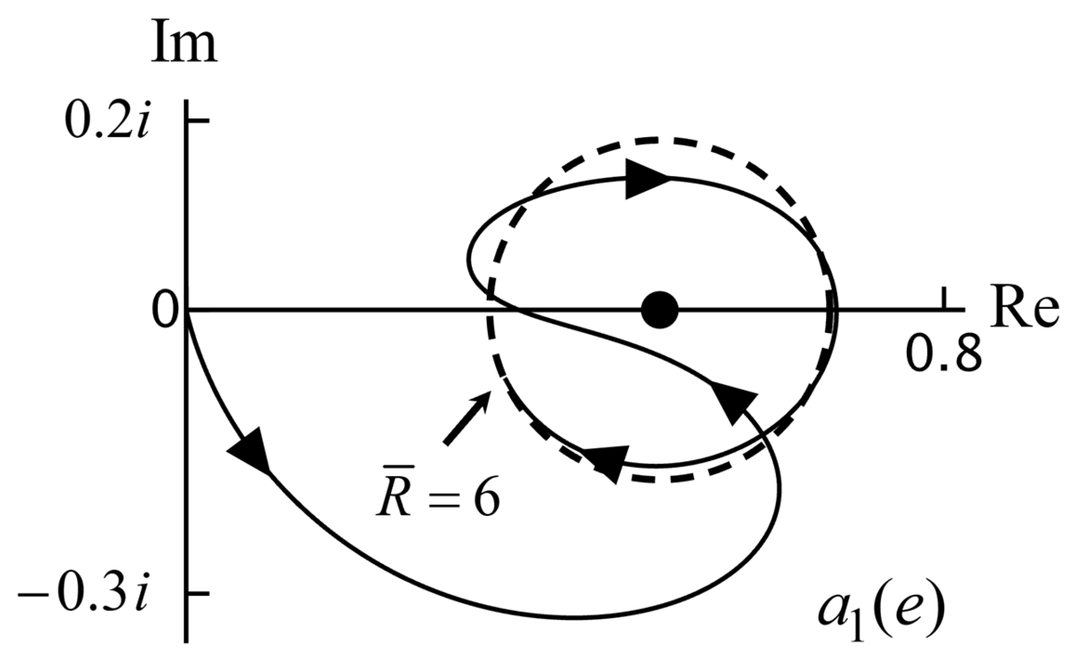
Figure 14.
The figure shows the Mie scattering coefficient for the same material parameters as in Figure 13. Here, we can clearly see the turning point, which is a result of the damping.
Figure 14.
The figure shows the Mie scattering coefficient for the same material parameters as in Figure 13. Here, we can clearly see the turning point, which is a result of the damping.
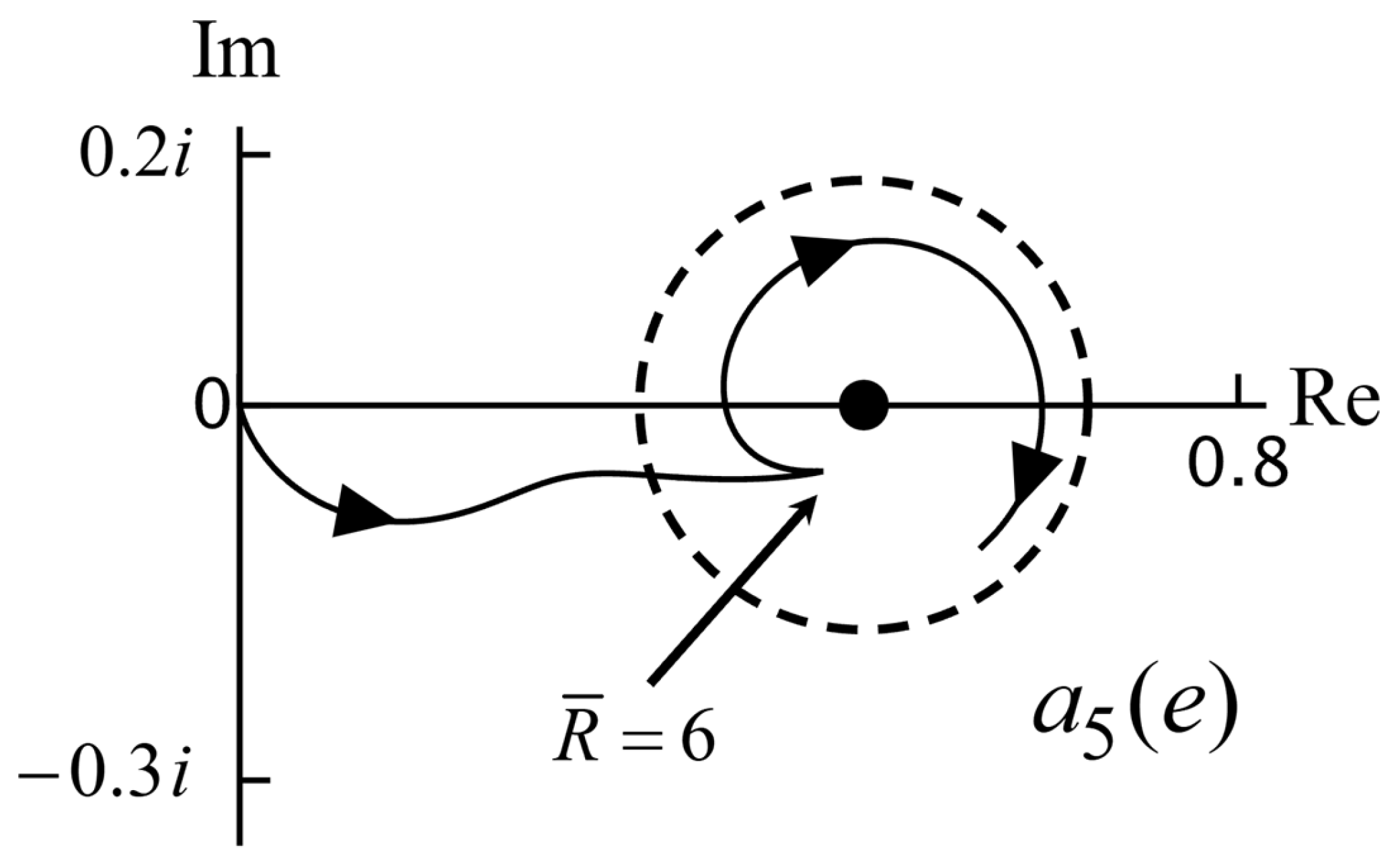
Figure 15.
The figure shows the Mie particle coefficient for the same material parameters as in Figure 13. We have and so This gives a counterclockwise rotation.
Figure 15.
The figure shows the Mie particle coefficient for the same material parameters as in Figure 13. We have and so This gives a counterclockwise rotation.
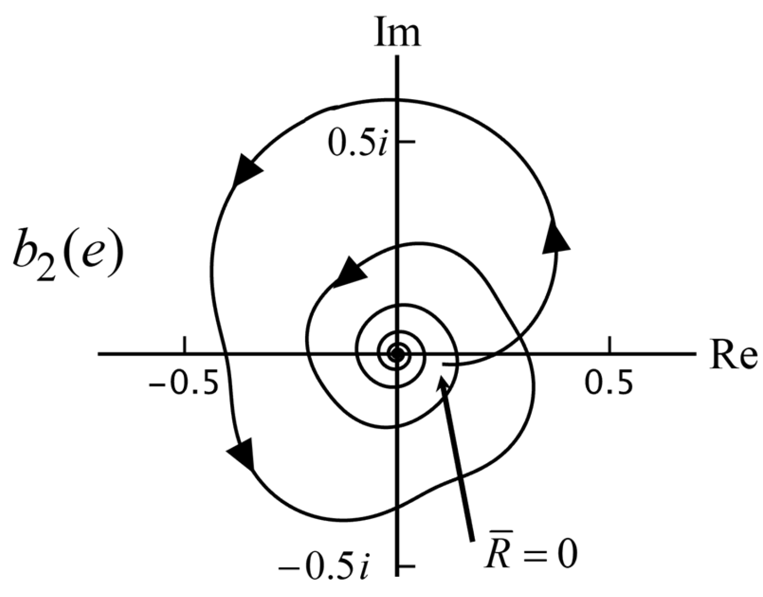
Figure 16.
The figure shows the Mie scattering coefficient for and . The indices of refraction are and . We have and this gives a counterclockwise rotation. The dashed circle is the Mie circle. With increasing the magnitude of the Mie coefficient increases exponentially.
Figure 16.
The figure shows the Mie scattering coefficient for and . The indices of refraction are and . We have and this gives a counterclockwise rotation. The dashed circle is the Mie circle. With increasing the magnitude of the Mie coefficient increases exponentially.
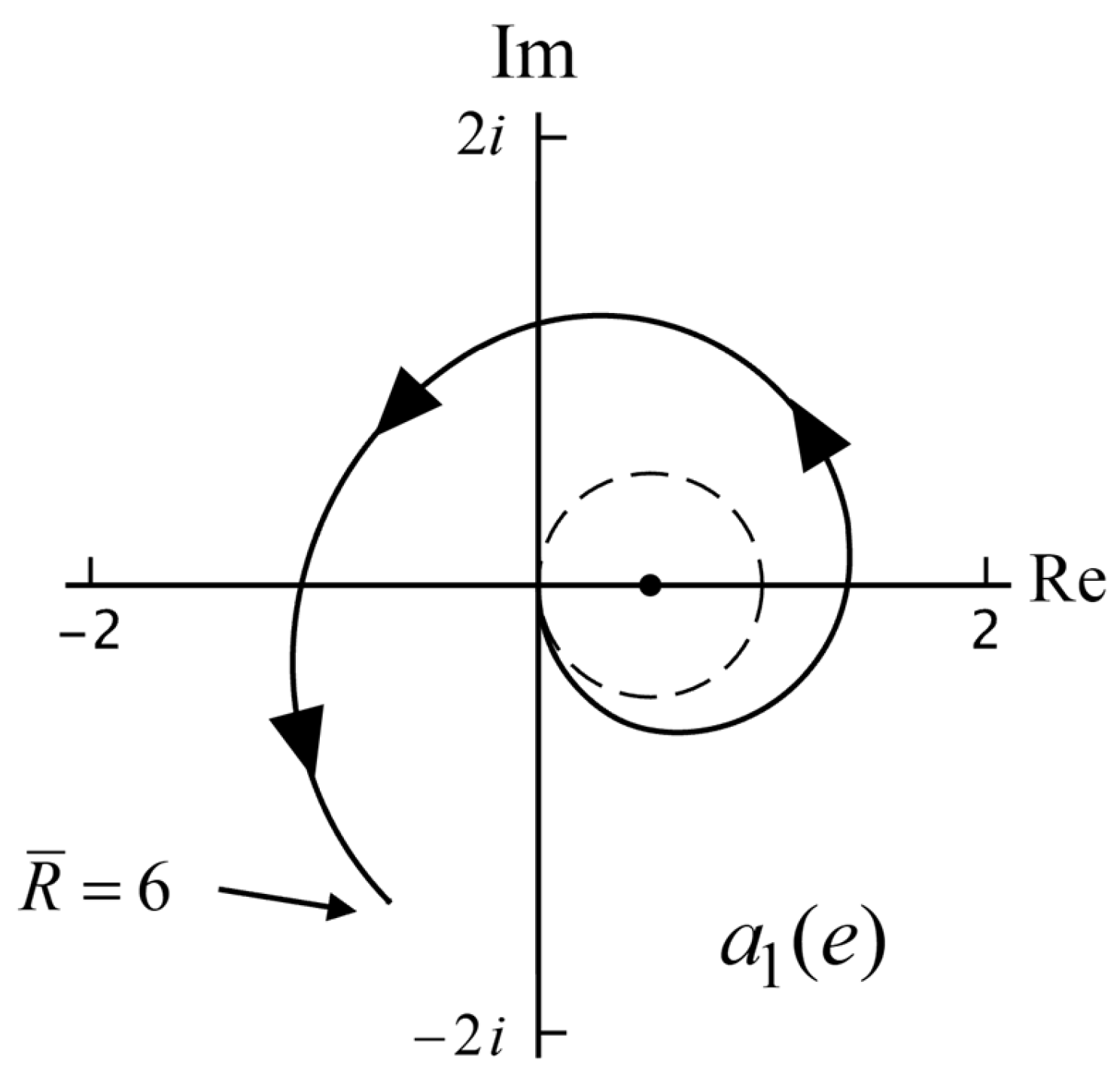
Figure 17.
The figure shows the Mie particle coefficient for and . The indices of refraction are and . We have and this gives a clockwise rotation. With increasing the magnitude of the Mie coefficient increases exponentially.
Figure 17.
The figure shows the Mie particle coefficient for and . The indices of refraction are and . We have and this gives a clockwise rotation. With increasing the magnitude of the Mie coefficient increases exponentially.
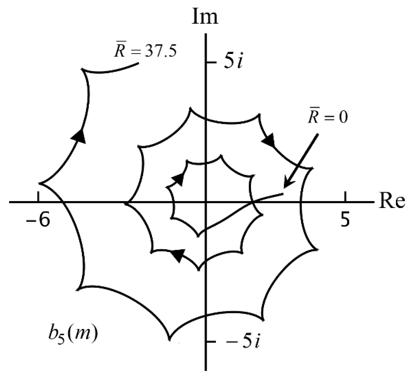
Figure 18.
Shown is for and . The indices of refraction are and so we have combined damping in the particle and the medium. We have and this gives a clockwise rotation.
Figure 18.
Shown is for and . The indices of refraction are and so we have combined damping in the particle and the medium. We have and this gives a clockwise rotation.
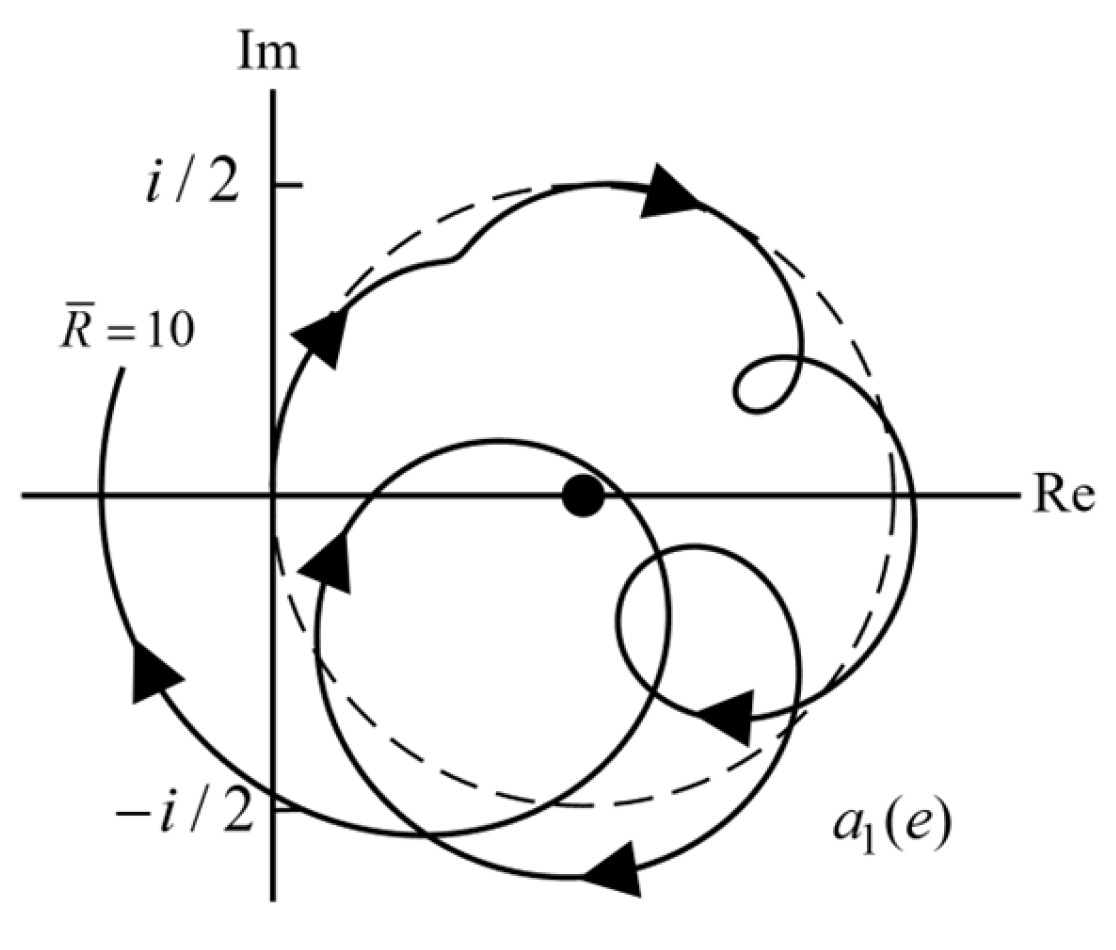
Figure 19.
The figure shows the real part of the Mie scattering coefficient (solid curve) and its small- approximation (dashed curve) for and .
Figure 19.
The figure shows the real part of the Mie scattering coefficient (solid curve) and its small- approximation (dashed curve) for and .
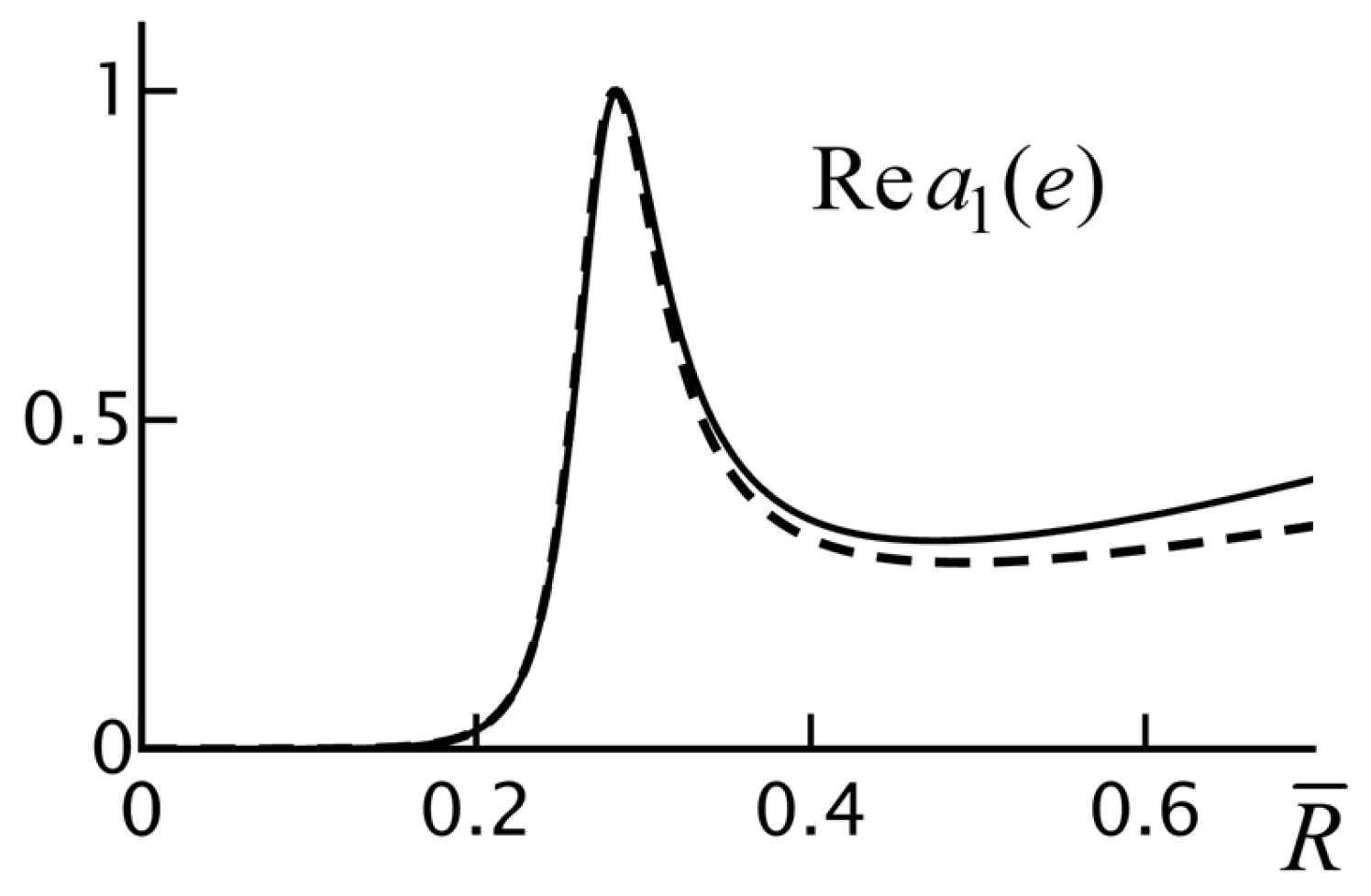
Figure 20.
The figure shows the imaginary part of the Mie particle coefficient (solid curve) and its small- approximation (dashed curve) for the same parameters as in Figure 19.
Figure 20.
The figure shows the imaginary part of the Mie particle coefficient (solid curve) and its small- approximation (dashed curve) for the same parameters as in Figure 19.
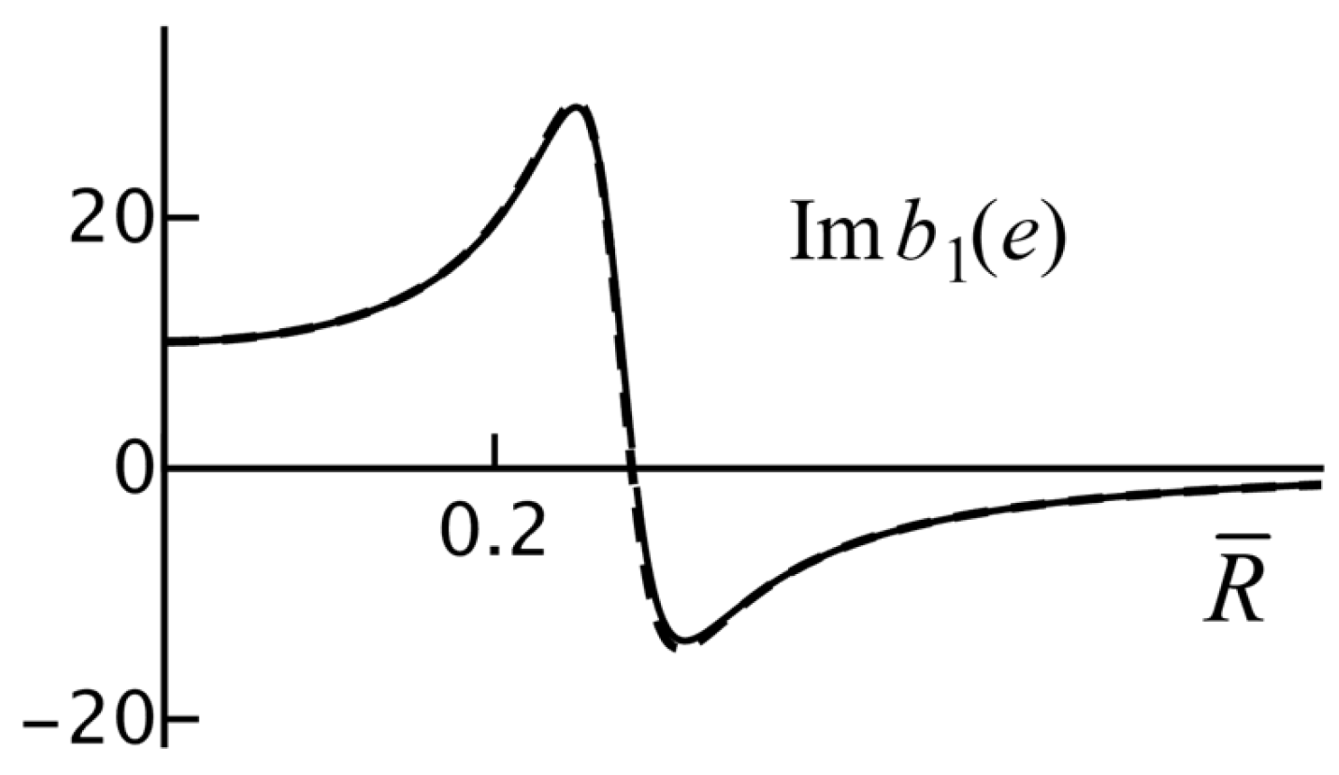
Figure 21.
The graph shows the dependence of on for . The white circle on the left is , and the white circle on the right is . The value of must lie in between these circles for to exist.
Figure 21.
The graph shows the dependence of on for . The white circle on the left is , and the white circle on the right is . The value of must lie in between these circles for to exist.
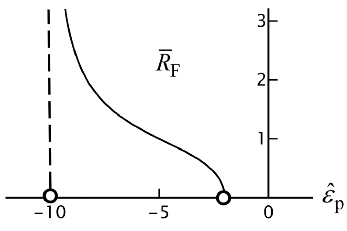
Figure 22.
The graph shows the real (solid curve) and imaginary (dashed curve) parts of as a function of for and . The vertical axis crosses the horizontal axis at . The curves are the exact values.
Figure 22.
The graph shows the real (solid curve) and imaginary (dashed curve) parts of as a function of for and . The vertical axis crosses the horizontal axis at . The curves are the exact values.
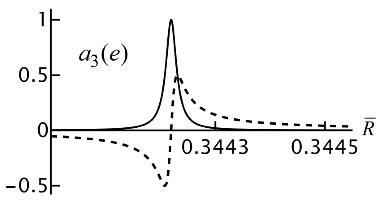
Figure 23.
The graph shows the real (solid curve) and imaginary (dashed curve) parts of as a function of for and . The spike on the left is the Fröhlich resonance. The oscillations for larger come from the rotation around the Mie circle with increasing At the left white square we have corresponding to a Mie resonance, and at the right white square we have .
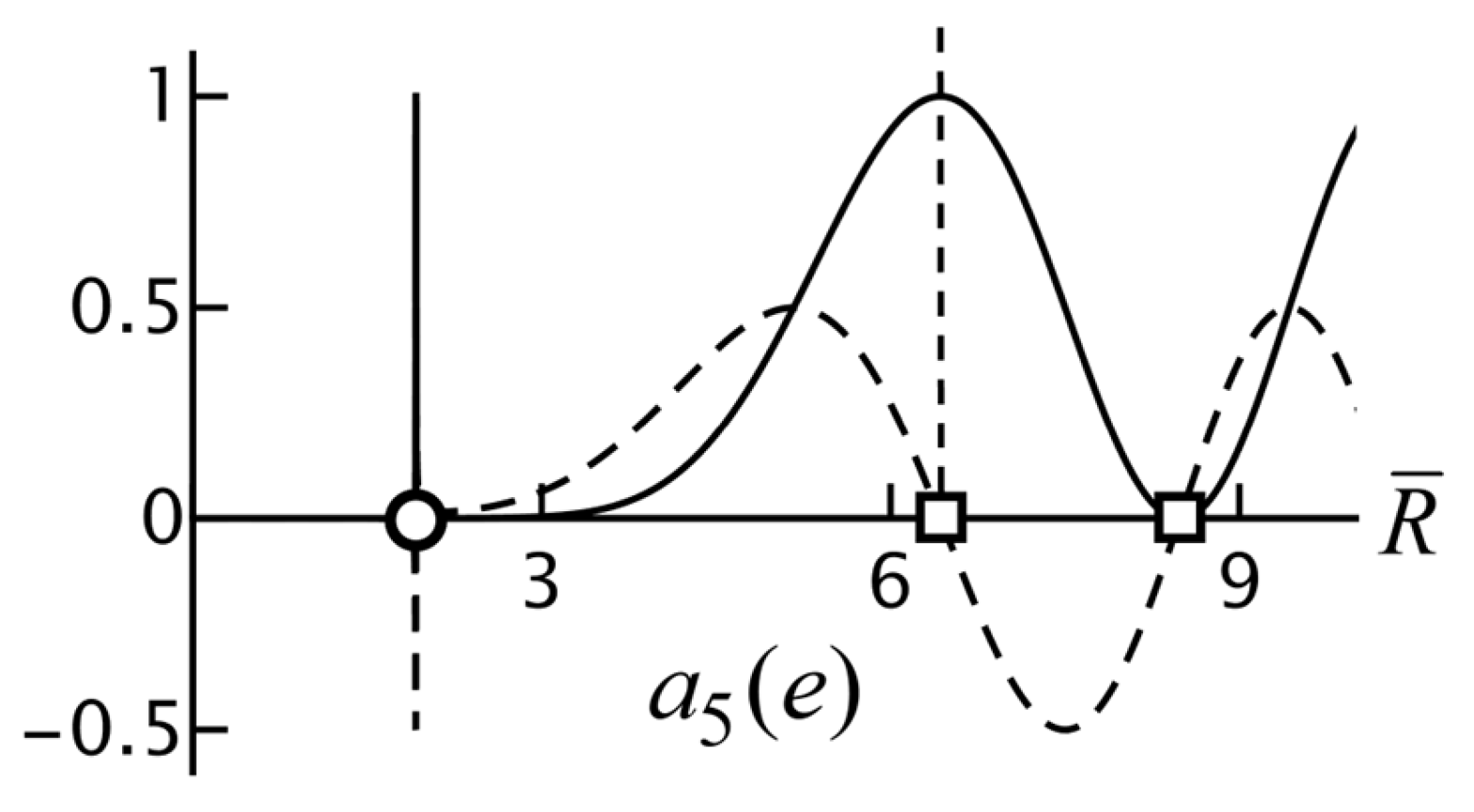
Figure 24.
The graph shows in the complex plane for and The dashed circle is the Mie circle. In between and the curve is almost a perfect circle.
Figure 24.
The graph shows in the complex plane for and The dashed circle is the Mie circle. In between and the curve is almost a perfect circle.

Figure 25.
The graph shows for and The rotation in the tiny circle is counterclockwise.
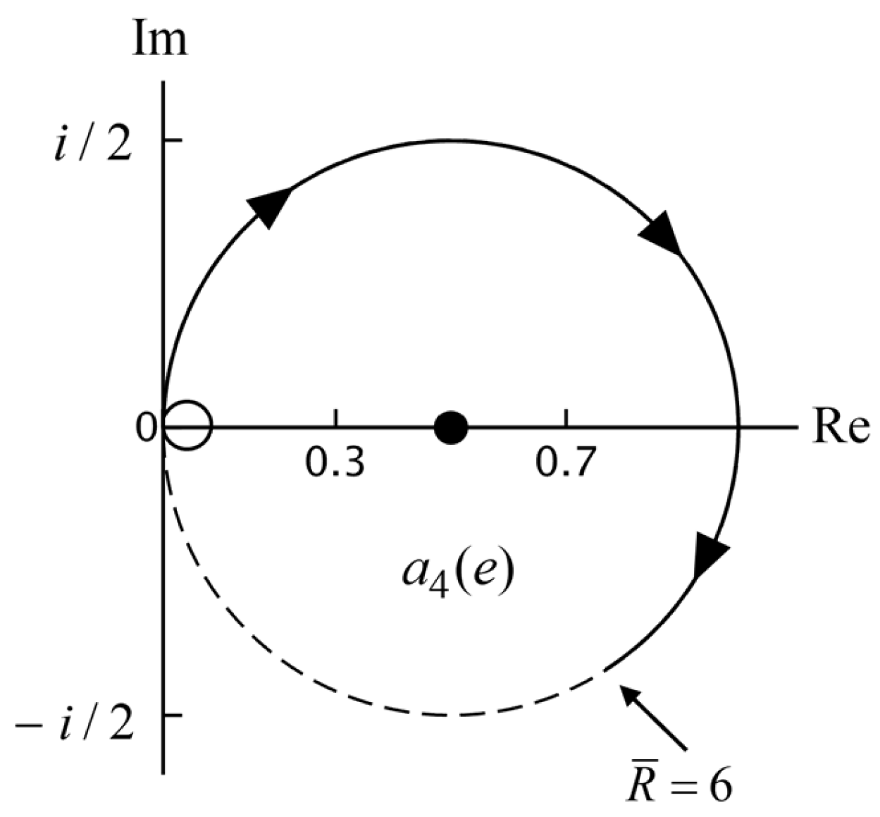
Figure 26.
The graph shows the real (solid curve) and imaginary (dashed curve) parts of as a function of for . The white circle is the value of and the black circle is . The distance between the two circles is the predicted line shift .
Figure 26.
The graph shows the real (solid curve) and imaginary (dashed curve) parts of as a function of for . The white circle is the value of and the black circle is . The distance between the two circles is the predicted line shift .
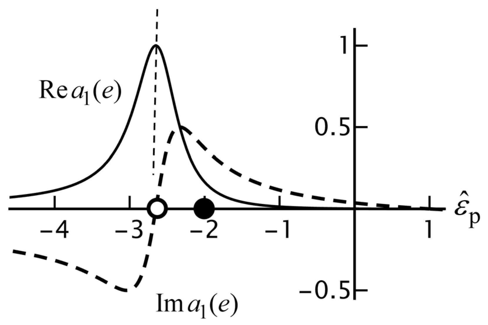
Figure 27.
The graph shows the real (solid curve) and imaginary (dashed curve) parts of as a function of for . The white circle is The vertical axis crosses the horizontal axis at .
Figure 27.
The graph shows the real (solid curve) and imaginary (dashed curve) parts of as a function of for . The white circle is The vertical axis crosses the horizontal axis at .

Table 1.
Table showing for various values of .
| 1 | 0.667 |
| 2 | 0.0333 |
| 3 | 8.47 × 10⁻⁴ |
| 4 | 1.26 × 10⁻⁵ |
| 5 | 1.22 × 10⁻⁷ |
| 10 | 1.22 × 10⁻¹⁹ |
| 20 | 2.50 × 10−49 |
Table 2.
The table shows and for various values of .
| 1 | −2.00 | −10.0 |
| 2 | −1.50 | −3.50 |
| 3 | −1.33 | −2.40 |
| 4 | −1.25 | −1.96 |
| 5 | −1.20 | −1.73 |
| 10 | −1.10 | −1.33 |
| 20 | −1.05 | −1.16 |
Table 3.
The table shows for various values of .
| 1 | 2.40 |
| 2 | 0.357 |
| 3 | 0.138 |
| 4 | 0.0731 |
| 5 | 0.0451 |
| 10 | 0.0106 |
| 20 | 0.00257 |
Disclaimer/Publisher’s Note: The statements, opinions and data contained in all publications are solely those of the individual author(s) and contributor(s) and not of MDPI and/or the editor(s). MDPI and/or the editor(s) disclaim responsibility for any injury to people or property resulting from any ideas, methods, instructions or products referred to in the content. |
© 2025 by the author. Licensee MDPI, Basel, Switzerland. This article is an open access article distributed under the terms and conditions of the Creative Commons Attribution (CC BY) license (https://creativecommons.org/licenses/by/4.0/).
Share and Cite
MDPI and ACS Style
Arnoldus, H.F. Mie Coefficients. Photonics 2025, 12, 731. https://doi.org/10.3390/photonics12070731
AMA Style
Arnoldus HF. Mie Coefficients. Photonics. 2025; 12(7):731. https://doi.org/10.3390/photonics12070731
Chicago/Turabian StyleArnoldus, Henk F. 2025. "Mie Coefficients" Photonics 12, no. 7: 731. https://doi.org/10.3390/photonics12070731
APA StyleArnoldus, H. F. (2025). Mie Coefficients. Photonics, 12(7), 731. https://doi.org/10.3390/photonics12070731
Note that from the first issue of 2016, this journal uses article numbers instead of page numbers. See further details here.