Development of an Automated Phase-Shifting Interferometer Using a Homemade Liquid-Crystal Phase Shifter

Abstract

In this paper, an automatic phase-shifting interferometer has been developed using a homemade liquid-crystal phase shifter, which demonstrates a low-cost, fully automated technical solution for measuring the phase information of optical waves in devices. Conventional phase-shifting interferometers usually rely on PZT piezoelectric phase shifters, which are complex, require additional half-inverse and half-transparent optics to build the optical path, and are expensive. To overcome these limitations, we used a laboratory-made liquid-crystal waveplate as a phase shifter and integrated it into a Mach–Zehnder phase-shifting interferometer. The system is controlled by an STM32 microcontroller and self-developed measurement software, and it utilizes a four-step phase-shift interferometry algorithm and the CPULSI phase-unwrapping algorithm to achieve automatic phase measurements. Phase test experiments using a standard plano-convex lens and a homemade liquid-crystal grating as test objects demonstrate the feasibility and accuracy of the device by the fact that the measured focal lengths are in good agreement with the nominal values, and the phase distributions of the gratings are also in good agreement with the predefined values. This study validates the potential of liquid-crystal-based phase shifters for low-cost, fully automated optical phase measurements, providing a simpler and cheaper alternative to conventional methods.

1. Introduction

In optical information processing, precisely measuring the phase information carried by optical waves is generally crucial. This is not only because obtaining exact phase information allows optical systems to handle complex tasks better and enhances their capabilities, thereby significantly broadening the scope and potential of optical applications [1], but also due to its indispensable role across various fields. In optical manufacturing, precision metrology, and cutting-edge research, measuring the phase distributions of optical components like lenses, phase gratings, or other phase modulation devices is essential for guaranteeing optical systems’ quality, reliability, and optimal performance. Such measurements are not mere formalities but serve as the cornerstone for ensuring the high-end functionality of optical systems.

However, directly measuring optical phases experimentally is challenging. Conventional detectors only supply intensity data, which typically results in phase loss [2]. Consequently, phase-shifting interferometry (PSI) has become a powerful and versatile technique. It can extract phase information from optical interference patterns, offering high precision [3] and being non-destructive and easy to operate. These advantages have promoted various optical technology applications [4,5].

Traditional phase-shifting interferometers generally depended on lead zirconate titanate (PZT) piezoelectric ceramics for phase shifting [6]. However, this approach has considerable drawbacks. The phase shift from PZT ceramics’ mechanical motion demands complex and exacting electromechanical control, which is expensive [7]. Furthermore, the optical path requires an additional half-reflective and half-transmissive beam splitter. This adds to the interferometer’s structural complexity and increases the system’s overall cost and maintenance efforts [8].

To overcome traditional methods’ limitations, this study proposes an innovative optical phase-distribution measurement solution. The strategy centers on developing an automated phase-shifting interferometer. This advanced system uses a liquid-crystal waveplate instead of conventional PZT piezoelectric ceramics as the phase shifter [9]. Designed to measure the phase distributions of optical components such as plano-convex lenses and programmable liquid-crystal grating devices, this interferometer promotes full automation and cost-efficiency in the field.

Our system integrates a customized liquid-crystal waveplate as a transmissive, adjustable, phase-shifting component. Compatible with a Mach–Zehnder phase-shifting interferometer setup, the waveplate is coordinated by self-developed measurement software and driver circuitry. Combined with a four-step phase-shifting interferometry algorithm and the CPULSI phase-unwrapping algorithm [10], the system enables fully automated phase measurement. To optimize acquiring the four interferograms, a personal computer interfaces with the control circuit’s microcontroller via serial communication, ensuring automatic image and phase acquisition.

This automated phase-shifting interferometer offers a low-cost, efficient solution for optical phase-distribution measurement. Using liquid crystal as the phase shifter eliminates complex mechanical motion and high-precision mechanical control requirements, significantly reducing manufacturing costs and simplifying production. Its full automation minimizes manual intervention, enhancing measurement efficiency and accuracy while reducing human-error risks. Every measurement step, from interferogram acquisition to phase calculation and unwrapping, is meticulously software-controlled. This allows for swift, precise phase measurement, offering a good choice for rapid and convenient optical phase measurement.

Validation involved measuring a standard plano-convex lens’s phase distribution. The resulting focal length aligned closely with the nominal value, confirming the system’s feasibility and effectiveness. Additionally, testing a laboratory-made programmable liquid-crystal grating device yielded a measured phase distribution matching the predefined values. These results prove the system can accurately measure various optical components’ phases, highlighting its potential for practical use in optical manufacturing, quality control, and research.

2. Phase-Shifting Interferometry Principles and Algorithms

2.1. The Principle of Phase-Shifting Interferometry

Phase-shifting interferometry (PSI) is a non-contact optical measurement technique that avoids the damage and contamination to specimens under test associated with contact methods [11]. This technique involves acquiring a series of interference images with a known, controlled phase shift introduced between adjacent frames [12]. Compared to traditional methods that extract phase distributions from the intensity information of a single interference image, PSI offers higher measurement accuracy and superior fringe contrast in the resulting patterns [13].

Furthermore, because the phase is computed independently for each pixel within the interference image, the technique is inherently robust against variations in output light intensity, the non-linearity of the pixel detector, and non-uniform illumination distribution, ensuring high phase-measurement accuracy.

The fundamental principle of PSI relies on the interference between the test beam and a reference beam, the phase of which is modulated by a phase shifter. Precise phase information of the optical wavefront is then derived by analyzing the intensity variations across multiple acquired interference frames. PSI is prized for its non-contact nature, high precision, and excellent repeatability.

2.1.1. Dual-Beam Interferometry

Phase-shifting interferometry is based on the optical interference effect. Dual-beam interference specifically involves the superposition of two light wavefronts. A light wave can be described by its frequency, amplitude, and phase. The resulting interference pattern depends on the properties of both waves. The equation for the dual-beam interference of monochromatic waves is [14]

$$I=A_1+A_2+2\sqrt{A_1{A}_2}\cos \Delta \phi$$

(1)

where $A_1$ and $A_2$ represent the intensities of the two beams of light, and $\Delta \phi$ denotes the phase difference between the measuring light (test beam) and the reference light (reference beam). Let $A=A_1+A_2$, $B=2\sqrt{A_1{A}_2}$. Equation (1) can be rewritten as

$$I=A+B\cos \Delta \phi$$

(2)

From Equation (2), it is evident that the dual-beam equation involves three unknowns: $A_1$, $A_2$, and $\Delta \phi$. Therefore, at least three interference images are required to determine the phase distribution.

2.1.2. Four-Step Phase-Shifting Method

In theory, measuring the phase distribution requires at least three interference images [15]. However, acquiring a fourth image helps reduce errors caused by incorrect phase-shift increments.

In the four-step method, each successive interference image is acquired with an additional phase delay of $\pi /2$ radians relative to the previous image. It is stated here that from this point onward, $\Delta \phi$ can also be written simply as $\phi$, both representing the interferometric phase shift between the measuring and reference beams. The intensity at each pixel in the four frames can be expressed as [16]

$$\begin{array}{l}{I}_1=A+B\cos \phi \\ I_2=A+B\cos \left(\phi +{\displaystyle \frac{\pi }{2}}\right)=A-B\sin \phi \\ I_3=A+B\cos \left(\phi +\pi \right)=A-B\cos \phi \\ I_4=A+B\cos \left(\phi +{\displaystyle \frac{3\pi }{2}}\right)=A+B\sin \phi \end{array}$$

(3)

To derive and compute the phase distribution of the light wave from Equation (3), one can use the following equation:

$$\phi ={\tan }^{-1}\left\{{\displaystyle \frac{I_4-I_2}{I_1-I_3}}\right\}$$

(4)

This study employs the four-step phase-shifting method to calculate the phase distribution of the light wave.

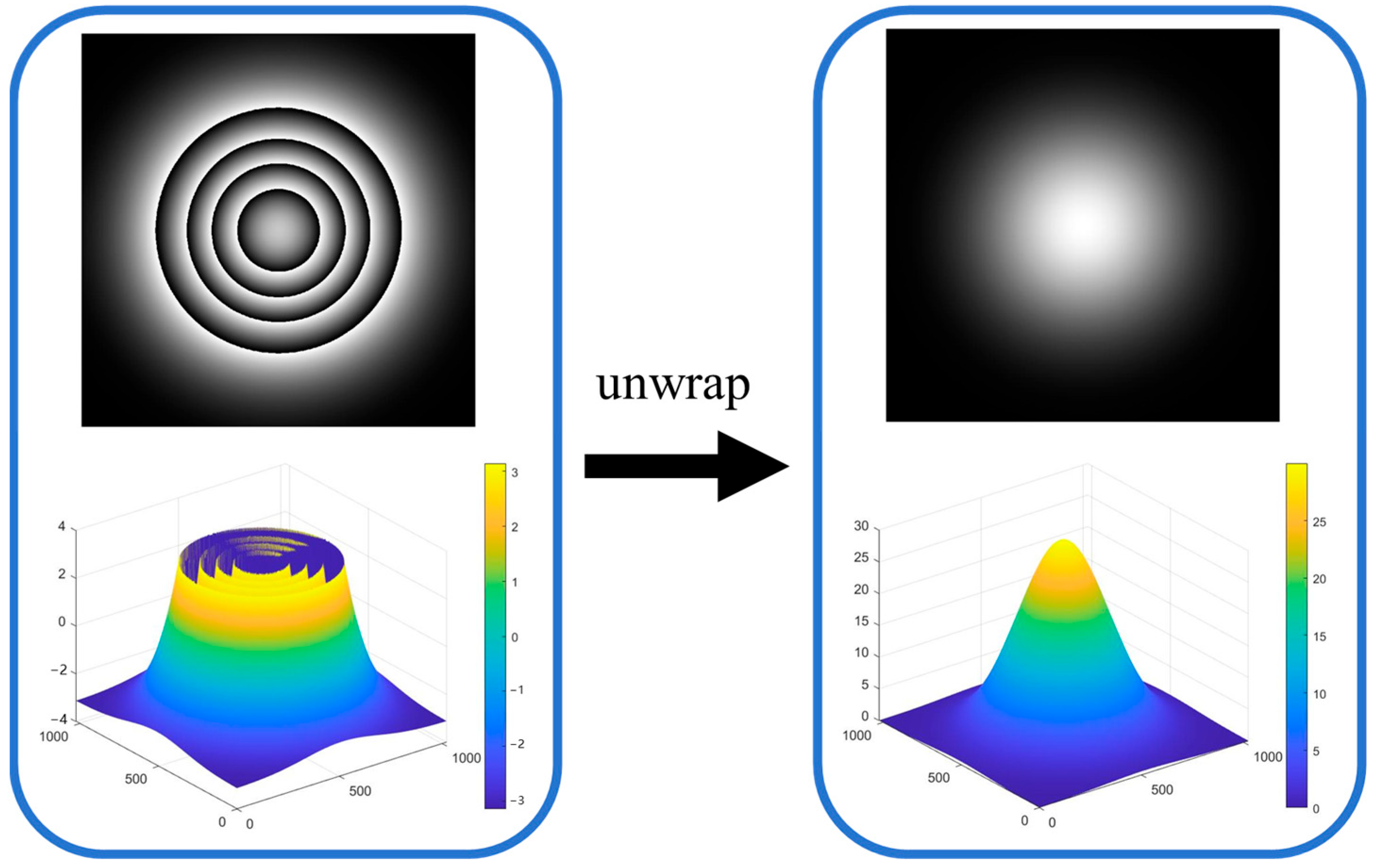
2.2. Phase Unwrapping

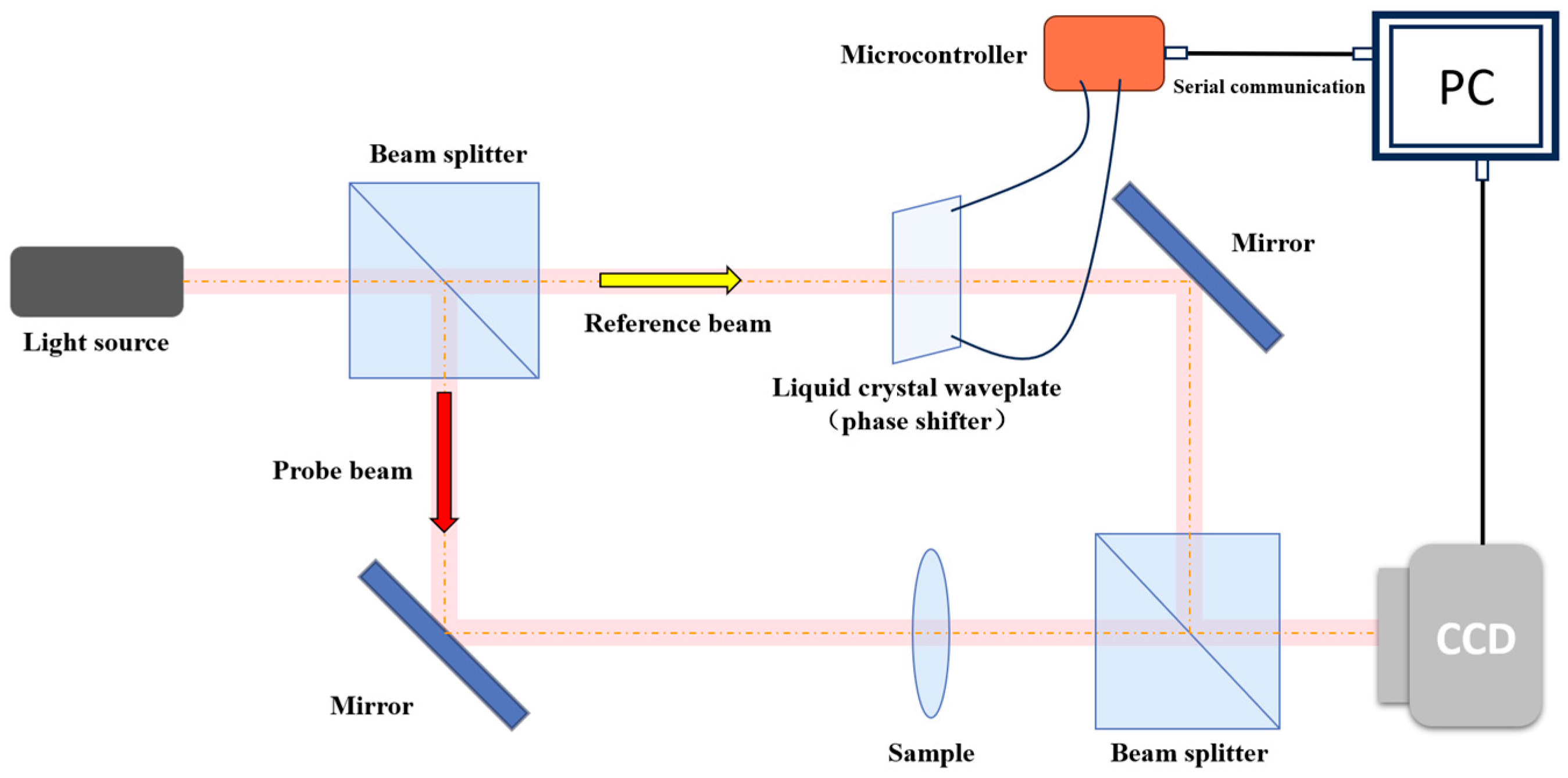
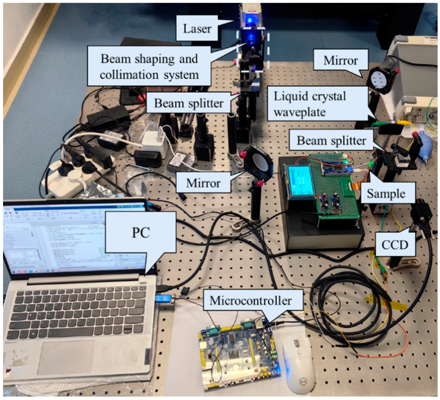
In the phase-shifting algorithm described, the computed phase distribution is constrained by the range of the arctangent function. When phase values approach the boundaries of this range, abrupt jumps occur, resulting in discontinuities that form a wrapped phase. Wrapped phase values are confined to the interval [−π, π].

However, the true phase distribution of the optical wavefront should exhibit continuous variation. To recover this continuous true phase distribution of the object under test, phase unwrapping must be performed on the wrapped phase, e.g., as obtained via the four-step phase-shifting method.

As illustrated in Figure 1, which demonstrates the effect of phase unwrapping applied to a simulated phase distribution—effectively breaking the [−π, π] limitation of the wrapped phase—the processed phase map exhibits continuous variations across an extended, unrestricted range.

The following section briefly introduces the phase-unwrapping algorithm. The phase obtained directly from computation is the wrapped phase. The relationship between the wrapped phase and the true phase is given by

$$\begin{array}{ccc}{\psi }_{ij}=W\left({\varphi }_{ij}\right)={\varphi }_{ij}+2\pi k_{ij}& i=0,1,2,\dots ,M-1;& j=0,1,2,\dots ,N-1\end{array}$$

(5)

In Equation (5), ${\varphi }_{ij}$ represents the continuous true phase distribution, ${\psi }_{ij}$ denotes the wrapped phase, W( ) is the wrapping operator, $k_{ij}$ is an integer, i and j are the pixel coordinates in the x and y directions of the phase image, and M and N are the number of pixels in the x and y directions, respectively. Phase unwrapping aims at estimating the true phase ${\varphi }_{ij}$ from the wrapped phase ${\psi }_{ij}$. This process typically utilizes phase gradients. Since the absolute value of the phase gradient between any two pixels in the true phase should be less than π, those gradients derived from the wrapped phase with absolute values exceeding π require correction. The wrapped phase gradients are defined as [17]

$$\begin{array}{l}{\Delta }_{ij}^x=W\left({\psi }_{\left(i+1\right)j}-{\psi }_{ij}\right)\left(i=0,1,\dots ,M-2;j=0,1,\dots ,N-1\right)\\ {\Delta }_{ij}^x=0\left(i=M-1;j=0,1,\dots ,N-1\right)\\ {\Delta }_{ij}^y=W\left({\psi }_{i\left(j+1\right)}-{\psi }_{ij}\right)\left(i=0,1,\dots ,M-1;j=0,1,\dots ,N-2\right)\\ {\Delta }_{ij}^y=0\left(i=0,1,\dots ,M-1;j=N-1\right)\end{array}$$

(6)

In Equation (6), ${\Delta }_{ij}^x$ and ${\Delta }_{ij}^y$ are the wrapped phase gradients in the x and y directions, respectively. The algorithm employed in this work approximates the true phase gradients using these wrapped phase gradients.

This study utilizes a phase-unwrapping algorithm based on least squares, iteration, and phase gradient correction [17] (Calibrated Phase Unwrapping based on Least-Squares and Iteration, CPULSI). The wrapped phase gradients are corrected using [18]

$$\begin{array}{l}{\Delta }_{ij}^x=\mathrm{sgn}\left({\Delta }_{ij}^x\right)\left|G_x\right|\left|{\Delta }_{ij}^x\right|\ge T_x\\ {\Delta }_{ij}^x={\Delta }_{ij}^x\left|{\Delta }_{ij}^x\right|<T_x\\ {\Delta }_{ij}^y=\mathrm{sgn}\left({\Delta }_{ij}^y\right)\left|G_y\right|\left|{\Delta }_{ij}^y\right|\ge T_y\\ {\Delta }_{ij}^y={\Delta }_{ij}^y\left|{\Delta }_{ij}^y\right|<T_y\end{array}$$

(7)

In Equation (7), sgn( ) denotes the sign function, $T_x$ and $T_y$, $G_x$ and $G_y$ represent thresholds and corrected phase gradients, respectively. They are defined by

$$\begin{array}{l}{T}_x=\sqrt{\mathrm{E}\left[{\left({\Delta }_{ij}^x\right)}^2\right]-{\left[\mathrm{E}\left({\Delta }_{ij}^x\right)\right]}^2}\\ T_y=\sqrt{\mathrm{E}\left[{\left({\Delta }_{ij}^y\right)}^2\right]-{\left[\mathrm{E}\left({\Delta }_{ij}^y\right)\right]}^2}\end{array}$$

(8)

$$\begin{array}{l}{G}_x={\displaystyle \frac{1}{MN}}{\displaystyle \sum _{i=0}^{i=M-1}{\displaystyle \sum _{j=0}^{j=N-1}{\Delta }_{ij}^x}}\\ G_y={\displaystyle \frac{1}{MN}}{\displaystyle \sum _{i=0}^{i=M-1}{\displaystyle \sum _{j=0}^{j=N-1}{\Delta }_{ij}^y}}\end{array}$$

(9)

In Equation (8), E( ) represents the statistical mean value.

Equations (8) and (9) show that $T_x$ and $T_y$ denote the standard deviations of the wrapped phase gradients, while $G_x$ and $G_y$ represent their mean values. This algorithm corrects wrapped phase gradients whose absolute values exceed one standard deviation using the mean values. Subsequently, a least-squares iteration algorithm performs the phase unwrapping. This approach is particularly effective for unwrapping phase maps with high noise levels [17].

3. Experiment Setup

3.1. Measurement System

A phase-shifting interferometer based on a Mach–Zehnder configuration was constructed for acquiring interference patterns. Schematics and photographs of the optical setup are presented in Figure 2 and Figure 3, respectively.

The coherent Gaussian beam (TEM₀₀ mode with M² < 1.2) from the laser source (single longitudinal mode, wavelength: 457 nm, model: MSL-U-457) is split into a reference beam and a test beam by a first beam splitter. The reference beam passes through an electrically controlled liquid-crystal phase shifter, while the test beam passes through the object under test and modulates the phase distribution. The reference beam and the test beam are re-encountered by a second beam splitter and interfere, and the resulting interference pattern is captured by the CCD detection system, which records the intensity distribution.

The constructed phase-shifting interferometer system, shown in Figure 3, utilizes a 457 nm wavelength solid-state laser source (M² < 1.2). The beam is collimated using a beam expander before entering the interferometric system, which comprises two planar mirrors, two beam splitters, a liquid-crystal phase shifter, and the test lens. The imaging system employs a CCD camera with a resolution of 1280 × 1024 pixels and a pixel size of 4.8 μm × 4.8 μm.

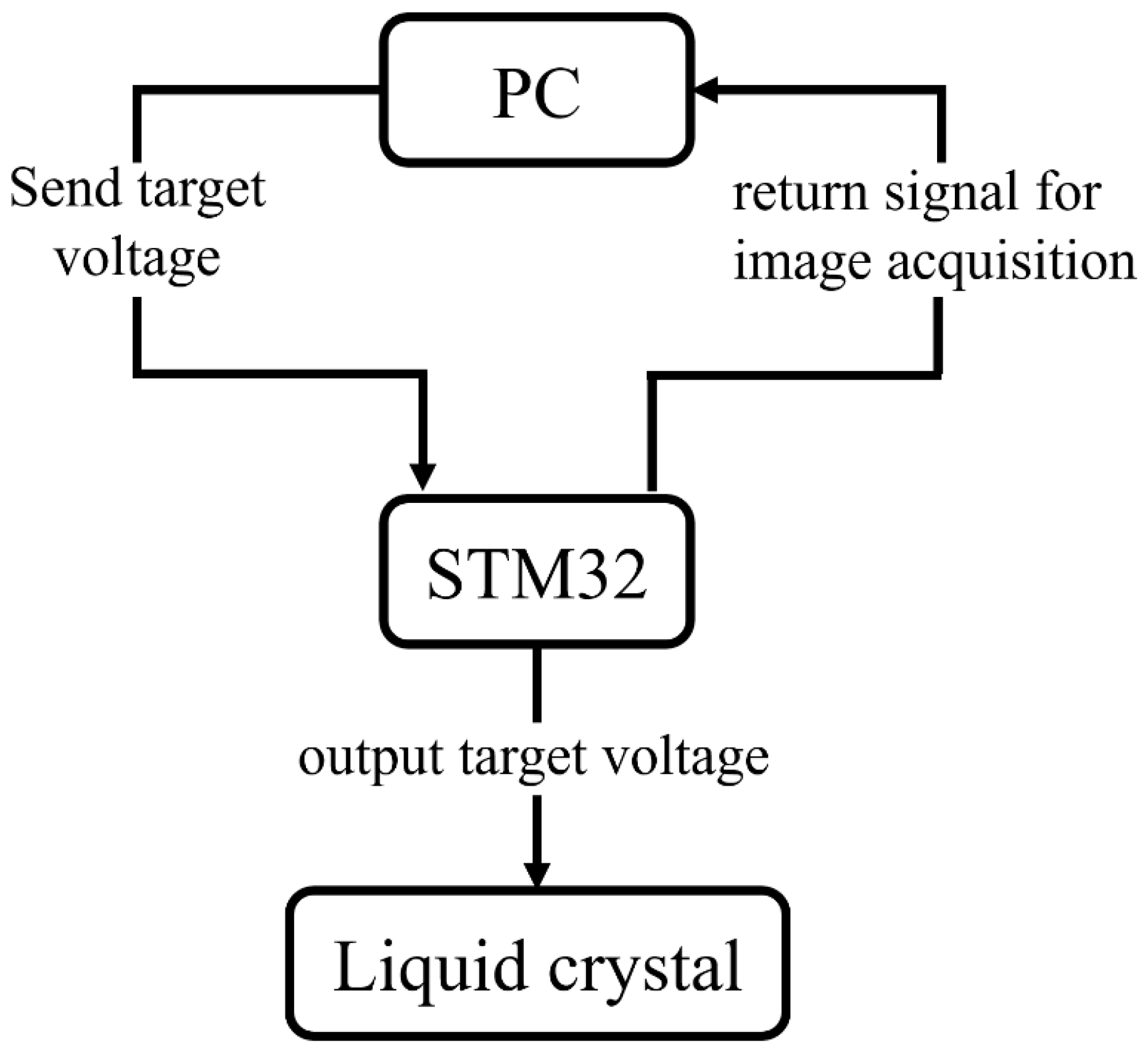
3.2. Automated Image Acquisition System

The automated acquisition system utilizes an STM32F407 microcontroller, which were purchased from JLC corporation, Shenzhen, China. This microcontroller outputs a square-wave AC signal at a specific frequency to drive the LCD phase shifter and establishes serial communication with the PC, enabling efficient automated image acquisition. The image acquisition sequence is shown in Figure 4.

The image acquisition sequence is as follows (Figure 4): The PC transmits a target voltage command to the STM32 microcontroller. Upon receiving the command, the microcontroller calculates the required timing delay and outputs dual-channel square-wave signals with the precise fixed delay. These signals drive the two electrodes of the liquid-crystal cell to generate the target voltage across the cell. Once the voltage application is complete (in some microseconds), the STM32 sends an acquisition trigger signal back to the PC. The PC, upon receiving this trigger, initiates the image capture process (which typically takes 80 ms).

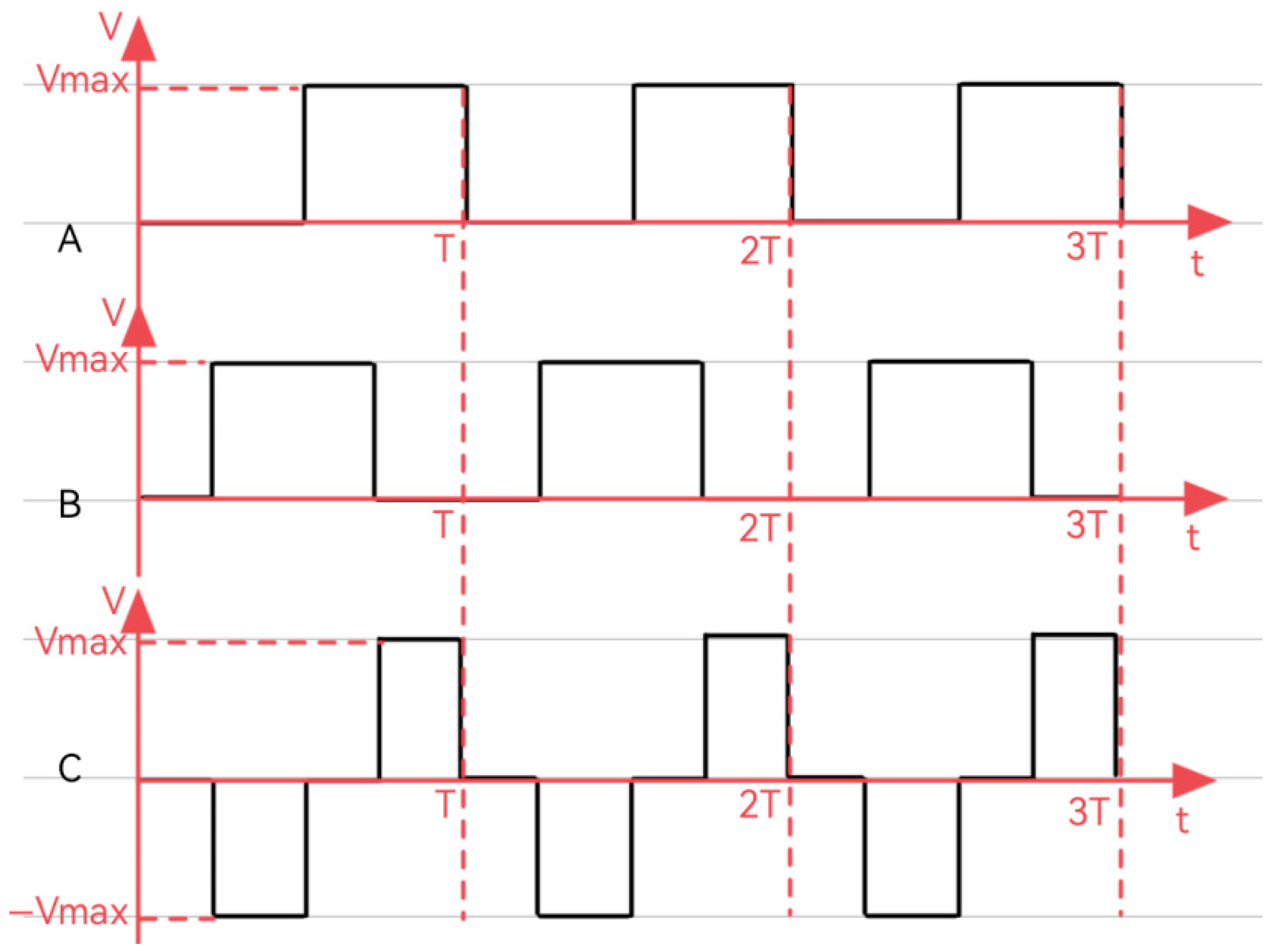
3.2.1. Square-Wave Generation

The system requires the STM32 microcontroller to output two 1 kHz square-wave signals (period: T = 1 ms) via its Digital-to-Analog Converter (DAC) to maximize accuracy and minimize delay. The DAC channels PA4 and PA5 are utilized for this output.

Two timers control the square-wave frequency and delay. Timer TIM2 generates the fundamental frequency, while timer TIM3 controls the duty cycle. The output period is precisely set by configuring the TIM2 prescaler and auto-reload register. TIM3 introduces an adjustable delay between the high and low levels, enabling flexible duty cycle control. The relationship between the target voltage and the duty cycle is

$$V_{\mathrm{rms}}=\sqrt{{\displaystyle \frac{1}{T}}{\displaystyle {\int }_0^T\upsilon {(t)}^2}dt}=\sqrt{{\displaystyle \frac{V_{\max }^{2}DT}{T}}}=V_{\max }\sqrt{DC}$$

(10)

Among them, $V_{\mathrm{rms}}$ is the target voltage, $V_{\max }$ is the amplitude of the square wave, T is the period of AC voltage, and DC is the duty cycle.

As shown in Figure 5, the DAC outputs two square-wave signals (A and B) with the same amplitude $V_{\max }$, frequency 1 kHz, and thus period 1 ms.

The variable time delay between them is τ (0–999 μs). When applied to the two electrodes of the liquid-crystal cell, these signals generate the alternating voltage signal C, whose value is equal to A − B. The high-level duration of each square wave is τ. Thus, the duty cycle DC (duration time of values $+V_{\max }$ and $-V_{\max }$ with respect to the time at 0 V) is the ratio of the delay time τ to the half-period (500 μs):

$$V_{\mathrm{rms}}=V_{\max }\sqrt{{\displaystyle \frac{\tau }{500}}}$$

(11)

Using Equation (11), the required delay τ between the square waves can be calculated. The DAC output voltage is then switched in real time via timer interrupt service routines (ISRs) to generate the target AC signal. Note: the DAC’s maximum output amplitude $V_{\max }$ is typically 3.3 V, requiring appropriate scaling of the desired voltage range, depending on the voltages required to phase-shift the liquid-crystal cell.

3.2.2. Communication Interface

Connection Method: The system employs a USB-to-TTL converter (CH340 module) to establish communication between the STM32F407 microcontroller and the PC. The microcontroller utilizes its USART1 serial port, specifically pins PA9 (TXD, data transmission) and PA10 (RXD, data reception). The PC connection is via USB.

Communication Protocol: Data transmission adheres to a defined frame structure: Frame Header + Frame Content + Frame Trailer. The Frame Header consists of hexadecimal identifier bytes. The Frame Content contains the payload data in string format. The Frame Trailer uses the bytes 0 × 0 D 0 × 0 A (carriage return, line feed) to denote the end of a frame within the interrupt handler. Received data matching the header identifier triggers parsing and subsequent processing.

Function Realization: To mitigate the effects of liquid-crystal response delay (taking approximately 50 ms) and microcontroller output latency on image acquisition (taking approximately 80 ms), the PC-side image capture interval is set to 200 ms per frame. This configuration ensures high precision and low latency while enabling the experimental apparatus to complete the acquisition cycle of four automated images within 1 s.

3.3. Fabrication and Control Method of the Liquid-Crystal Tunable Waveplate

The fabrication of a liquid-crystal (LC) electrically tunable waveplate proceeds through the following principal steps. First, two indium-tin-oxide (ITO)-coated glass substrates are ultrasonically cleaned and subjected to surface treatment. A polyimide (PI) film is then spin-coated onto each electrode layer to serve as the alignment layer; after high-temperature curing, the PI surfaces are mechanically rubbed to impose a well-defined initial orientation on the LC molecules. Next, 5 µm diameter spacer microbeads are uniformly dispensed to define the cell gap, after which a precision adhesive dispenser deposits sealant along the periphery of one substrate. The two ITO glasses are accurately aligned and laminated to form an LC cell, followed by the UV-initiated curing of the sealant. Finally, under vacuum, the nematic LC mixture BHR is introduced into the cell, which is subsequently hermetically sealed.

Upon completion of the cell, conductive silver epoxy is used to bond one end of two copper wires to the ITO electrodes on the respective glass plates, providing external electrical access. The wires are connected to the positive and negative outputs of a 12-bit digital-to-analog converter (DAC) driven by an STM32 microcontroller. To satisfy the drive requirements of the nematic LC material, the DAC is programmed to deliver a 1 kHz square-wave AC signal whose root-mean-square (RMS) amplitude is selected according to the experimentally determined voltage–phase retardation curve of the cell. Because the phase-shifting interferometer operates with a four-step algorithm, four distinct phase retardations are required; consequently, the LC waveplate must be sequentially driven by four discrete RMS voltages delivered in a prescribed timing sequence.

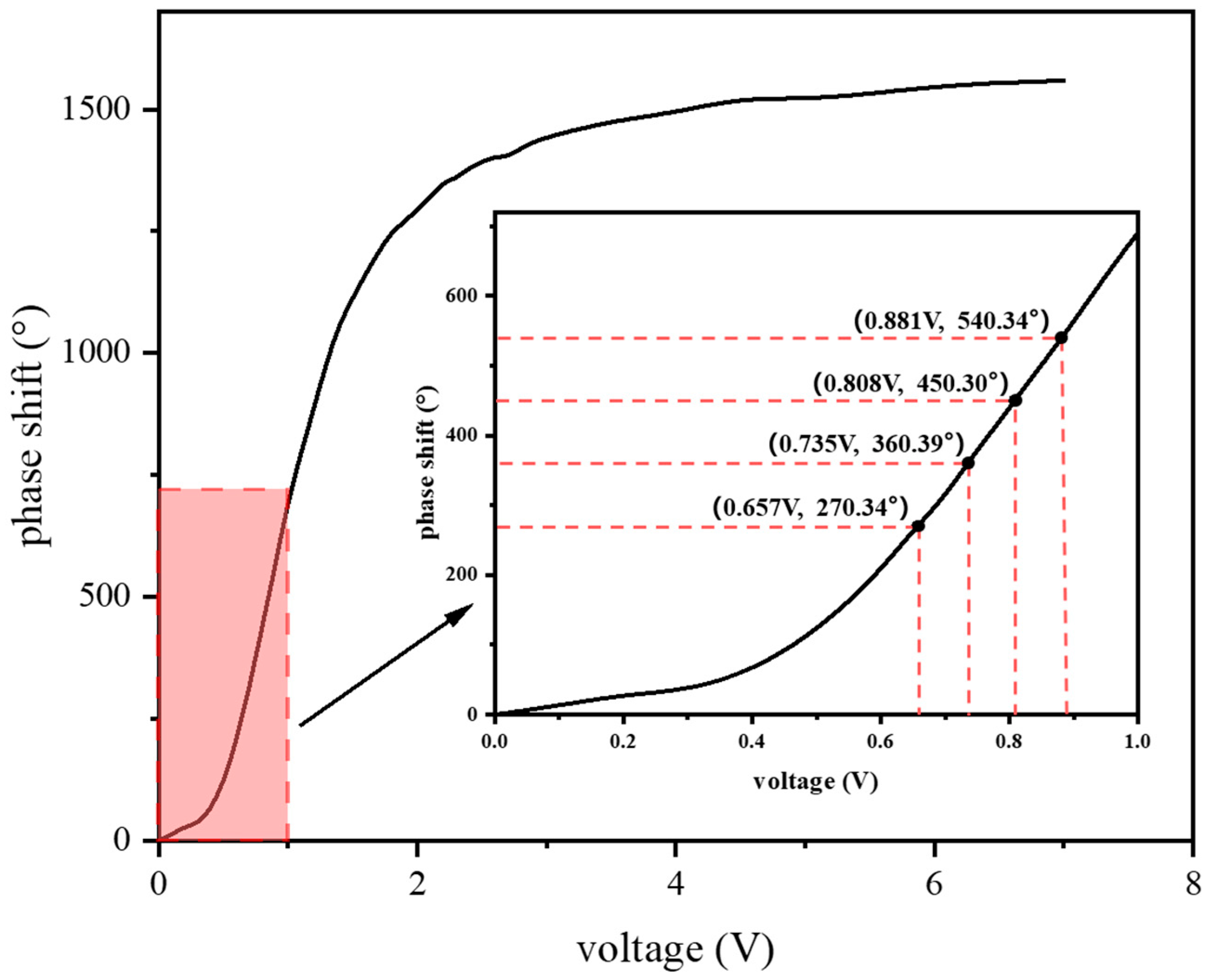
3.4. Characterization of Custom Liquid-Crystal Phase Shifter

The voltage–phase delay relationship was calibrated using the quarter-wave plate compensation method [19], which has been successfully applied in similar studies [20]. The measurement principle is illustrated in Figure 6.

The optical setup comprises input polarizer P₁, the test waveplate (liquid-crystal cell), a quarter-wave plate (QWP), and analyzer P₂ [21]. The transmission axis of P₁ is oriented at 45° to the x-axis, while the transmission axis of P₂ is at 135° (orthogonal to P₁). The test waveplate is positioned after P₁ with its fast and slow axes aligned parallel to the x- and y-axes, respectively. The QWP follows the test waveplate, with its optic axis aligned parallel to transmission axis of P₁.

Using this method, we calibrated the voltage-dependent phase delay of the liquid-crystal waveplate, yielding the relationship shown in Figure 7.

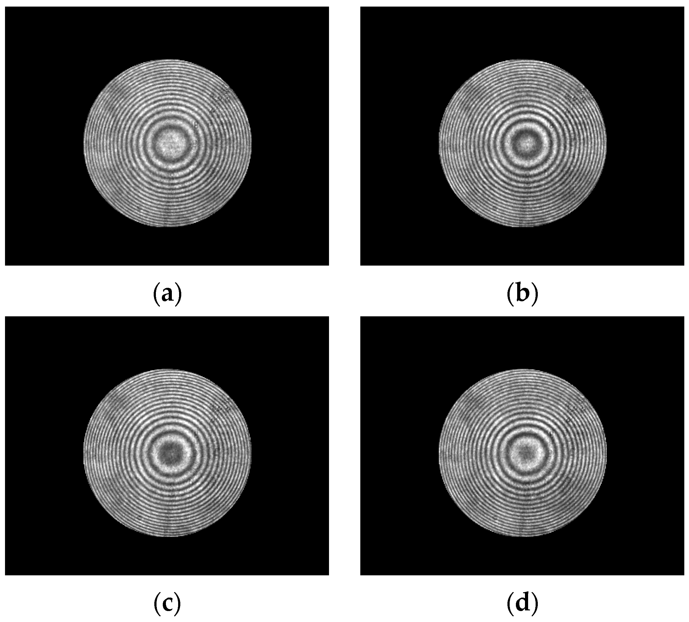
3.5. Interference Pattern Acquisition

Interference patterns are acquired using the CCD camera. The four-step phase-shifting method requires the acquisition of four interference images per measurement cycle, with successive frames separated by 90° phase retardation. Based on the voltage–phase delay characteristic curve of the liquid-crystal waveplate (Figure 7), four voltages corresponding to 90° phase steps within the linear response region were selected: 0.657 V, 0.735 V, 0.808 V, and 0.881 V.

The CCD interfaces with a PC for computer-controlled acquisition. The microcontroller sequentially applies these predetermined voltages to the liquid-crystal phase shifter, signaling the CCD to capture images at each phase setting. This enables the acquisition of four phase-stepped interference images required for wavefront phase calculation.

During acquisition, experimental stability is maintained by optimizing CCD parameters (exposure time, gain) to avoid saturation and ensure image fidelity.

4. Experimental Results

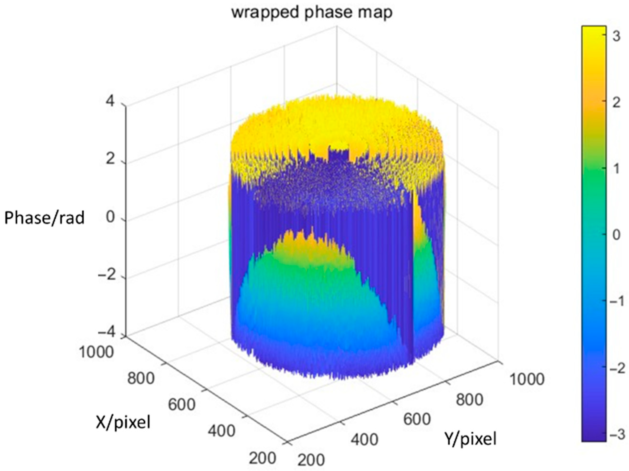
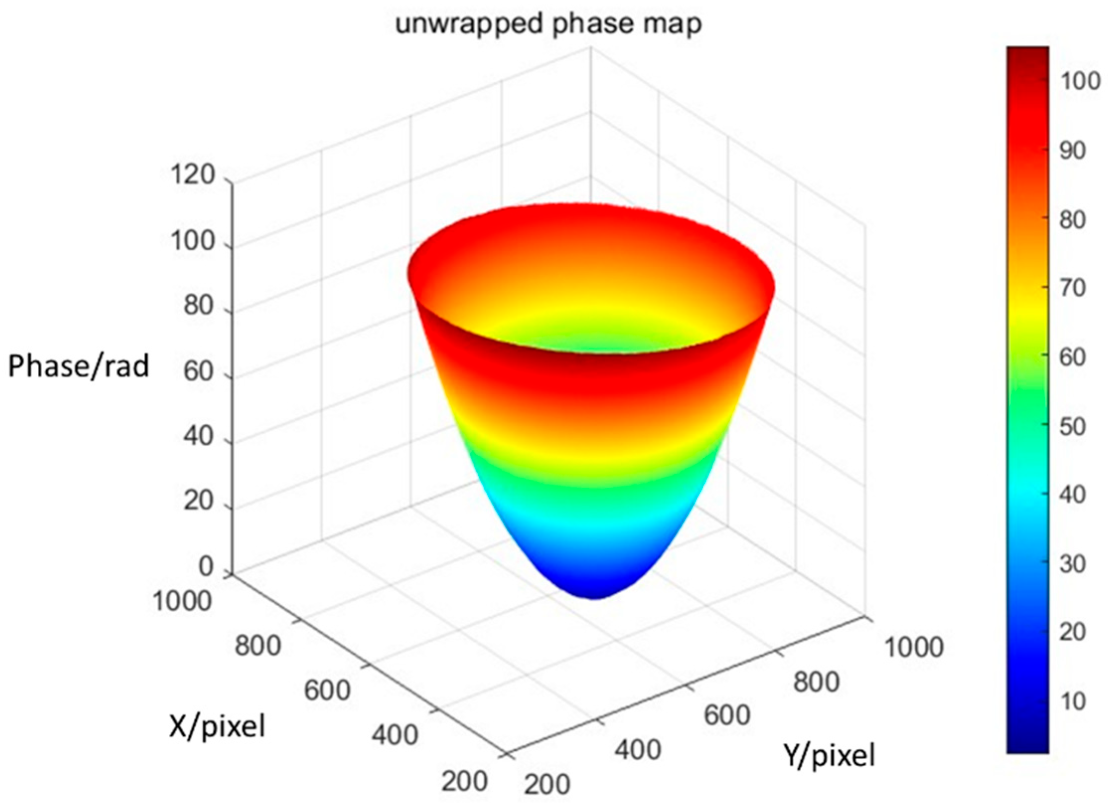
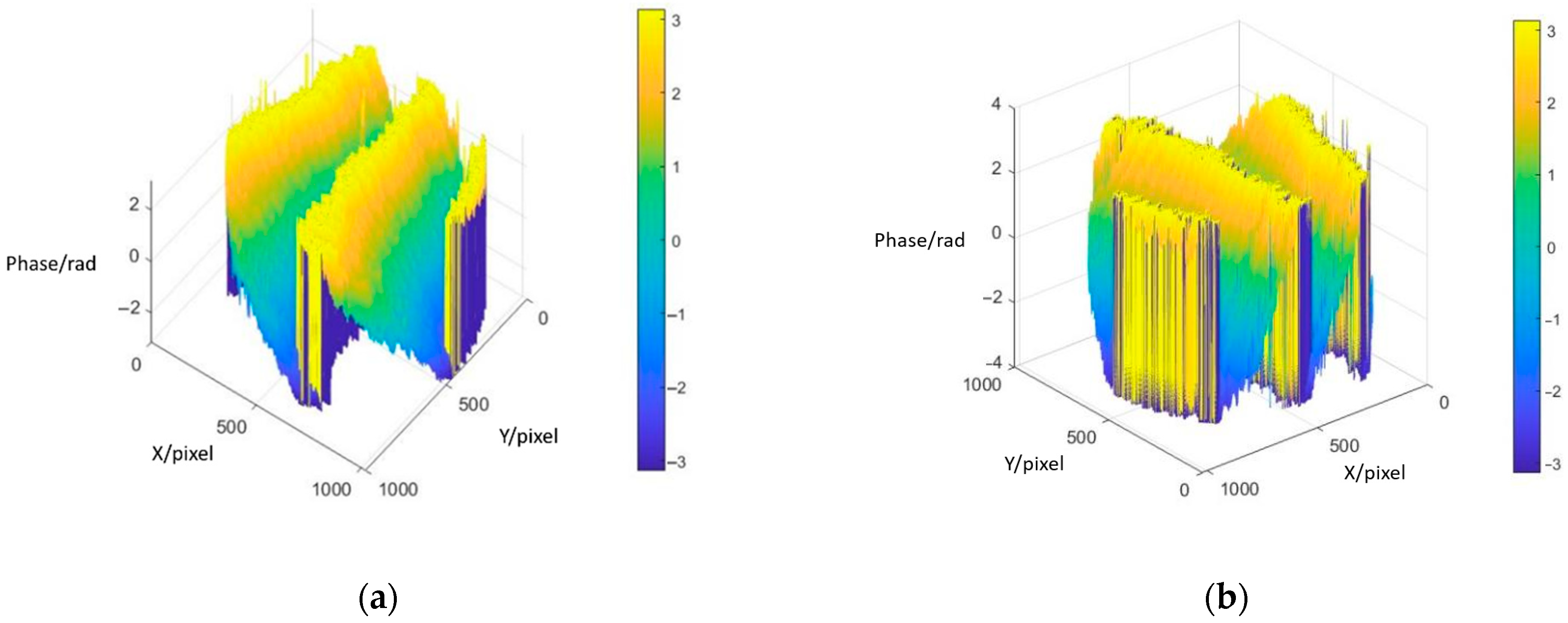
4.1. Phase-Distribution Reconstruction of Test Lens

The experimental setup achieves phase shifting by modulating the voltage (its rms value) across the electrodes of the liquid-crystal phase shifter. At each phase-shift state, interference patterns are captured using a CCD. Four acquired phase-stepped interference images for a plano-convex test lens with a 100 mm focal length are presented in Figure 8.

Applying the four-step phase-shifting algorithm described in Equation (4) to the images of Figure 8 yields the wrapped phase map shown in Figure 9.

The discontinuous wrapped phase in Figure 9 is processed through the CPULSI algorithm [17] (Calibrated Phase Unwrapping based on Least-Squares and Iteration), generating the continuous unwrapped phase distribution of Figure 10.

The focal length of the lens is derived from its phase distribution, accompanied by surface root-mean-square (RMS) error quantification.

The phase-to-optical path difference (OPD) conversion is as follows:

$$OPD={\displaystyle \frac{\phi }{2\pi }}·\lambda$$

(12)

In Equation (12), OPD represents the optical path difference, $\phi$ denotes the phase, and $\lambda$ represents the wavelength of light in a vacuum.

The optical path difference (OPD) of the lens can be fitted to a surface by the following equation:

$$OPD=a\left(x^2+y^2\right)+bxy+cx+dy+e$$

(13)

In general, the optical path difference (OPD) of a spherical wave surface is expressed as [22,23]

$$OPD={\displaystyle \frac{x^2+y^2}{2R_{\omega }}}$$

(14)

where $R_{\omega }$ is the wavefront curvature radius, characterizing the degree of wavefront bending. It can be obtained from Equations (13) and (14) that: $a={\displaystyle \frac{1}{2R_{\omega }}}$. Combined with the geometric optics principle that the focal length f of a thin lens relates to the curvature radius R by $f={\displaystyle \frac{R}{n-1}}$, and the fitting parameter a relates to R by $\left|R\right|={\displaystyle \frac{n-1}{2\left|a\right|}}$ (where n is the refractive index), while considering the relation $R_{\omega }=2f$ between the wavefront curvature radius $R_{\omega }$ and focal length f, the follows that [24]:

$$f={\displaystyle \frac{1}{4a}}$$

(15)

For the 100 mm focal length test lens, fitting yields the following:

$$z=2.5064\left(x^2+y^2\right)+0.0053xy-0.0055x-0.0054y+5.99\times {10}^{-6}{ \mathrm{mm}}^2$$

(16)

The calculated focal length is 99.7 mm (0.26% deviation from the nominal value). The surface RMS error is 9.60 × 10⁻⁹ m (0.021λ at λ = 457 nm), which is comparable to the results obtained using other low-cost phase-shifting techniques [25].

Due to the influence of temperature and voltage fluctuations on the liquid-crystal phase shifter, the stability and repeatability of the measured phase are not very good. In addition, for other two sets of measured data, the focal lengths are 100.9 mm and 108.6 mm, with surface RMS errors of 0.025λ and 0.035λ, respectively.

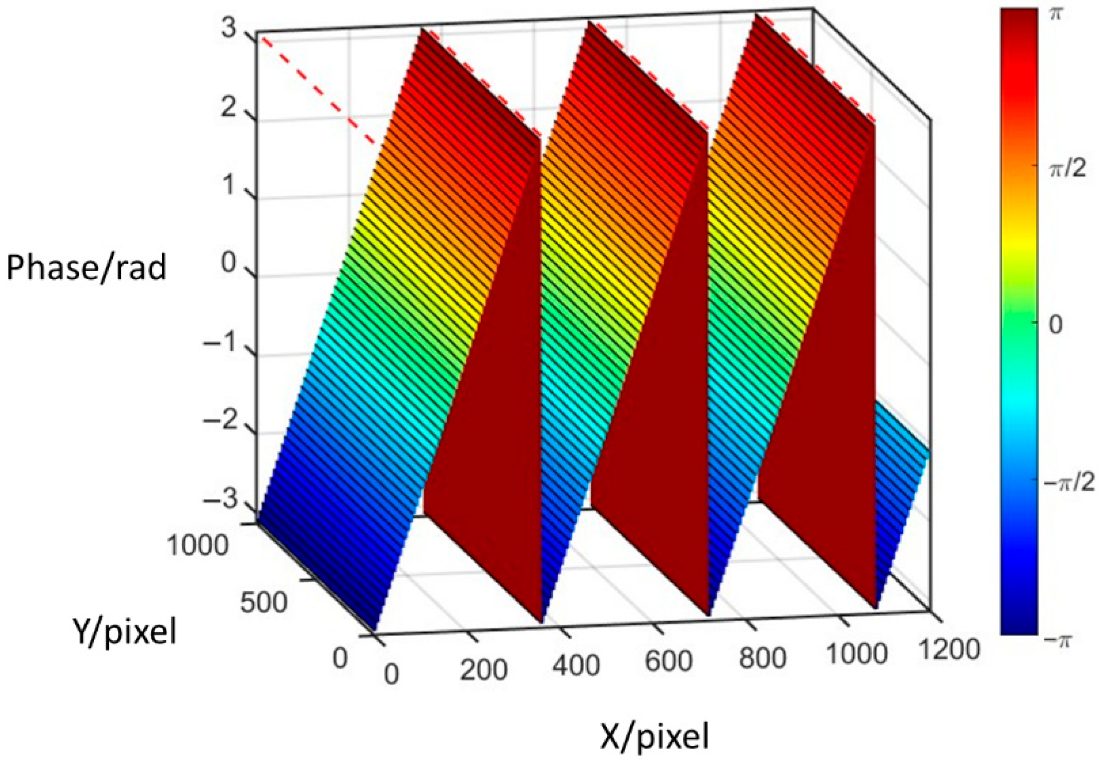
4.2. Phase Characterization of Custom Liquid-Crystal Grating

We further employed the proposed phase-shifting interferometer to evaluate a custom liquid-crystal grating. The experimental results are presented in Figure 11 and Figure 12, and the ideal expected phase profile is shown in Figure 13. The measured phase exhibits a periodic ramp distribution that closely matches the anticipated phase profile of the liquid-crystal grating [25], thereby confirming the validity of the measurement system.

The experimental results reveal a measurable residual error. A preliminary analysis attributes this to three dominant sources: (1) thickness non-uniformities of the liquid-crystal phase shifter introduced during fabrication, which manifest as local flatness errors; (2) wavefront aberrations inherent in the nominally collimated laser beam; and (3) additional wavefront distortions arising from surface imperfections and alignment tolerances of the beam-splitter and folding mirrors.

5. Discussion

5.1. Analysis of Driving Voltage and Phase-Shift Resolution in Liquid-Crystal Phase Shifters

The phase-shifting interferometer constructed in this study employs a liquid-crystal tunable waveplate as the phase shifter; consequently, the phase-shifting accuracy of the waveplate directly governs the measurement precision of the interferometer. The voltage–phase curve of the liquid-crystal phase shifter was calibrated with a 405 nm laser diode, whereas the actual phase-shifting interferometer employs a 457 nm laser. Although the phase values were rescaled according to the wavelength–phase relationship, the birefringence of the liquid-crystal material differs slightly between the two wavelengths, introducing an additional systematic error into the voltage–phase curve. Furthermore, intrinsic measurement uncertainties during the calibration process inevitably degrade the accuracy of the applied voltages.

Because the four-step algorithm requires phase retardations that are exact integer multiples of π/2, we propose a closed-loop strategy: an auxiliary detection path that contains calibrated quarter- and half-wave plates is used to discriminate the actual phase shifts. The four driving voltages are then iteratively adjusted until the measured retardations converge to the nominal values, thereby enhancing the precision of each phase step.

The phase-shifting resolution of a liquid-crystal phase shifter is primarily determined by the applied driving voltage.

According to Equation (11), the output $V_{\mathrm{rms}}$ is determined by both $V_{\max }$ and the temporal delay τ. Consequently, the voltage resolution is at least 12 bits. With the delay time offering 500 discrete steps, the effective resolution will add about 9 bits (512 bits). Then a preliminary estimate yields 4096 × 500 = 204,800 distinguishable levels (~21 bits). Nevertheless, the actual resolution is ultimately constrained by instrumentation limitations; further experimental verification will be pursued when conditions permit.

5.2. Cost Analysis

In this paper, a liquid-crystal tunable waveplate is employed to replace the traditional PZT piezoelectric ceramic as the phase shifter, significantly reducing the equipment cost of the phase-shifting interferometer. According to preliminary estimates, the cost of a precision PZT piezoelectric ceramic and its driving controller is approximately RMB 50,000, while the cost of the homemade liquid-crystal phase shifter and its driving circuit is less than RMB 1000. This offers a significant advantage for scenarios with limited funding budgets.

5.3. Application Scope and Improvement Directions

Owing to the significant cost reduction, this device can be widely applied in fields such as the industrial inspection of optical phase modulation components and the experimental teaching of optical measurement in research institutions and universities. Future improvement directions include enhancing the quality of the homemade liquid-crystal phase shifter, implementing closed-loop calibration of liquid-crystal driving voltages, and optimizing the optical path of the phase-shifting interferometer. These efforts aim to further improve measurement accuracy and ultimately develop a low-cost, integrated testing device.

6. Conclusions

This paper describes an automatic phase-shifting interferometer based on a homemade liquid-crystal phase shifter. The instrument employs a laboratory-fabricated liquid-crystal waveplate as the phase-shifting element, replacing the conventional PZT piezoelectric ceramic phase shifter. Its core advantage lies in enabling convenient and cost-effective phase-distribution measurement through a laboratory-fabricated liquid-crystal phase shifter. By eliminating the need for expensive specialized instruments or procurement of costly PZT phase shifters, this approach significantly reduces the threshold conditions for phase-distribution measurement. This not only eliminates the requirement for a half-reflective and half-transmissive beam splitter in the interferometric optical path, simplifying the optical configuration, but also drastically cuts manufacturing costs by leveraging low-cost homemade components.

The driver control circuit for the liquid-crystal phase shifter and the measurement algorithm software program were developed to achieve automatic rapid (1 s) acquisition of four interferograms, phase-distribution calculation, and phase unwrapping (the whole procedure takes about 1.3 s). The validity of this measurement device is verified through calibration testing of a standard positive lens and phase-distribution testing of a liquid-crystal grating, demonstrating its potential as a low-cost solution for phase-distribution measurement of light waves.

In terms of application scope, the proposed system is particularly well-suited for educational laboratories, low-budget research environments, and industrial settings where high-speed measurement is not a critical requirement. It offers a practical alternative to conventional phase-shifting interferometers (PSIs) in scenarios involving static or quasi-static optical components, such as lens surface profiling, the wavefront analysis of optical elements, and the quality inspection of transparent materials.

References

1. Shen, C.Y.; Li, J.; Mengu, D.; Ozcan, A. Multispectral quantitative phase imaging using a diffractive optical network. Adv. Intell. Syst. 2023, 5, 2300300. [Google Scholar] [CrossRef]
2. Goodman, J.W. Introduction to Fourier Optics, 3rd ed.; Roberts and Company Publishers: Greenwood Village, CO, USA, 2005. [Google Scholar]
3. Zhang, Q.; Lu, S.; Li, J.; Li, D.; Lu, X.; Zhong, L.; Tian, J. Phase-shifting interferometry from single frame in-line interferogram using deep learning phase-shifting technology. Opt. Commun. 2021, 498, 127226. [Google Scholar] [CrossRef]
4. Cheng, Y.-Y.; Wyant, J.C. Phase shifter calibration in phase-shifting interferometry. Appl. Opt. 1985, 24, 3049–3052. [Google Scholar] [CrossRef] [PubMed]
5. Kreis, T. Digital Holographic Interferometry. In Digital Holography and Digital Image Processing; Springer: Dordrecht, The Netherlands, 2005. [Google Scholar]
6. Creath, K. Phase-shifting speckle interferometry. Appl. Opt. 1985, 24, 3053–3058. [Google Scholar] [CrossRef] [PubMed]
7. Zhang, Y.; Tian, X.; Liang, R. Accurate and fast two-step phase shifting algorithm based on principle component analysis and Lissajous ellipse fitting with random phase shift and no pre-filtering. Opt. Express 2019, 27, 20047–20063. [Google Scholar] [CrossRef] [PubMed]
8. Machuca-Bautista, Y.B.; Strojnik, M.; Flores, J.L.; Serrano-García, D.I.; García-Torales, G. Michelson interferometer for phase shifting interferometry with a liquid crystal retarder. Results Opt. 2021, 5, 100197. [Google Scholar] [CrossRef]
9. Cai, D.; Xue, L.; Ning, L. Characteristics of phase-only liquid crystal spatial light modulator. Opt.-Electron. Eng. 2007, 34, 19–23. [Google Scholar]
10. Xia, H.; Montresor, S.; Guo, R.; Li, J.; Yan, F.; Cheng, H.; Picart, P. Phase calibration unwrapping algorithm for phase data corrupted by strong decorrelation speckle noise. Opt. Express 2016, 24, 28713–28730. [Google Scholar] [CrossRef] [PubMed]
11. Morris, M.N.; Millerd, J.; Brock, N.; Hayes, J.; Saif, B.; Stahl, H.P. Dynamic phase-shifting electronic speckle pattern interferometer. In Proceedings of the Optical Manufacturing and Testing VI, San Diego, CA, USA, 31 July–4 August 2005; SPIE: Bellingham, WA, USA, 2005; Volume 5869, p. 58690P. [Google Scholar]
12. Bai, F.; Lang, J.; Gao, X.; Zhang, Y.; Cai, J.; Wang, J. Phase shifting approaches and multi-channel interferograms position registration for simultaneous phase-shifting interferometry: A review. Photonics 2023, 10, 946. [Google Scholar] [CrossRef]
13. Millerd, J.; Brock, N.; Hayes, J.; Kimbrough, B.; Novak, M.; North-Morris, M.; Wyant, J.C. Modern Approaches in Phase Measuring Metrology. In Proceedings of the Optical Measurement Systems for Industrial Inspection IV, Optical Sciences Center, University of Arizona, Tucson, AZ, USA, 13–17 June 2005; SPIE: Bellingham, WA, USA, 2005; Volume 5856, pp. 14–22. [Google Scholar]
14. Li, W.-Z.; Zhou, Z.-Y.; Chen, L.; Li, Y.-H.; Guo, G.-C.; Shi, B.-S. Creating multibeam interference from two-beam interference with cascading and recycling harmonics generation. Phys. Rev. Res. 2025, 7, 023208. [Google Scholar] [CrossRef]
15. Flores, J.L.; Ayubi, G.A.; Di Martino, J.M.; Castillo, O.E.; Ferrari, J.A. 3D-shape of objects with straight line-motion by simultaneous projection of color coded patterns. Opt. Commun. 2018, 414, 185–190. [Google Scholar] [CrossRef]
16. Zhu, Y.; Tian, A. Influence of phase-shifting error of phase-shifting interferometry on the phase accuracy recovery. J. Opt. 2024, 53, 363–382. [Google Scholar] [CrossRef]
17. Xia, H.; Montresor, S.; Picart, P.; Guo, R.; Li, J. Comparative analysis for combination of unwrapping and de-noising of phase data with high speckle decorrelation noise. Opt. Lasers Eng. 2018, 107, 71–77. [Google Scholar] [CrossRef]
18. Zuo, C.; Huang, L.; Zhang, M.; Chen, Q.; Asundi, A. Temporal phase unwrapping algorithms for fringe projection profilometry: A comparative review. Opt. Lasers Eng. 2016, 85, 84–103. [Google Scholar] [CrossRef]
19. Ye, Y.D.; Yan, H.; Wang, F.; Li, J.-M. Phase compensation with rotating quarter waveplate in polarizing beam splitting scheme of laser launched and received in common aperture. High Power Laser Part. Beams 2006, 18, 749–752. [Google Scholar]
20. Muravsky, L.; Ostash, O.; Voronyak, T.; Andreiko, I. Two-frame phase-shifting interferometry for retrieval of smooth surface and its displacements. Opt. Laser Eng. 2011, 49, 305–312. [Google Scholar] [CrossRef]
21. Usman, A.; Bhatranand, A.; Jiraraksopakun, Y.; Kaewon, R.; Pawong, C. Real-time double-layer thin film thickness measurements using modified Signac interferometer with polarization phase shifting approach. Photonics 2021, 8, 529. [Google Scholar] [CrossRef]
22. Ciddor, P.E. Refractive index of air: New equations for the visible and near infrared. Appl. Opt. 1996, 35, 1566–1573. [Google Scholar] [CrossRef] [PubMed]
23. Copland, J.; Neal, D.R.; Neal, D.A. Shack-Hartmann Wavefront Sensor Precision and Accuracy. In SPIE 4779, Proceedings of the Advanced Characterization Techniques for Optical, Semiconductor, and Data Storage Components, Seattle, WA, USA, 11 November 2002; SPIE: Bellingham, WA, USA, 2002. [Google Scholar]
24. Hao, Q.; Liu, Y.; Hu, Y.; Tao, X. Measurement techniques for aspheric surface parameters. Light Adv. Manuf. 2023, 4, 27. [Google Scholar] [CrossRef]
25. Zhang, Z.; Dong, F.; Qian, K.; Zhang, Q.; Chu, W.; Zhang, Y.; Man, X.; Wu, X. Real-time phase measurement of optical vortices based on pixelated micropolarizer array. Opt. Express 2015, 23, 20521–20528. [Google Scholar] [CrossRef] [PubMed]
Figure 1. Unwrap-phase operation effect diagram.
Photonics 12 00722 g001
Figure 2. Schematic diagram of Mach–Zehnder phase-shifting interferometer system.
Photonics 12 00722 g002
Figure 3. Photograph of the experimental Mach–Zehnder interferometer setup, showing the arrangement of optical components on the optical table.
Photonics 12 00722 g003
Figure 4. Flowchart of the automated image acquisition process, showing the communication between PC and microcontroller, voltage control, and image capture sequence.
Photonics 12 00722 g004
Figure 5. Schematic diagram of square-wave signals for driving the liquid-crystal phase shifter, showing two 1 kHz square waves with controlled delay and the resulting AC voltage signal.
Photonics 12 00722 g005
Figure 6. Schematic diagram of phase-delay measurement using the quarter-wave plate compensation method, showing the arrangement of polarizers, quarter-wave plate, and the liquid-crystal cell.
Photonics 12 00722 g006
Figure 7. Voltage–phase delay characteristic curve of the liquid-crystal waveplate, showing the relationship between applied voltage and induced phase delay.
Photonics 12 00722 g007
Figure 8. Interference patterns of 100 mm focal length lens under phase shifts: (a) 0°, (b) 90°, (c) 180°, and (d) 270°.
Photonics 12 00722 g008
Figure 9. Wrapped phase map of 100 mm focal length lens, showing phase discontinuities.
Photonics 12 00722 g009
Figure 10. Unwrapped phase distribution of 100 mm focal length lens, showing continuous phase distribution.
Photonics 12 00722 g010
Figure 11. Wrapped phase map of the liquid-crystal grating: (a) perspective one; (b) perspective two.
Photonics 12 00722 g011
Figure 12. One-dimensional plot of the wrapped phase map of the liquid-crystal grating.
Photonics 12 00722 g012
Figure 13. Ideal phase-distribution map of the liquid-crystal grating.
Photonics 12 00722 g013
Disclaimer/Publisher’s Note: The statements, opinions and data contained in all publications are solely those of the individual author(s) and contributor(s) and not of MDPI and/or the editor(s). MDPI and/or the editor(s) disclaim responsibility for any injury to people or property resulting from any ideas, methods, instructions or products referred to in the content.