The Algorithm for Recognizing Superposition of Wave Aberrations from Focal Pattern Based on Partial Sums


Abstract
1. Introduction
2. Materials and Methods
2.1. Wave Aberrations
2.2. Solution Optimization
3. Results
3.1. One Wave Aberration
3.2. Superposition of Wave Aberrations
4. Discussions
- (1)
- Even simplest superpositions are determined up to the sign at the first stage. If the initial superposition contains only even simplest superpositions, then the solution can be found up to the sign. It is worth noting that if the initial superposition contains at least one odd simplest superposition, then the sign of even simplest superpositions can be checked (specified) only when adding the first odd simplest superposition.
- (2)
- With an increase in the aberration level, the size of the formed PSF pattern expands, so the peripheral part of the analyzed pattern may not fall into the recorded/observed area, which will lead to incorrect results. Therefore, one more analyzed integral characteristic, corresponding to the total intensity value, can be used. Taking into account the standard deviation, it will be of decisive importance if such a characteristic does not match in the reference and current images.
- (3)
- It should be noted that at the k-th stage, the simplest aberration corresponding to the minimum value of the functional may be absent from the desired superposition. In this case, more stages will need to be performed for clarification. As the number of simplest superpositions in the initial set increases, the number of false (not included in the initial superposition) aberrations increases.
5. Conclusions
Author Contributions
Funding
Institutional Review Board Statement
Informed Consent Statement
Data Availability Statement
Acknowledgments
Conflicts of Interest
References
- Rodríguez, A.C.; Booth, M.J.; Turcotte, R. Editorial: Adaptive optics for in vivo brain imaging. Front. Neurosci. 2023, 17, 1188614. [Google Scholar] [CrossRef] [PubMed]
- Roddier, F. Adaptive Optics in Astronomy; Cambridge University Press: Cambridge, UK, 1999. [Google Scholar]
- Lukin, V.P. Adaptive optics in the formation of optical beams and images. Phys.-Uspekhi 2014, 57, 556–592. [Google Scholar] [CrossRef]
- Klebanov, I.M.; Karsakov, A.V.; Khonina, S.N.; Davydov, A.N.; Polyakov, K.A. Wavefront aberration compensation of space telescopes with telescope temperature field adjustment. Comput. Opt. 2017, 41, 30–36. [Google Scholar] [CrossRef]
- Rastorguev, A.A.; Kharitonov, S.I.; Kazanskiy, N.L. Modeling of arrangement tolerances for the optical elements in a space-borne Offner imaging hyperspectrometer. Comput. Opt. 2018, 42, 424–431. [Google Scholar] [CrossRef]
- Chen, Z.; Leng, R.; Yan, C.; Fang, C.; Wang, Z. Analysis of telescope wavefront aberration and optical path stability in space gravitational wave detection. Appl. Sci. 2022, 12, 12697. [Google Scholar] [CrossRef]
- Yudaev, A.V.; Shashkova, I.A.; Kiselev, A.V.; Komarova, A.A.; Tavrov, A.V. Wavefront Correction for the Observation of an Exoplanet against the Background of the Diffraction Stellar Vicinity. J. Exp. Theor. Phys. 2023, 136, 109–130. [Google Scholar] [CrossRef]
- Booth, M.J. Adaptive optical microscopy: The ongoing quest for a perfect image. Light. Sci. Appl. 2014, 3, e165. [Google Scholar] [CrossRef]
- Ji, N. Adaptive optical fluorescence microscopy. Nat. Methods 2017, 14, 374–380. [Google Scholar] [CrossRef]
- Thomas, S. A simple turbulence simulator for adaptive optics. Proc. SPIE 2004, 5490, 766–773. [Google Scholar] [CrossRef]
- Nevzorov, A.A.; Stankevich, D.A. A method of wavefront distortion correction for an atmospheric optical link with a small volume of information transmitted through a service channel. Comput. Opt. 2020, 44, 848–851. [Google Scholar] [CrossRef]
- Du, M.; Loetgering, L.; Eikema, K.S.E.; Witte, S. Measuring laser beam quality, wavefronts, and lens aberrations using ptychography. Opt. Express 2020, 28, 5022–5034. [Google Scholar] [CrossRef] [PubMed]
- Artal, P.; Guirao, A.; Berrio, E.; Williams, D.R. Compensation of corneal aberrations by the internal optics in the human eye. J. Vis. 2001, 1, 1–8. [Google Scholar] [CrossRef] [PubMed]
- Prieto, P.M.; Fernández, E.J.; Manzanera, S.; Artal, P. Adaptive optics with a programmable phase modulator: Applications in the human eye. Opt. Express 2004, 12, 4059–4071. [Google Scholar] [CrossRef]
- Khorin, P.A.; Khonina, S.N.; Karsakov, A.V.; Branchevskiy, S.L. Analysis of corneal aberration of the human eye. Comput. Opt. 2016, 40, 810–817. [Google Scholar] [CrossRef]
- Martins, A.C.; Vohnsen, B. Measuring ocular aberrations sequentially using a digital micromirror device. Micromachines 2019, 10, 117. [Google Scholar] [CrossRef]
- Baum, O.I.; Omel’chenko, A.I.; Kasianenko, E.M.; Skidanov, R.V.; Kazanskiy, N.L.; Sobol, E.N.; Bolshunov, A.V.; Avetisov, S.E.; Panchenko, V.Y. Control of laser-beam spatial distribution for correcting the shape and refraction of eye cornea. Quantum Electron. 2020, 50, 87–93. [Google Scholar] [CrossRef]
- Khorin, P.A.; Khonina, S.N. Simulation of the human myopic eye cornea compensation based on the analysis of aberrrometric data. Vision. 2023, 7, 21. [Google Scholar] [CrossRef]
- Khonina, S.N.; Ustinov, A.V.; Pelevina, E.A. Analysis of wave aberration influence on reducing focal spot size in a high-aperture focusing system. J. Opt. 2011, 13, 095702. [Google Scholar] [CrossRef]
- Abramenko, A.A. Extrinsic calibration of stereo camera and three-dimensional laser scanner. Comput. Opt. 2019, 43, 220–230. [Google Scholar] [CrossRef]
- Hampson, K.M.; Turcotte, R.; Miller, D.T.; Kurokawa, K.; Males, J.R.; Ji, N.; Booth, M.J. Adaptive optics for high-resolution imaging. Nat. Rev. Methods Prim. 2021, 1, 1–26. [Google Scholar] [CrossRef]
- Campbell, H.; Greenaway, A. Wavefront Sensing: From Historical Roots to the State-of-the-Art. EAS Publ. Ser. 2006, 22, 165–185. [Google Scholar] [CrossRef]
- Ling, T.; Jiang, J.; Zhang, R.; Yang, Y. Quadriwave lateral shearing interferometric microscopy with wideband sensitivity enhancement for quantitative phase imaging in real time. Sci. Rep. 2017, 7, 9. [Google Scholar] [CrossRef] [PubMed]
- Yang, W.; Wang, J.; Wang, B. A Method Used to Improve the Dynamic Range of Shack–Hartmann Wavefront Sensor in Presence of Large Aberration. Sensors 2022, 22, 7120. [Google Scholar] [CrossRef]
- Born, M.; Wolf, E. Principles of Optics: Electromagnetic Theory of Propagation, Interference and Diffraction of Light, 7th expanded ed.; Cambridge University Press: Cambridge, UK, 1999; ISBN 978-0-521-64222-4. [Google Scholar]
- Mahajan, V.N. Zernike circle polynomials and optical aberration of system with circular pupils. Appl. Optics 1994, 33, 8121–8124. [Google Scholar] [CrossRef]
- Neil, M.A.A.; Booth, M.J.; Wilson, T. New modal wave-front sensor: A theoretical analysis. J. Opt. Soc. Am. A 2000, 17, 1098–1107. [Google Scholar] [CrossRef]
- Khonina, S.N.; Kotlyar, V.V.; Soifer, V.A.; Wang, Y.; Zhao, D.; Akos, G.; Lupkovics, G.; Podmaniczky, A. Decomposition of a coherent light field using a phase Zernike filter. Proc. SPIE 1998, 3575, 550–553. [Google Scholar] [CrossRef]
- Porfirev, A.P.; Khonina, S.N. Experimental investigation of multi-order diffractive optical elements matched with two types of Zernike functions. Proc. SPIE 2016, 9807, 550–553. [Google Scholar] [CrossRef]
- Khonina, S.N.; Karpeev, S.V.; Porfirev, A.P. Wavefront Aberration Sensor Based on a Multichannel Diffractive Optical Element. Sensors 2020, 20, 3850. [Google Scholar] [CrossRef]
- Khorin, P.A.; Volotovskiy, S.G.; Khonina, S.N. Optical detection of values of separate aberrations using a multi-channel filter matched with phase Zernike functions. Comput. Opt. 2021, 45, 525–533. [Google Scholar] [CrossRef]
- Khorin, P.A.; Porfirev, A.P.; Khonina, S.N. Adaptive Detection of Wave Aberrations Based on the Multichannel Filter. Photonics 2022, 9, 204. [Google Scholar] [CrossRef]
- Khorin, P.A.; Dzyuba, A.P.; Khonina, S.N. Optical wavefront aberration: Detection, recognition, and compensation techniques – a comprehensive review. Opt. Laser Technol. 2025, 191, 113342. [Google Scholar] [CrossRef]
- Dong, B.; Booth, M.J. Wavefront control in adaptive microscopy using Shack-Hartmann sensors with arbitrarily shaped pupils. Opt. Express 2018, 26, 1655–1669. [Google Scholar] [CrossRef] [PubMed]
- Fétick, R.J.L.; Fusco, T.; Neichel, B.; Mugnier, L.M.; Beltramo-Martin, O.; Bonnefois, A.; Petit, C.; Milli, J.; Vernet, J.; Oberti, S.; et al. Physics-based model of the adaptive-optics-corrected point spread function. Applications to the SPHERE/ZIMPOL and MUSE instruments. Astron. Astrophys. 2019, 628, A99. [Google Scholar] [CrossRef]
- Liang, W.; Tao, C.; Xudong, L.; Peifeng, W.; Xinyue, L.; Jianlu, J. Performance measurement of adaptive optics system based on Strehl ratio. J. China Univ. Posts Telecommun. 2016, 23, 94–100. [Google Scholar] [CrossRef]
- Khonina, S.N.; Khorin, P.A.; Serafimovich, P.G.; Dzyuba, A.P.; Georgieva, A.O.; Petrov, N.V. Analysis of the wavefront aberrations based on neural networks processing of the interferograms with a conical reference beam. Appl. Phys. B Laser Opt. 2022, 128, 1–16. [Google Scholar] [CrossRef]
- Xie, K.; Liu, W.; Zhou, Q.; Huang, L.; Jiang, Z.; Xi, F.; Xu, X. Adaptive phase correction of dynamic multimode beam based on modal decomposition. Opt. Express 2019, 27, 13793–13802. [Google Scholar] [CrossRef]
- Volostnikov, V.G. Phase problem in optics. J. Sov. Laser Res. 1990, 11, 601–626. [Google Scholar] [CrossRef]
- Vlasov, N.G.; Sazhin, A.V.; Kalenkov, S.G. Solution of phase problem. Laser Phys. 1996, 6, 401. [Google Scholar]
- More, J.J. The Levenberg-Marquardt Algorithm: Implementation and Theory. In Numerical Analysis; Watson, G.A., Ed.; Springer-Verlag: New York, NY, USA, 1978; pp. 105–116. [Google Scholar]
- Volotovskiy, S.G.; Karpeev, S.V.; Khonina, S.N. Algorithm for reconstructing the complex coefficients of the Laguerre–Gauss modes from the intensity distribution for their coherent superposition. Comput. Opt. 2020, 44, 352–362. [Google Scholar] [CrossRef]


| Stage Number, k | Stage Number, k | ||
|---|---|---|---|
| 0 | 1 | 0 | 1 |
| Field intensity | Partial sums | ||
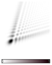
| - | D3,1 = 0.7 D3,–1 = 0.7 | - | D3,1 = 0.7 D3,–1 = 0.7 |
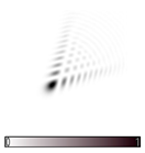 |  |  |  |
| RMS | RMS | ||
| - | 9.9 × 10⁻⁹ | - | 9.9 × 10⁻⁹ |
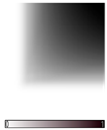
| Recovered phase | Recovered phase | ||
 |  |  |  |
| Stage Number, k | Stage Number, k | ||||
|---|---|---|---|---|---|
| 0 | 1 | 2 | 0 | 1 | 2 |
| Field intensity | Partial sums | ||||
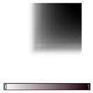
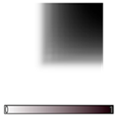
| - | D3,1 = 1.00976 D3,–1 = 1.01018 | D3,1 = 0.7 D3,–1 = 0.7 D2,2 = 2 D2,–2 = 7.9 × 10⁻⁹ | - | D3,1 = 1.00976 D3,–1 = 1.01018 | D3,1 = 0.7 D3,– 1 = 0.7 D2,2 = 2 D2,–2 = 7.9 × 10⁻⁹ |
 |  |  |  |  |  |
| RMS | RMS | ||||
| - | 0.835498 | 9.443586 × 10⁻⁸ | - | 0.077372 | 2.818248 × 10⁻⁹ |
| Recovered phase | Recovered phase | ||||
 |  |  |  |  |  |
| Stage Number, k | ||||
|---|---|---|---|---|
| 0 | 1 | 2 | 3 | 4 |
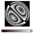
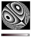
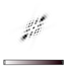
| - | D2.2 = 1.01778 D2,–2 = –1.6780 | D2.2 = 1.57367 D2,– 2 = –1.6213 D3.3 = –0.5814 D3,–3 = –0.5605 | D2,2 = 2.329595 D2,–2 = –0.03393 D3,3 = 0.522402 D3,–3 = –0.56748 D3,1 = 0.319884 D3,–1 = 0.308649 | D2,2 = 1 D2,–2 = –8.8 × 10⁻⁸ D3,3 = 1 D3,–3 = –1 D3.1 = 0.7 D3,–1 = 0.7 D4,4 = –1.4 × 10⁻⁷ D4,–4 = 3.1 × 10⁻⁷ |
| Field intensity | ||||
 |  |  |  |  |
| RMS | ||||
| - | 0.931765 | 1.321484 | 1.009246 | 5.974689 × 10⁻⁷ |
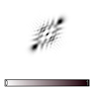
| Partial sums | ||||
 |  |  |  |  |
| RMS | ||||
| - | 0.266242 | 0.348046 | 0.100404 | 3.542697 × 10⁻⁸ |
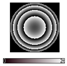
| Recovered phase | ||||
 |  |  |  |  |
| Stage Number, k | |||
|---|---|---|---|
| 0 | 1 | .… | 8 |
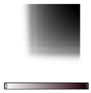
| - | D2,0 = 0.9 D2,2 = 1.08, D2,–2 = 0.78 D3,3 = –2.73, D3,–3 = –2.46 D3,1 = 0.7, D3,–1 = 0.7 D4,4 = 3.84, D4,–4 = 3.84 D4,2 = 0.46, D4,–2 = 0.39 D4,0 = 0.34 | … | … |
| Field intensity | |||
| … | |||
 |  | … |  |
| RMS | |||
| - | 0.833421 | … | 0.338210 |
| Recovered phase | |||
 |  | … |  |
Disclaimer/Publisher’s Note: The statements, opinions and data contained in all publications are solely those of the individual author(s) and contributor(s) and not of MDPI and/or the editor(s). MDPI and/or the editor(s) disclaim responsibility for any injury to people or property resulting from any ideas, methods, instructions or products referred to in the content. |
© 2025 by the authors. Licensee MDPI, Basel, Switzerland. This article is an open access article distributed under the terms and conditions of the Creative Commons Attribution (CC BY) license (https://creativecommons.org/licenses/by/4.0/).
Share and Cite
Volotovsky, S.G.; Khorin, P.A.; Dzyuba, A.P.; Khonina, S.N. The Algorithm for Recognizing Superposition of Wave Aberrations from Focal Pattern Based on Partial Sums. Photonics 2025, 12, 687. https://doi.org/10.3390/photonics12070687
Volotovsky SG, Khorin PA, Dzyuba AP, Khonina SN. The Algorithm for Recognizing Superposition of Wave Aberrations from Focal Pattern Based on Partial Sums. Photonics. 2025; 12(7):687. https://doi.org/10.3390/photonics12070687
Chicago/Turabian StyleVolotovsky, Sergey G., Pavel A. Khorin, Aleksey P. Dzyuba, and Svetlana N. Khonina. 2025. "The Algorithm for Recognizing Superposition of Wave Aberrations from Focal Pattern Based on Partial Sums" Photonics 12, no. 7: 687. https://doi.org/10.3390/photonics12070687
APA StyleVolotovsky, S. G., Khorin, P. A., Dzyuba, A. P., & Khonina, S. N. (2025). The Algorithm for Recognizing Superposition of Wave Aberrations from Focal Pattern Based on Partial Sums. Photonics, 12(7), 687. https://doi.org/10.3390/photonics12070687