Non-Hermitian Control of Tri-Photon and Quad-Photon Using Parallel Multi-Dressing Quantization

Abstract

The fifth-order nonlinear polarizability has been extensively studied in the field of quantum communication due to its ease of manipulation. By adjusting the relative size of the Rabi frequency and dephasing rate of the dressing field, natural non-Hermitian exceptional points can be generated, and further evolution can be achieved by varying the types of dressing fields. However, as the demand for information capacity in quantum communication continues to increase, research on the higher-order seventh-order nonlinear polarizability, based on four-photon states, and the number of coherent channels and resonance positions has gradually come to the forefront. This paper focuses on the simultaneous generation of a seventh-order nonlinear polarizability through a spontaneous eight-wave mixing (SEWM) process in an atomic medium involving four photons. Compared to the fifth-order nonlinear polarizability, the seventh-order polarizability shows an exponential increase in coherent channels and resonance positions due to its strong dressing effect. Additionally, the interaction between the four photons is stronger than that between three photons, making it possible for even the difficult-to-dress eigenvalues to be influenced by the dressing field and dephasing rate, resulting in more complex coherent channels. These are manifested as more complex, damped Rabi oscillations, with periods that can be controlled by the dressing field. These findings may contribute to a promising new method for quantum communication.

1. Introduction

The phenomenon of spontaneous multi-wave mixing and high-order nonlinear processes has renewed interest due to their extensive potential applications [1]. Quantum correlations and entanglement among multiple particles are critical to achieving scalable and efficient quantum information processing [2]. Research into spontaneous multi-wave mixing channels, particularly involving multi-photon processes, is advancing in scientific fields such as quantum communication, quantum operation, and quantum image processing [3,4,5]. Various theoretical frameworks have been proposed to elucidate the relationship between nonlinear optical effects and quantum entanglement. Notable examples include spontaneous six-wave mixing of tri-photon governed by fifth-order nonlinear process, as well as in spontaneous eight-wave mixing process [6].

The χ(3) nonlinearity is widely used for generating spontaneous parametric down-conversion (SPDC) processes in crystals [7], whereas entanglement involving more than two subsystems can be realized through the combination of multiple SPDC processes; therefore, multipartite entanglement can be achieved [8,9]. In recent years, it has been widely discussed where hybrid-cascaded nonlinear processes have been utilized to produce tripartite photons [10]. Furthermore, enhancing the number of quantum coherent channels through photon interactions involves the Autler–Townes effect [11], which manifests when the frequency of the oscillating optical field from a laser closely matches the fundamental eigenfrequency characteristic of the atomic transition [12]. This phenomenon shifts the atomic spectrum and splits the spectral lines, known as dressing states, thereby introducing the concepts of dressing effects with associated physical parameters [13].

The Autler–Townes splitting phenomenon has been extensively recognized as a fundamental mechanism underpinning a wide range of quantum optical effects, notably including electromagnetically induced transparency (EIT) [14]. The Exceptional Point (EP) delineates the critical threshold where a simplex state undergoes a transition into multiple distinct dressed states [15]. The manifestation of an exceptional point arises under critical conditions characterized by the contrast between gain, loss, and mutual coupling [16]. The spontaneous symmetry breaking at the exceptional point is observed as the breakdown of time-reversal symmetry (TRS), experimentally evidenced by optical nonreciprocity in EIT and ATS configurations utilizing warm rubidium atoms [17]. Exceptional points arising from non-Hermitian Hamiltonians have recently appeared as innovative methodologies for engineering the response of open physical systems [18]. While the fundamental nature of PT symmetry remains under debate, it exhibits characteristics common to natural symmetries: it can undergo spontaneous symmetry breaking with a transition from real to complex spectra, whereas a phase transition can occur in the system, resulting in the restoration of the symmetry breaking [19]. Non-Hermiticity also provides an approach to phase matching in multi-wave mixing processes [20]. The interplay between gain, loss, and coupling strength across different optical components unveils numerous novel opportunities in photonics for the generation, control, and transmission of light [21].

Because of the nonlinear process, the coherent channels lead to a state of dressing field effect [22]. In this energy level framework, various dressed levels are considered, leading to distinct coherence states, which correspond to the energy level structure [13]. Based on the energy conservation conditions at these resonance positions, the number of coherent channels in the EWM process within the system can be determined [23]. Additionally, interference among the multi-modes of the quad-photons results in the four-photon coincidence count manifesting as a damped Rabi oscillation [24].

In this paper, we develop a theoretical model of non-Hermiticity systems in an atomic energy level system, for simultaneously generating narrow-band tri-photons and quad-photons based on the spontaneous six-wave mixing (SSWM) and the spontaneous eight-wave mixing (SEWM) processes in rubidium atomic vapor. Here, we observe the real and imaginary parts of the nonlinear optical responses with different dressing fields. We provide a comprehensive overview, synthesis, and examination of spontaneous multi-wave mixing phenomena occurring in 85Rb atoms. In addition, we investigate the advantages of the quad-photon system in terms of quantum information capacity during quantum communication by comparing the multi-channel periods of the three-photon and four-photon optical response coherent channels. Based on the relationship between coherent channels and photon numbers, we deduce that the quantum information capacity equals n to the power of m, where n is the number of coherent channels generated by the nonlinear optical response, and m is the number of photons involved in the nonlinear optical response. Furthermore, we discovered interactions between coherent channels of different eigenvalues, an effect that leads to energy level splitting induced by the dressing field even in eigenvalues that are typically unaffected by the dressing field. This finding allows us to manipulate the energy levels of eigenvalues that are less influenced by the dressing field using the relationship between the Rabi oscillation frequency and the decoherence rate. The aforementioned patterns can be reflected in the changes in peak values and peak numbers simulated by the Kappa value, as well as in the variations in the period and decay rate observed in the simulation of coincidence counting rates.

2. Basic Theory and Simulation of Tri-Photons System

2.1. Single-Dressing Effect

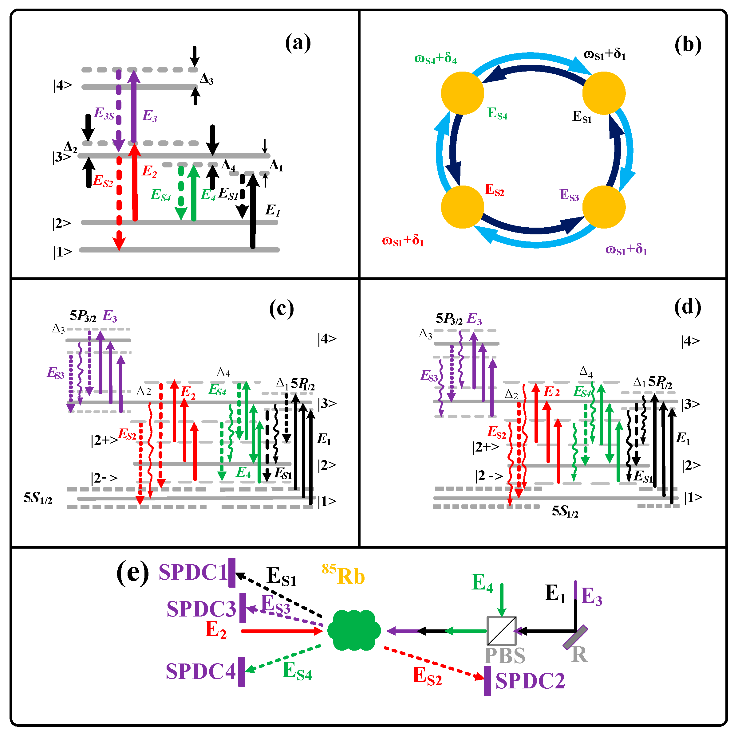
Figure 1a illustrates a streamlined experimental arrangement for the process under investigation, wherein the spontaneous six-wave mixing (SSWM) phenomenon takes place within a hot ⁸⁵Rb atomic vapor. The rubidium vapor is contained inside a slender, elongated cylindrical cell of length. The corresponding atomic energy conservation is shown in Figure 1b. In this setup, the atomic ensemble predominantly occupies the ground state |1>.

A pump beam ${\mathit{E}}_1$ (frequency ${\mathit{\omega }}_1$, wave vector ${\mathit{k}}_1$, Rabi frequency ${\mathrm{G}}_1$, wavelength 780 nm) with detuning ${\mathsf{\Delta }}_1$ is employed to drive the atomic transition |1> to |3>. The detuning ${\mathsf{\Delta }}_{\mathrm{i}(\mathrm{i}=\mathrm{1,2},3)}$ refers to the deviation or difference between the frequency of the driving field (the laser frequency) and the intrinsic resonance frequency of the system resonant transition frequency). The detuning was defined as ${\mathsf{\Delta }}_{\mathrm{i}}={\mathit{\Omega }}_{\mathit{i}}-{\mathit{\omega }}_{\mathit{i}}$, ${\mathit{\Omega }}_{\mathit{i}}$ is the resonant transition frequency, and ${\mathsf{\omega }}_{\mathrm{i}}$ is the laser frequency of ${\mathrm{E}}_{\mathrm{i}}$. ${\mathit{E}}_2$ (${\mathit{\omega }}_2$, ${\mathit{k}}_2$, ${\mathit{G}}_2$, 780 nm, |2> to |4>) with detuning ${\mathsf{\Delta }}_2$ and ${\mathit{E}}_3$ (${\mathit{\omega }}_3$, ${\mathit{k}}_3$, ${\mathit{G}}_3$, 776 nm, |1> to |4>) with detuning ${\mathsf{\Delta }}_3$ are just like ${\mathit{E}}_1$. According to the principle of conservation of momentum, ${\mathrm{k}}_1+{\mathrm{k}}_2+{\mathrm{k}}_3={\mathrm{k}}_{\mathrm{s}1}+{\mathrm{k}}_{\mathrm{s}2}+{\mathrm{k}}_{\mathrm{s}3}$. Regarding the energy level transition process, it can be represented in the form of a perturbation chain as follows:

$${\rho }_{11}^{\left(0\right)}\stackrel{{\omega }_1}{\to }{\rho }_{31}^{\left(1\right)}\stackrel{{\omega }_{S1}}{\to }{\rho }_{21}^{\left(2\right)}\stackrel{{\omega }_2}{\to }{\rho }_{31}^{\left(3\right)}\stackrel{{\omega }_3}{\to }{\rho }_{41}^{\left(4\right)}\stackrel{{\omega }_{s3}}{\to }{\rho }_{31}^{\left(5\right)}$$

The SSWM process satisfied the energy conservation principle ${\mathsf{\omega }}_1+{\mathsf{\omega }}_2+{\mathsf{\omega }}_3={\mathsf{\omega }}_{\mathrm{s}1}+{\mathsf{\delta }}_1+{\mathsf{\omega }}_{\mathrm{s}2}+{\mathsf{\delta }}_2+{\mathsf{\omega }}_{\mathrm{s}3}+{\mathsf{\delta }}_3$. Here, ${\mathsf{\omega }}_{\mathrm{s}\mathrm{i}}$ ($\mathrm{i}$ = 1, 2, 3) denotes the frequency of the emitted photons. In the process illustrated in Figure 1a, using single dressing as an example, Figure 1c shows that a single channel emerges when the dressing Rabi frequency is dominant (represented by a dashed line), while two channels arise when the imaginary component dominates (represented by a wavy line). Thus, depending on the varying intensities of the dressing field and the dephasing rate, the number of coherent channels in the real and imaginary components manifests on either side of the exceptional point (EP). The solid lines in Figure 1c,d indicate the pumping lasers, the dash line indicates the dressing Rabi frequency-induced photon channel, and the wavy line represents the dephasing rate-induced photon channel. Figure 1c represents the coherent channels mainly induced by the strong dressing Rabi frequency Gi. The energy level splitting occurring under the strong dressing condition of Gi > Γij is denoted as the in-phase constructive dressing effect. The dash lines correspond to two splitting coherent channels induced by dressing Rabi frequency and the wavy line in the middle represents the decay in multi-photon coincidence counts resulting from the imaginary part of the eigenvalue. The diagrams in Figure 1d exhibit the energy level splitting generated under the dominating dephasing rate with weak-dressing Rabi frequency, which is considered as the out-of-phase destructive dressing effect. And two splitting coherent channels can also be produced under the weak dressing condition of Gi < Γij. For this region, the coherent channels induced by dephasing rates are symbolized by the wavy lines while the dash line represents the decay produced by the real part of eigenvalue. As for the case of Gi = Γij, without further energy level splitting, only one unsplit photon channel can be produced. And the energy level distribution would exhibit high similarity to the initial configuration of the bare atom presented in Figure 1c,d. Such a critical transition point between the strong dressing and weak dressing conditions can be denoted as the exceptional point of the atomic, natural, non-Hermitian system.

The ${\mathsf{\chi }}_{\mathrm{s}\mathrm{i}}$ is to obtain the perturbation chain ${\mathsf{\rho }}_{\mathrm{s}\mathrm{i}}^{\left(5\right)}$.

$${\chi }_{S1}^{\left(5\right)}={\mathrm{G}}_1{\mathsf{\rho }}_{S1}^{\left(5\right)}$$

$${\chi }_{S1}^{\left(5\right)}={\displaystyle \frac{2N{\mu }_{13}{\mu }_{23}^2{\mu }_{34}^2}{{\epsilon }_0{\mathrm{\hslash }}^5}}{\displaystyle \frac{1}{{\mathrm{d}}_1{\mathrm{d}}_2{\mathrm{d}}_3{\mathrm{d}}_4{\mathrm{d}}_5}}$$

(1)

Here, $d_1={\Gamma }_{31}+i{\mathsf{\Delta }}_1$, $d_2={\Gamma }_{21}-i{\delta }_3-i{\delta }_2$, $d_3={\Gamma }_{31}-i{\delta }_3-i{\delta }_2+i{\mathsf{\Delta }}_2$, $d_4={\Gamma }_{41}-i{\delta }_3-i{\delta }_2+i{\mathsf{\Delta }}_2+i{\mathsf{\Delta }}_3$, $d_5={\Gamma }_{31}-i{\delta }_2+i{\mathsf{\Delta }}_2$, when considering the case of the single-dressing effect of ${\mathrm{E}}_2$ only, the formula can be written as follows:

$${\chi }_{S1}^{\left(5\right)}={\displaystyle \frac{2N{\mu }_{13}{\mu }_{23}^2{\mu }_{34}^2}{{\epsilon }_0{\mathrm{\hslash }}^5}}{\displaystyle \frac{1}{{\mathrm{d}}_1{\mathrm{d}}_2{\mathrm{d}}_3{\mathrm{d}}_4{\mathrm{d}}_5^{\prime }}}$$

(2)

$\mathrm{w}\mathrm{h}\mathrm{e}\mathrm{r}\mathrm{e} {\mathrm{d}}_5^{\mathrm{\prime }}={\mathrm{d}}_5+{{\mathrm{G}}_2}^2/({\mathsf{\Gamma }}_{21}-\mathrm{i}{\mathsf{\delta }}_2)$. The expression for ${\mathrm{d}}_5^{\mathrm{\prime }}=0$ can be simplified as follows: $-{\mathsf{\delta }}_2^2+(-\mathrm{i}{\mathsf{\Gamma }}_{21}-\mathrm{i}{\mathsf{\Gamma }}_{31}+{\mathsf{\Delta }}_2){\mathsf{\delta }}_2+{\mathsf{\Gamma }}_{21}{\mathsf{\Gamma }}_{31}+\mathrm{i}{\mathsf{\Gamma }}_{21}{\mathsf{\Delta }}_2+{{\mathrm{G}}_2}^2=0$. By tuning the ratio of the Rabi frequency ${\mathrm{G}}_2$ and the out-of-phase rate ${\Gamma }_{42}$ of the corresponding dressing field, one can effectively manipulate the sign of the resulting expression. The solution is the eigenvalue $\mathsf{\delta }=\mathrm{a}+\mathrm{i}\mathrm{b}$. When obtaining the pure real part without the imaginary part, ignore b² to solve a and ignore the imaginary part to solve the value of b. The solution of $\mathrm{a}$ are ${\mathrm{a}}_{1\pm }=({\mathsf{\Delta }}_2\pm ({\mathsf{\Delta }}_2^2-4(-{\mathsf{\Gamma }}_{21}{\mathsf{\Gamma }}_{31}-{{\mathrm{G}}_2}^2){)}^{1/2})/2$, as well as the corresponding linewidth ${\mathrm{b}}_{1\pm }=-({\mathsf{\Gamma }}_{21}+{\mathsf{\Gamma }}_{41})/2+\left({\mathsf{\Delta }}_3{\mathsf{\Gamma }}_{11}\right)/\left(2{\mathrm{a}}_{1\pm }\right)$. Therefore, the single-dressing effect can generate second-order EP. Similarly, the solution of $\mathrm{b}$ are ${\mathrm{b}}_{2\pm }=-{\mathsf{\Gamma }}_{21}-{\mathsf{\Gamma }}_{31})\pm ((-{\mathsf{\Gamma }}_{21}-{\mathsf{\Gamma }}_{31}{)}^2+4(-{\mathsf{\Gamma }}_{21}{\mathsf{\Gamma }}_{31}-{{\mathrm{G}}_2}^2){)}^{1/2}/2$, as well as the corresponding linewidth ${\mathrm{a}}_{2\pm }={\mathsf{\Delta }}_2/2+\left({\mathsf{\Delta }}_2{\mathsf{\Gamma }}_{21}\right)/\left(2{\mathrm{b}}_{2\pm }\right)$. It can be denoted by the second-order dressing-coupled Hamiltonian matrix (S3) and (S4) in the Supplement material, respectively.

The main parameters are as follows: ${\Gamma }_{21}=0.5,{\Gamma }_{31}=0.4,{\Gamma }_{41}=0.5,{\mathsf{\Delta }}_1{=0.1,\mathsf{\Delta }}_2=0.2,{\mathsf{\Delta }}_3=0.2$.

The photon random coincidence counting rate (Rcc) refers to the rate at which two or more detectors simultaneously register photon detection events within a defined temporal window. This metric is fundamental in quantum optics experiments for characterizing photon correlations, entanglement, and non-classical light properties. By analyzing coincidence counts, one can infer the degree of temporal or spatial correlation between photons, which is crucial for verifying quantum coherence and demonstrating phenomena such as photon bunching or antibunching. The photon coincidence counting rate thus serves as a key observation in the study of quantum states of light and their interactions. Tri-photons can be represented by the tri-photon amplitude $\mathrm{B}({\mathsf{\tau }}_{\mathrm{S}1},{\mathsf{\tau }}_{\mathrm{S}2},{\mathsf{\tau }}_{\mathrm{S}3})$ and the averaged tri-photon coincidence counting rate (Rcc), where $\mathrm{B}({\mathsf{\tau }}_{\mathrm{S}1},{\mathsf{\tau }}_{\mathrm{S}2},{\mathsf{\tau }}_{\mathrm{S}3})$ can be defined as follows:

$$\mathrm{B}\left({\mathsf{\tau }}_1,{\mathsf{\tau }}_2,{\mathsf{\tau }}_3\right)=\mathrm{W}\int \mathrm{d}{\mathsf{\delta }}_1\int \mathrm{d}{\mathsf{\delta }}_2\int \mathrm{d}{\mathsf{\delta }}_3{\mathsf{\chi }}_{\mathrm{S}1}^{\left(5\right)}$$

$${\mathrm{e}}^{-\mathrm{i}{\mathsf{\delta }}_1{\mathsf{\tau }}_{12}}{\mathrm{e}}^{-\mathrm{i}{\mathsf{\delta }}_2{\mathsf{\tau }}_{14}}{\mathrm{e}}^{-\mathrm{i}{\mathsf{\delta }}_3{\mathsf{\tau }}_{23}}$$

(3)

The temporal correlation of the generated photons was examined through Rcc. Rcc is defined as follows:

$$\mathrm{R}\mathrm{c}\mathrm{c}=\underset{\mathrm{T}\to \mathrm{\infty }}{\mathrm{l}\mathrm{i}\mathrm{m}}{\mathrm{T}}^{-1}{\int }_0^{\mathrm{T}}\mathrm{d}{\mathrm{t}}_{\mathrm{s}1}{\int }_0^{\mathrm{T}}\mathrm{d}{\mathrm{t}}_{\mathrm{s}2}{\int }_0^{\mathrm{T}}\mathrm{d}{\mathrm{t}}_{\mathrm{s}3}{\mathrm{G}}^{\left(3\right)}\times$$

$${\mathrm{M}}_1\left({\mathrm{t}}_{\mathrm{s}2}-{\mathrm{t}}_{\mathrm{s}1}\right){\mathrm{M}}_1\left({\mathrm{t}}_{\mathrm{s}3}-{\mathrm{t}}_{\mathrm{s}1}\right)$$

(4)

where ${\mathrm{G}}^{\left(3\right)}$ is the third-order intensity correlation function of the tri-photon, which can be written as follows: ${\mathrm{G}}^{\left(3\right)}=\mathrm{B}({\mathsf{\tau }}_1,{\mathsf{\tau }}_2,{\mathsf{\tau }}_3{)}^2$. Therefore, the temporal correlation characteristics can be studied via optical responses. We use the residue theorem to calculate $\mathrm{R}\mathrm{c}\mathrm{c}$. The specific form is as follows: ${\int }_{\mathrm{l}}\mathrm{f}\left(\mathrm{z}\right)/{(\mathrm{z}-\mathrm{a})}^{\mathrm{n}}\mathrm{d}\mathrm{z}=2\mathrm{i}\mathsf{\pi }/\left(\mathrm{n}-1\right)!{\mathrm{f}}^{(\mathrm{n}-1)}\left(\mathrm{a}\right)$. ${\mathrm{f}}^{(\mathrm{n}-1)}\left(\mathrm{a}\right)$ is the derivative of the function $\mathrm{f}$ at $\mathrm{x}=\mathrm{a}$, reflecting the relationship between the higher-order derivative and the loop integral.

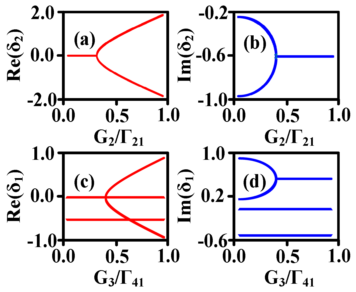
The eigenvalue splits when dressed by laser field ${\mathrm{G}}_2$. The real and imaginary parts have different phase transition points and opposite trends. The calculation result is obtained from dressing-coupled matrix (S1) and Equation (2). When the ratio of the dressing Rabi frequency ${\mathrm{G}}_2$ to the corresponding energy level dephasing rate ${\mathsf{\Gamma }}_{21}$ is considered on the right side of the exceptional point (EP), the root of Equation (2) becomes positive. In this case, the real part exhibits a splitting behavior dominated by ${\mathrm{G}}_2$, which leads to in-phase constructive dressing. Furthermore, a larger value of ${\mathrm{G}}_2/{\mathsf{\Gamma }}_{21}$ enhances the splitting of the real component.

Conversely, on the left side of the EP, when the ratio ${\mathrm{G}}_2/{\mathsf{\Gamma }}_{21}$ is taken into account and the root of Equation (2) is negative, the imaginary part begins to split. This regime is dominated by the dephasing rate ${\mathsf{\Gamma }}_{21}$ (representing loss), resulting in out-of-phase destructive dressing. As shown in Figure 2c, when analyzing the real part, the condition ${\mathrm{G}}_2/{\mathsf{\Gamma }}_{21}>0.5$ causes the two branches of ${\mathsf{\delta }}_2$ to undergo simultaneous splitting. In contrast, Figure 1d shows that when the imaginary component of ${\mathsf{\delta }}_2$ is dominant and ${\mathrm{G}}_2/{\mathsf{\Gamma }}_{21}<0.5$, phase transitions are more likely to occur. The roots are given by the following: ${\mathsf{\delta }}_{2\pm }=(-{\mathsf{\Delta }}_2\pm ({\mathsf{\Delta }}_2^2+4({\mathsf{\Gamma }}_{21}{\mathsf{\Gamma }}_{31}+{{\mathrm{G}}_2}^2){)}^{1/2})/2$. As shown in Figure 2d, the splitting effect caused by ${\mathrm{G}}_2$ is notable even at low field strengths, leading to a phase transition in the imaginary part of ${\mathsf{\delta }}_2$, which can be expressed as follows: ${\mathsf{\delta }}_{2\pm }=-\mathrm{i}\left({\mathsf{\Gamma }}_{21}+{\mathsf{\Gamma }}_{31}\right)\pm \mathrm{i}\left(\right({\mathsf{\Gamma }}_{21}+{\mathsf{\Gamma }}_{31}{)}^2-4({\mathsf{\Gamma }}_{21}{\mathsf{\Gamma }}_{31}+{{\mathrm{G}}_2}^2){)}^{1/2}/2$. Additionally, in Figure 2d, when the real part of ${\mathsf{\delta }}_2$ dominates and ${\displaystyle \frac{{\mathrm{G}}_2}{{\mathsf{\Gamma }}_{21}}}=0.8$, the observed four peaks result from phase splitting in the real component.

Due to the splitting of the atomic energy levels, the associated transition processes generate multiple coherent channels. The splitting is symmetrical and corresponds to a second-order process. The numerical results supporting this behavior are compiled in Tables S1 and S2 in Supplementary Materials. When ${\mathsf{\Gamma }}_{21}>{\mathrm{G}}_2$, the dephasing rate dominates, the states with unsplit eigenvalues correspond to out-of-phase and dressing destructive quantization, and the noise is significant. It can be assumed that $\mathrm{R}\mathrm{e}\left({\mathsf{\delta }}_3\right)=\mathrm{R}\mathrm{e}(-{\mathsf{\delta }}_1-{\mathsf{\delta }}_2)$ and $\mathrm{I}\mathrm{m}\left({\mathsf{\delta }}_3\right)=\pm \sqrt{{{\mathsf{\Gamma }}_{21}^2-\mathrm{G}}_2^2}+\mathrm{I}\mathrm{m}(-{\mathsf{\delta }}_1-{\mathsf{\delta }}_2)$. The dephasing rate and noise are challenging to control and tend to exhibit stochastic behavior, often resulting in out-of-phase interactions and destructive interference. In general, the case of eigenvalue’s real part splitting corresponds to the conditioning and detection of continuous signals, while eigenvalue’s imaginary part splitting corresponds to the conditioning and detection of impulse signals.

In the regime where the dressing Rabi frequency ${\mathrm{G}}_2$ significantly exceeds the dephasing rate ${\mathsf{\Gamma }}_{21}$, coherent interaction dominates over dissipation. This leads to the emergence of split eigenvalues in the system’s real spectrum, associated with phase-matched, constructively interfered dressed states. Under approximately ideal conditions, the eigenvalue relation can be simplified using ${\mathsf{\delta }}_3=-{\mathsf{\delta }}_1-{\mathsf{\delta }}_2$, reflecting the inherent balance among the coupled energy levels. Due to the external controllability of ${\mathrm{G}}_2$, in contrast to the intrinsic and fixed nature of ${\mathsf{\Gamma }}_{21}$, the magnitude of real-part eigenvalue separation can be finely tuned by adjusting the intensity of the dressing field. This tunability allows for the creation of strongly coherent superposition states with high phase stability. As demonstrated in Figure 2, once the real-part eigenvalues undergo splitting, they become distinct and non-degenerate. These non-degenerate solutions indicate that the system’s dressed states conform to an Abelian algebraic structure, suggesting commutativity in the adiabatic evolution path. Such behavior is a hallmark of spontaneous symmetry breaking in non-Hermitian systems and is often accompanied by nonlocal response features in the system’s spectral profile. Conversely, for the same parameter regime ${\mathrm{G}}_2/{\mathsf{\Gamma }}_{21}$, the imaginary components of the eigenvalues remain unchanged and degenerate. This degeneracy in the dissipative channel implies that no symmetry breaking occurs for the imaginary part, which continues to exhibit long-range coherence and nonlocal phase behavior. Moreover, because degeneracy is often a signature of non-Abelian quantum statistics, the imaginary-part eigenstates—despite being unaffected by field-induced splitting—can be associated with non-Abelian characteristics. These states are sensitive to the order of operations in cyclic evolution and may serve as a platform for realizing path-dependent geometric phases in open quantum systems.

In general, the real component of the eigenvalues corresponds to in-phase, constructive quantum interference, whereas the imaginary component tends to exhibit out-of-phase destructive behavior. When the dressing strength satisfies ${\mathrm{G}}_2>{\mathsf{\Gamma }}_{21}$, the real part displays localized characteristics, is spectrally non-degenerate, and follows Abelian dynamics with reduced symmetry. In contrast, the imaginary part remains degenerate, exhibits nonlocal features, and adheres to non-Abelian statistics, indicative of higher underlying symmetry.

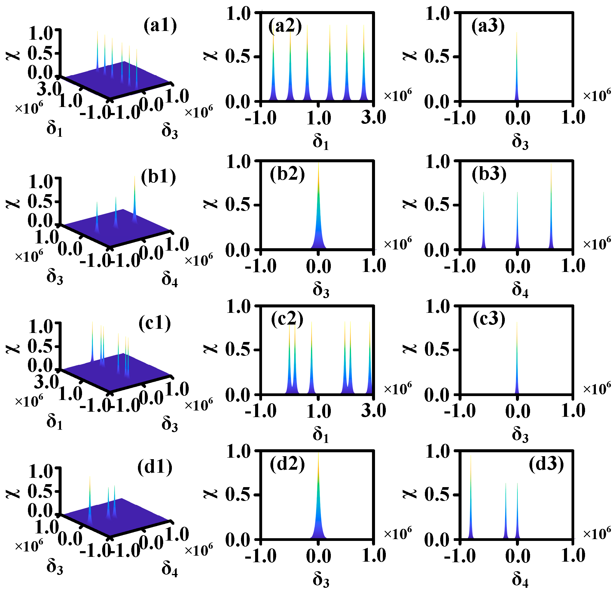
The fifth-order nonlinear susceptibility ${\mathsf{\chi }}_{\mathrm{s}1}^{\left(5\right)}$ exhibits strong dependence on the single-dressing field, and its variation follows a trend qualitatively consistent with the eigenvalue behavior of the coupled system. In Figure 3, two sets of three-dimensional plots display the amplitude distribution of $\left|{\mathsf{\chi }}_{\mathrm{s}1}^{\left(5\right)}\right|$ as functions of detuning variables ${\mathsf{\delta }}_1$ and ${\mathsf{\delta }}_1$. These figures reveal multiple resonant peaks with varying intensities aligned along the respective coordinate axes, indicating a transition in the system’s optical response with respect to the control parameters. In Figure 3(a2,b2) and (a3,b3), distinct patterns emerge along the ${\mathsf{\delta }}_1$- and ${\mathsf{\delta }}_2$-axes, with three and two peaks observed, respectively. These features correspond to the eigenvalue structures on either side of the exceptional point (EP). When ${\mathrm{G}}_2/{\mathsf{\Gamma }}_{21}$ exceeds the EP threshold, the observed peak positions align well with the real-part eigenvalue splitting of ${\mathsf{\delta }}_1$ and ${\mathsf{\delta }}_2$. In contrast, for ${\mathrm{G}}_2/{\mathsf{\Gamma }}_{21}$ below the EP, the imaginary-part contributions become dominant, and the system exhibits features consistent with dissipative phase transitions.

A closer inspection of Figure 3(a3) shows that under strong dressing conditions (${\mathrm{G}}_2/{\mathsf{\Gamma }}_{21}=0.8$), the peak distribution resembles the spectral profile associated with real-part eigenvalue splitting. Conversely, in Figure 3(b3), when the dressing field is weakened (${\mathrm{G}}_2/{\mathsf{\Gamma }}_{21}=0.2$), the peak pattern shifts toward that of imaginary-part splitting, reflecting the dominance of dephasing in this regime. To quantify these effects, the corresponding eigenvalues are extracted as follows: Under real-part dominance, ${\mathsf{\lambda }}_{\mathrm{r}\mathrm{e}1}=0.73 \mathrm{G}\mathrm{H}\mathrm{z}$, ${\mathsf{\lambda }}_{\mathrm{r}\mathrm{e}2}=-0.72 \mathrm{G}\mathrm{H}\mathrm{z}$, ${\mathsf{\lambda }}_{\mathrm{i}\mathrm{m}1}=-0.45 \mathrm{G}\mathrm{H}\mathrm{z}$, ${\mathsf{\lambda }}_{\mathrm{i}\mathrm{m}2}=-0.68 \mathrm{G}\mathrm{H}\mathrm{z}$. These values match the peak positions in the transverse slices of Figure 3(a3,b3), and their origin traces back to the eigenvalue trends displayed in Figure 2c,d. To evaluate the degree of asymmetry between real and imaginary contributions, a symmetry breaking ratio is introduced: ${\mathrm{R}}_{\mathsf{\lambda }}=({\mathsf{\lambda }}_{\mathrm{r}\mathrm{e}1}-{\mathsf{\lambda }}_{\mathrm{r}\mathrm{e}2})/({\mathsf{\lambda }}_{\mathrm{i}\mathrm{m}1}-{\mathsf{\lambda }}_{\mathrm{i}\mathrm{m}2})=1.45/0.23=5.35.$ This indicates that the real-part splitting is over five times greater than the imaginary-part counterpart at the same EP-relative position. Such asymmetry is rooted in the eigenvalue expressions detailed in Table S1–S3 in Supplementary Materials. Specifically, for the real-part splitting to dominate, the conditions Δ ≫ Γ, G ≥ Γ and Δ ≪ Γ, G ≤ Γ must be satisfied, where higher-order terms in Δ and G significantly influence the symmetry structure. Conversely, imaginary-part splitting prevails due to the predominance of the dissipative term Γ. Additionally, the midpoint between the paired peak positions—often corresponding to a spectral dip—represents the destructive interference or “dark state” configuration typically found near the EP. These transitions between bright and dark states further reinforce the interpretation of EP-induced symmetry breaking, offering a direct mapping between spectral features and eigenvalue dynamics in both the coherent and dissipative domains.

In Figure 4, we can see that EP of single-dressing field G2 is ${\mathrm{G}}_2/{\mathsf{\Gamma }}_{21}$= 0.5 In Figure 4(a1), where ${\mathrm{G}}_2/{\mathsf{\Gamma }}_{21}$= 0.8, through the Laplace transform, the two horizontal axes are ${\mathsf{\tau }}_1$ and ${\mathsf{\tau }}_2$, respectively. The highest point is generally located at zero. Figure 4(a2) shows the Rcc of eigenvalue ${\mathsf{\delta }}_1$ on the right side of the EP. When the eigenvalue of ${\mathsf{\delta }}_1$ is on the right side of the EP, the fifth-order nonlinear polarizability of ${\mathsf{\delta }}_1$ has 3 peaks, resulting in 3 cycles in the figure. Multi-period coupling generates complex cosine signals. In Figure 4(a3), ${\mathsf{\delta }}_2$ has two distinct peaks. generating an oscillation period on the image so that it is a simple cosine periodic function with a decaying signal over time, which can be seen from the following formula: $\mathsf{\omega }=2\mathsf{\pi }\mathrm{f}=2\mathsf{\pi }\left|{\mathrm{f}}_1-{\mathrm{f}}_2\right|$.

In Figure 4(b1), where ${\mathrm{G}}_2/{\mathsf{\Gamma }}_{21}$= 0.8, the Rcc of ${\mathsf{\delta }}_1$ on the left side of the EP exchanges resonant position and linewidth compared with the Rcc on the right side of the EP in the simulation diagram. In Figure 4(b2), when the eigenvalue of ${\mathsf{\delta }}_1$ is on the left side of the EP, the gain and loss are interchanged, and there are still three different peaks of the fifth-order nonlinear polarizability, generating three oscillation periods, which presents as the complex cosine signal. Figure 4(b3) shows the Rcc simulation diagram of ${\mathsf{\delta }}_2$ on the left side of the EP. The fifth-order nonlinear polarizability related to eigenvalue ${\mathsf{\delta }}_2$ has two peaks and only produces one oscillation period.

By comparing Figure 4(a2) with Figure 4(b2,a3) and with Figure 4(b3), we can find that the real part has larger oscillation period, the imaginary part obtains a smaller oscillation period; the real part attenuates more slowly, and the imaginary part attenuates more greatly. This is because when the real part is dominant, dressing field strength G leads to oscillation and relaxation time Γ leads to attenuation. When the imaginary part is dominant, Γ leads to oscillation and G leads to attenuation. The splitting effect of the real part is stronger than the imaginary part.

Based on the Rcc expression, we perform numerical simulations of the signal amplitude, temporal periodicity, and coupling behavior under varying intensities of the dressing field. As shown in Figure 1, the exceptional point (EP) associated with the single-dressing field ${\mathrm{G}}_2$ is located at ${\mathrm{G}}_2/{\mathsf{\Gamma }}_{21}$= 0.5. When the field strength is increased to ${\mathrm{G}}_2/{\mathsf{\Gamma }}_{21}$= 0.5, as depicted in Figure 4(a1), the Laplace transform is applied to shift the analysis from the frequency domain to the time domain. The resulting three-dimensional plot uses ${\mathsf{\tau }}_1$ and ${\mathsf{\tau }}_2$ as its horizontal axes, with the global maximum typically appearing near the origin.

In Figure 4(a2), corresponding to the right-hand side of the EP, the Rcc associated with eigenvalue ${\mathsf{\delta }}_1$ exhibits three distinct oscillation periods, reflecting the three-peak structure of its fifth-order nonlinear polarizability $\left|{\mathsf{\chi }}_{\mathrm{s}1}^{\left(5\right)}\right|$. These multiple peaks result in a complex cosine-modulated signal profile, indicative of multi-period coupling dynamics. Meanwhile, Figure 4(a3) presents the Rcc of eigenvalue ${\mathsf{\delta }}_2$, which shows only two sharp peaks, producing a relatively simple cosine oscillation with clear exponential decay. The oscillation frequency can be approximated by the relation $\mathsf{\omega }=2\mathsf{\pi }\mathrm{f}=2\mathsf{\pi }\left|{\mathrm{f}}_1-{\mathrm{f}}_2\right|$, where ${\mathrm{f}}_1$ and ${\mathrm{f}}_2$ are the frequencies corresponding to the two peaks.

In contrast, Figure 4(b1) shows the Rcc of ${\mathsf{\delta }}_1$ when ${\mathrm{G}}_2/{\mathsf{\Gamma }}_{21}$= 0.2, placing the system on the left-hand side of the EP. Compared with the configuration on the right-hand side of the EP, the resonance position and linewidth are interchanged due to the reversal of gain and loss contributions. In Figure 4(b2), the nonlinear polarizability spectrum of δ1\delta_1δ1 continues to display three peaks, resulting in three periodic oscillations in time. The signal maintains a complex cosine structure even under gain–loss inversion. However, in Figure 4(b3), the Rcc for ${\mathsf{\delta }}_2$ shows only two peaks in its nonlinear response and generates a single oscillation period, with a more rapid decay compared to its counterpart in (a3).

By comparing the Rcc in Figure 4(a2,b2,a3,b3), several trends emerge. Signals associated with dominant real parts demonstrate longer oscillation periods and slower attenuation, while those governed by imaginary parts exhibit shorter periods and faster decay. This behavior arises because, under real-part dominance, the dressing field strength G determines the oscillation frequency, whereas the relaxation rate Γ controls attenuation. Conversely, when the imaginary component is dominant, Γ governs the oscillatory behavior and G contributes to the signal’s decay. These results illustrate that the eigenvalue splitting in the real part is more pronounced than that in the imaginary part, leading to more evident oscillatory features in the time domain.

The quantum information capacity can be characterized by the expression n^m, where n denotes the number of entangled photons and mmm represents the number of coherent channels. In the context of this study, with three entangled photons considered, the information capacity increases with the number of available coherent channels. Introducing additional dressing fields enhances the number of these channels, thereby enabling exponential growth in the quantum information capacity.

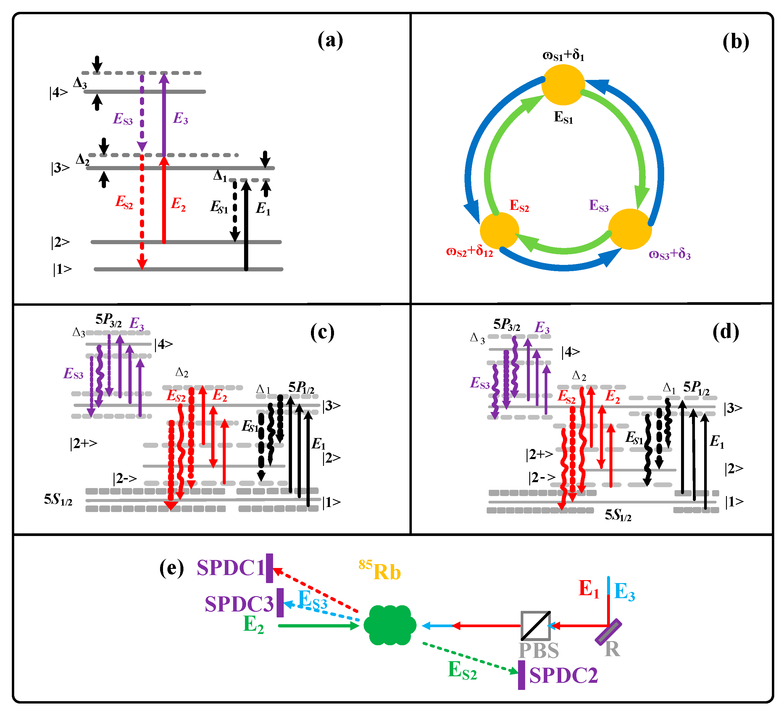
2.2. Parallel Double-Dressing Effect

Considering the multi-dressing effect, the two types of multi-dressing effect that we are studying here are the parallel double-dressing effect and parallel triple-dressing effect. Firstly, the focus is on parallel double-dressing effect. The expression ${\mathsf{\rho }}_{\mathrm{s}3}^{\left(5\right)}$ for q can be written as follows:

$${\chi }_{S1}^{\left(5\right)}={\displaystyle \frac{2N{\mu }_{13}{\mu }_{23}^2{\mu }_{34}^2}{{\epsilon }_0{\hslash }^5}}{\displaystyle \frac{1}{{\mathrm{d}}_1{\mathrm{d}}_2{\mathrm{d}}_3^{\prime }{\mathrm{d}}_4{\mathrm{d}}_5^{\prime }}}$$

(5)

$\mathrm{w}\mathrm{h}\mathrm{e}\mathrm{r}\mathrm{e} {\mathrm{d}}_3^{\mathrm{\prime }}={\mathrm{d}}_3+{{\mathrm{G}}_3}^2/({\mathsf{\Gamma }}_{41}-\mathrm{i}{\mathsf{\delta }}_2-\mathrm{i}{\mathsf{\delta }}_3+i{\mathsf{\Delta }}_2+i{\mathsf{\Delta }}_3).$ In analyzing the influence of the parallel double-dressing configuration, it is important to emphasize that its mathematical structure is formally equivalent to the superposition of two independent single-dressing effects. Following a similar approach to the single-dressing analysis, the complete denominator of Equation (5) is set to zero to solve for the system’s eigenvalues. The corresponding results are systematically presented in Tables S4 and S5 in Supplementary Materials.

Despite this formal equivalence, the physical implications of the double-dressing scenario are more intricate than those of single dressing. This increased complexity stems from the relative spatial and spectral arrangement of the two dressing fields, which introduces distinctions in their mutual priority, degree of coupling, and separability. It is worth emphasizing that in the parallel configuration, the dressing fields function independently, with no mutual coupling between their induced interactions. As a result, from a structural classification standpoint, both the single-dressing and parallel double-dressing scenarios can be interpreted within a consistent theoretical framework. Specifically, the single-dressing case corresponds to a single instance of second-order eigenvalue splitting. whereas the parallel double-dressing manifests as two isolated, second-order splitting—one from each dressing channel.

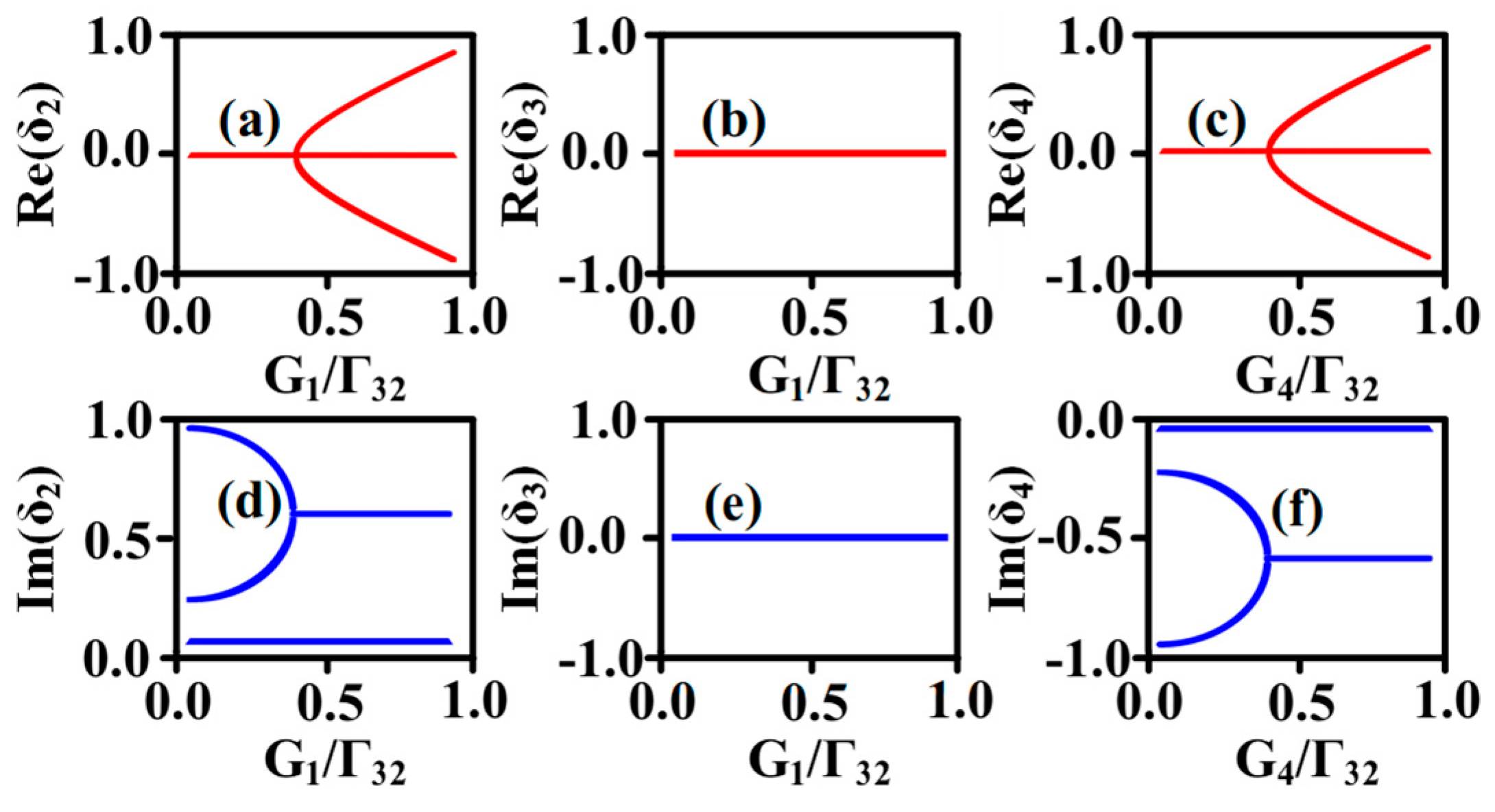
This classification is visually reinforced by Figure 5a–d, which illustrates the splitting behavior of the eigenvalues under the G₂ and G₃ dressing fields. In these figures, the eigenvalues exhibit distinct bifurcation points and phase transitions, further supporting the interpretation that each dressing field independently modulates the system without mutual interference. In Figure 5a, when the value of ${\mathrm{G}}_2/{\mathsf{\Gamma }}_{13}$ is large, eigenvalue ${\mathsf{\delta }}_2$ is on the right-hand side of EP, and the real part of the eigenvalue ${\mathsf{\delta }}_2$ has a splitting effect. ${\mathsf{\delta }}_{1\pm }=(-{2\mathsf{\Delta }}_2+{\mathsf{\Delta }}_3\pm ({\left({2\mathsf{\Delta }}_2+{\mathsf{\Delta }}_3\right)}^2-4({\mathsf{\Delta }}_2{\left({\mathsf{\Delta }}_2+{\mathsf{\Delta }}_3\right)-\mathsf{\Gamma }}_{34}{\mathsf{\Gamma }}_{21}-{{\mathrm{G}}_2}^2){)}^{1/2})/2$ Conversely, in Figure 5b, when the value of ${\mathrm{G}}_2/{\mathsf{\Gamma }}_{13}$ is small, the imaginary part of the eigenvalue ${\mathsf{\delta }}_2$ has a splitting effect. ${\mathsf{\delta }}_{1\pm }=-\mathrm{i}\left({\mathsf{\Gamma }}_{21}+{\mathsf{\Gamma }}_{41}\right)\pm \mathrm{i}\left(\right({\mathsf{\Gamma }}_{21}+{\mathsf{\Gamma }}_{41}{)}^2-4({\mathsf{\Gamma }}_{21}{\mathsf{\Gamma }}_{31}+{{\mathrm{G}}_3}^2){)}^{1/2}/2$.

In the case of parallel double-dressing, the number of coherent channels generated significantly exceeds that of the single-dressing scenario, reaching a total of eight. For the eigenvalue ${\mathsf{\delta }}_3$, which exhibits the highest multiplicity, four of these coherent channels are attributed to the influence of the dressing fields. When analyzing the evolution from energy level splitting governed by a strong dressing field to that driven by a weaker one, and interpreting the exceptional point (EP) as a quasi-superposition state exhibiting coherent channel-like properties, it can be approximated that the number of coherent channels remains constant throughout this transition—matching the EP count of four. This suggests that parallel dressing shares the same quantitative relationship between the number of coherent channels and the number of EPs as observed in the single-dressing scenario. This insight supports the interpretation that parallel double-dressing effectively behaves as a superposition of two independent single-dressing processes. Extending this reasoning, it is plausible to predict that a parallel multi-dressing configuration involving more dressing fields can likewise be viewed as a composite of multiple single-dressing effects.

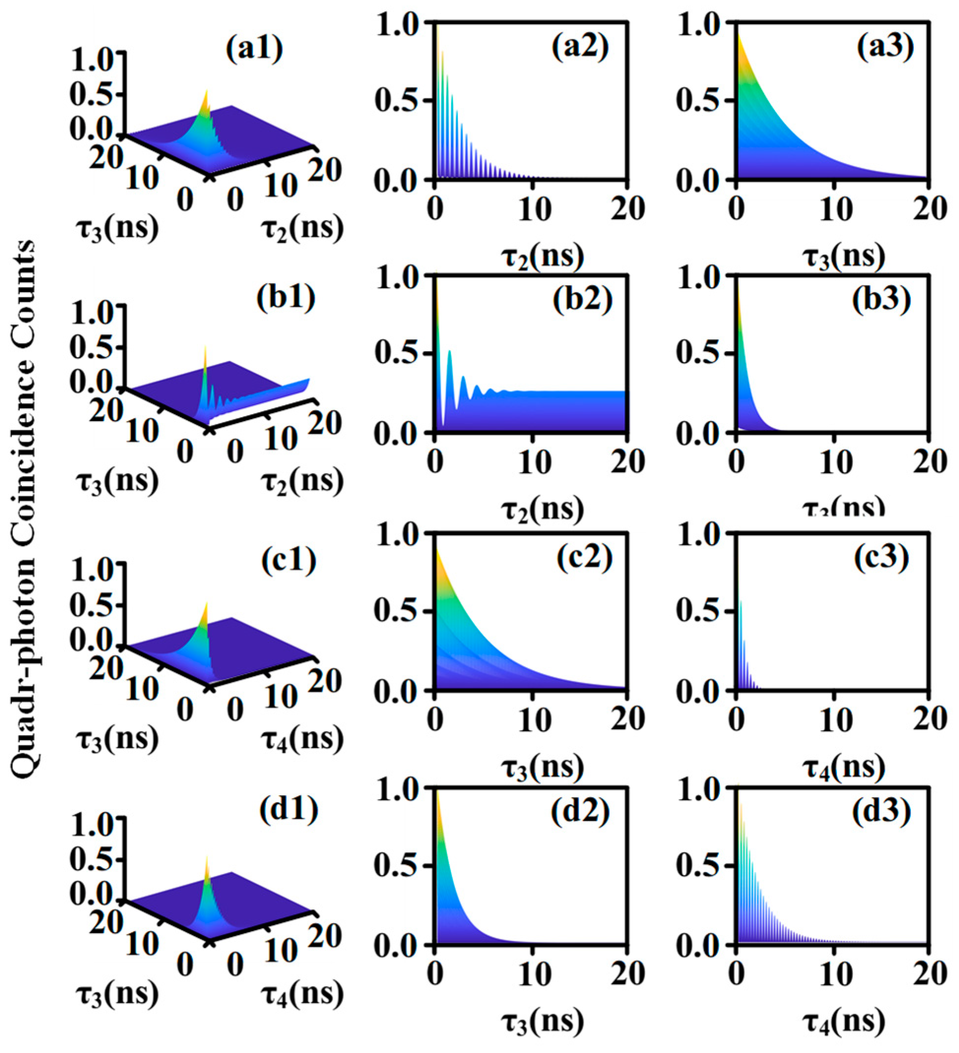
Under the influence of the parallel double-dressing fields ${\mathrm{G}}_2$ and ${\mathrm{G}}_3$, there are different peaks on the simulation images because of two independent dressing fields. Figure 6(a1) shows that when the intensity of the dressing fields ${\mathrm{G}}_2/{\mathsf{\Gamma }}_{21}$ =0.5 and ${\mathrm{G}}_3/{\mathsf{\Gamma }}_{41}$ =0.7, the two eigenvalues are both on the right side of EP, while the fifth-order nonlinear polarizability of the eigenvalues has different number distributions and intensity distributions in the ${\mathsf{\delta }}_1$ and ${\mathsf{\delta }}_2$ directions. The peak pair corresponds to the values obtained by the eigenvalues in Figure 5a,c, when ${\mathrm{G}}_2/{\mathsf{\Gamma }}_{21}$ = 0.5 and ${\mathrm{G}}_3/{\mathsf{\Gamma }}_{41}$= 0.5. As for Figure 6(a2), the four peaks in the figure are the result of the real parts of ${\mathsf{\delta }}_1$ undergoing energy level splitting; their values are ${\mathsf{\lambda }}_1=0.92 \mathrm{G}\mathrm{H}\mathrm{z},{\mathsf{\lambda }}_2 =-0.05 \mathrm{G}\mathrm{H}\mathrm{z},{\mathsf{\lambda }}_3 =-0.65 \mathrm{G}\mathrm{H}\mathrm{z},{\mathsf{\lambda }}_2 =-0.93 \mathrm{G}\mathrm{H}\mathrm{z}$. Figure 6(a3) has the two peaks of the symmetry breaking of ${\mathsf{\delta }}_2$ on the right side of the EP. Their values are ${\mathsf{\lambda }}_1 =1.97 \mathrm{G}\mathrm{H}\mathrm{z},{\mathsf{\lambda }}_2=-1.94 \mathrm{G}\mathrm{H}\mathrm{z}$, $\mathrm{w}\mathrm{h}\mathrm{i}\mathrm{c}\mathrm{h}$ can be observed in Figure 5c, corresponding to the horizontal coordinate of the peak values in Figure 5a–c. In Figure 6(b1), when the dressing field ${\mathrm{G}}_2/{\mathsf{\Gamma }}_{13}$ is less than 0.4 and dressing field ${\mathrm{G}}_2/{\mathsf{\Gamma }}_{21}$ is less than 0.3, and when ${\mathrm{G}}_2/{\mathsf{\Gamma }}_{21}$ = 0.3 and ${\mathrm{G}}_3/{\mathsf{\Gamma }}_{41}$ = 0.2, the imaginary part splits to produce multiple peaks. In Figure 6(b2), the imaginary part of ${\mathsf{\delta }}_2$ dominates to produce four peaks, and the two peaks splitting from the same EPs are relatively close. Compared to Figure 6(b3), when the dressing field ${\mathrm{G}}_3/{\mathsf{\Gamma }}_{41}$ is 0.2 (at the left side of the EPs), the imaginary part’s peak bandwidth of ${\mathsf{\delta }}_2$ is different, with values of −0.91 GHz and −0.93 GHz. The symmetry breaking ratio ${\mathrm{R}}_{\mathsf{\lambda }}$ can be calculated by ${\mathrm{R}}_{\mathsf{\lambda }}=({\mathsf{\lambda }}_{\mathrm{r}\mathrm{e}1}-{\mathsf{\lambda }}_{\mathrm{r}\mathrm{e}4})/\left(\right({\mathsf{\lambda }}_{\mathrm{i}\mathrm{m}1}-{\mathsf{\lambda }}_{\mathrm{i}\mathrm{m}2})/2)=1.94/0.82=2.4.$

Figure 7(b1) shows the simulation diagram of the Rcc when the imaginary part dominates and there is the exchange of resonance position and linewidth when the real part dominates. In Figure 7(b2), when the dominant position is on the left side of the EP, the dispersion and loss are interchangeable, and the ${\mathsf{\delta }}_1$ still has four different peaks, generating six cycles, which is the complex cosine signal. Figure 7(b3) shows the simulation diagram of the Rcc of ${\mathsf{\delta }}_2$ dominated on the left side of the EP. The fifth-order nonlinear polarizability has two peaks and only produces one period.

According to the law of conservation of energy ${\mathsf{\delta }}_1{+\mathsf{\delta }}_2+{\mathsf{\delta }}_3=0$, it can be seen that the maximum number of channels of the tri-photon with the parallel double-dressing effect is 8, and the corresponding eigenvalue is ${\mathsf{\delta }}_3$. Therefore, in this correspondence, in the simulation that conforms to the counting rate, we do not select the eigenvalue with the largest number of cycles for simulation, but according to the law of conservation of energy, we can judge that the largest number of cycles is 28.

2.3. Parallel Triple-Dressing Effect

The expression ${\mathsf{\rho }}_{\mathrm{s}3}^{\left(5\right)}$ for q can be written as follows:

$${\chi }_{S1}^{\left(5\right)}={\displaystyle \frac{2N{\mu }_{13}{\mu }_{23}^2{\mu }_{34}^2}{{\epsilon }_0{\mathrm{\hslash }}^5}}{\displaystyle \frac{1}{{\mathrm{d}}_1{\mathrm{d}}_2{\mathrm{d}}_3^{\mathrm{\prime }}{\mathrm{d}}_4^{\mathrm{\prime }}{\mathrm{d}}_5^{\mathrm{\prime }}}}$$

(6)

where ${\mathrm{d}}_4^{\mathrm{\prime }}={\mathrm{d}}_4+{{\mathrm{G}}_1}^2/({\mathsf{\Gamma }}_{20}+i{\mathsf{\Delta }}_1-\mathrm{i}{\mathsf{\delta }}_1).$ Based on the computational results, it is evident that the presence of the dressing field leads to multi-channel splitting in both the real and imaginary components of the eigenvalue, and the splitting point is EP, which is the same for the real and imaginary parts. When the polarizability reaches the extreme value, the cubic term of the eigenvalue appears in the denominator. For this case, we obtain the corresponding eigenvalue simulation results from same method: we treat parallel triple-dressing effect as three independent single-dressing effects.

The dephasing rate Γ_ij in this paper is similar to the gain/loss in microcavity/waveguide coupling system. In next part, by using the process of six-wave mixing, the theoretical calculations and simulations of the eigenvalues, polarization rates, and conformal count rates of the PT symmetry using the single-dressing effect, the parallel double-dressing effect, as well as the parallel triple-dressing effect have been carried out to analyze the differences and connections between them. It is also found that the maximum number of multi-channels generated increases with the increase in the number of photons and the number of applied parallel dressing fields. Furthermore, the multi-photon correlation can be expanded from the regions of the strong dressing (small dephasing rate) to weak dressing (large dephasing rate).

Compared to the parallel double-dressing fields and single-dressing effect, the parallel triple-dressing setup introduces an additional perturbation field. However, all parallel triple-dressing fields are mutually independent and do not exhibit any sequential or internal–external relationships. In contrast, when compared to the parallel double-dressing fields, two of parallel double-dressing fields simultaneously influence the same eigenvalue, ${\mathsf{\delta }}_1$. Under the influence of these two perturbation fields, ${\mathsf{\delta }}_1$ experiences an energy level splitting. The relative magnitudes of the splitting depend on the interplay between the dressing Rabi frequencies and the dephasing rate, as reflected in the varying degree of level splitting shown in Figure 8a,b,d,e. Additionally, the dressing field G₃ acts independently on the eigenvalue ${\mathsf{\delta }}_3$, yielding results consistent with the single-dressing effect case. The parallel triple-dressing effect adds an additional dimension at the dressing field level, thereby enhancing the quantum information capacity. This suggests that as the number of dressing fields increases, the level splitting brings about more resonant positions, which in turn leads to an increase in the number of coherent channels as the number of dressing fields rises.

A closer inspection of Figure 9(a3) shows that under strong dressing conditions ${\mathrm{G}}_2/{\mathsf{\Gamma }}_{21}=0.3$, the peak distribution resembles the spectral profile associated with real-part eigenvalue splitting. Conversely, in Figure 9(b3), when the dressing field is weakened (${\mathrm{G}}_2/{\mathsf{\Gamma }}_{21}=0.3$), the peak pattern shifts toward that of imaginary-part splitting, reflecting the dominance of dephasing in this regime. To quantify these effects, the corresponding eigenvalues are extracted as follows: under real-part dominance, ${\mathsf{\lambda }}_{\mathrm{r}\mathrm{e}1}=0.73 \mathrm{G}\mathrm{H}\mathrm{z}$, ${\mathsf{\lambda }}_{\mathrm{r}\mathrm{e}2}=-0.72 \mathrm{G}\mathrm{H}\mathrm{z}$, ${\mathsf{\lambda }}_{\mathrm{r}\mathrm{e}3}=0.73 \mathrm{G}\mathrm{H}\mathrm{z}$, ${\mathsf{\lambda }}_{\mathrm{r}\mathrm{e}4}=-0.72 \mathrm{G}\mathrm{H}\mathrm{z}$,${\mathsf{\lambda }}_{\mathrm{i}\mathrm{m}1}=-0.45 \mathrm{G}\mathrm{H}\mathrm{z}$, ${\mathsf{\lambda }}_{\mathrm{i}\mathrm{m}2}=-0.68 \mathrm{G}\mathrm{H}\mathrm{z}$. These values match the peak positions in the transverse slices of Figure 3(a3,b3), and their origin traces back to the eigenvalue trends displayed in Figure 2c,d. To evaluate the degree of asymmetry between real and imaginary contributions, a symmetry breaking ratio is introduced as follows: ${\mathrm{R}}_{\mathsf{\lambda }}=({\mathsf{\lambda }}_{\mathrm{r}\mathrm{e}1}-{\mathsf{\lambda }}_{\mathrm{r}\mathrm{e}2})/({\mathsf{\lambda }}_{\mathrm{i}\mathrm{m}1}-{\mathsf{\lambda }}_{\mathrm{i}\mathrm{m}2})=1.45/0.23=5.35.$

Figure 10(a2) shows the Rcc of δ₁ on the right side of the EP. When positioned to the right of the EP, the eigenvalue δ₁ exhibits four peaks, resulting in six cycles. The multi-period coupling generates a complex cosine signal. In Figure 10(a3), δ₃ displays two distinct peaks, leading to a single cycle, which is a simple cosine periodic function, with its signal decaying over time. Figure 10(b1) shows the Rcc of δ₁ on the left side of the EP, along with the simulated exchange of resonance positions and linewidths compared to the case on the right side of the EP. In Figure 10(b2), when positioned to the left of the EP, dispersion and loss are exchanged. There are still four distinct peaks, resulting in six cycles, corresponding to a complex cosine signal. Figure 10(b3) shows the Rcc simulation of δ₃ on the left side of the EP. The eigenvalue δ₃ exhibits two peaks, generating only one cycle. According to the energy conservation law, it can be deduced that the maximum number of channels in the tri-photon is 8, with the corresponding eigenvalue being δ₂. Based on this, and following the energy conservation law, the maximum number of cycles is determined to be 28.

In summary, as the number of dressing fields increases, the quantum information capacity grows exponentially. Simulations of single-dressing, parallel double-dressing, and parallel triple-dressing schemes demonstrate that the number of exceptional points (EPs) increases accordingly. This results in a doubling of energy level splitting and a corresponding rise in the number of coherent channels. Consequently, the number of peaks in the nonlinear polarization spectra increases, and this enhancement is reflected in the Rcc simulations as a further increase in the number of oscillation periods. These findings highlight the scalability of coherent control and signal complexity in multi-field dressed quantum systems.

3. Basic Theory and Simulation of Quad-Photon System

3.1. Single-Dressing Effect

We also used a beam with detuning ${\mathsf{\Delta }}_1$ as the pump light, as shown in Figure 11. ${\mathit{E}}_1$ (frequency ${\mathit{\omega }}_1$, wave vector ${\mathit{k}}_1$, Rabi frequency ${\mathrm{G}}_1$, wavelength 780 nm, |1> to |3>), ${\mathit{E}}_2$ (${\mathit{\omega }}_2$, ${\mathit{k}}_2$, ${\mathit{G}}_2$, 780 nm, |2> to |4>), ${\mathit{E}}_3$ (${\mathit{\omega }}_3$, ${\mathit{k}}_3$, ${\mathit{G}}_3$, 776 nm, |1> to |4>), ${\mathit{E}}_4$ (${\mathit{\omega }}_4$, ${\mathit{k}}_4$, ${\mathit{G}}_4$, 795 nm, |1> to |4>), with detuning ${\mathsf{\Delta }}_1$, ${\mathsf{\Delta }}_2$, ${\mathsf{\Delta }}_3$, and ${\mathsf{\Delta }}_4$. In the nonlinear optical response to eight-wave mixing, ${\mathit{E}}_{\mathit{s}1}$, ${\mathit{E}}_{\mathit{s}2}$, ${\mathit{E}}_{\mathit{s}3},$ and ${\mathit{E}}_{\mathit{s}4}$, which represent the energy magnitude of the quad-photon and satisfy the energy conservation principle ${\mathsf{\omega }}_1+{\mathsf{\omega }}_2+{\mathsf{\omega }}_3+{\mathsf{\omega }}_4={\mathsf{\omega }}_{\mathrm{s}1}+{\mathsf{\delta }}_1+{\mathsf{\omega }}_{\mathrm{s}2}+{\mathsf{\delta }}_2+{\mathsf{\omega }}_{\mathrm{s}3}+{\mathsf{\delta }}_3+{\mathsf{\omega }}_{\mathrm{s}4}+{\mathsf{\delta }}_4$. A quad-photon system can be described by amplitude $\mathrm{B}({\mathsf{\tau }}_{\mathrm{S}1},{\mathsf{\tau }}_{\mathrm{S}2},{\mathsf{\tau }}_{\mathrm{S}3},{\mathsf{\tau }}_{\mathrm{S}4})$ and the averaged tri-photon coincidence counting rate (Rcc), where $\mathrm{B}({\mathsf{\tau }}_{\mathrm{S}1},{\mathsf{\tau }}_{\mathrm{S}2},{\mathsf{\tau }}_{\mathrm{S}3},{\mathsf{\tau }}_{\mathrm{S}4})$ can be defined as follows:

$$\mathrm{B}\left({\mathsf{\tau }}_1,{\mathsf{\tau }}_2,{\mathsf{\tau }}_3,{\mathsf{\tau }}_4\right)=\mathrm{W}\int \mathrm{d}{\mathsf{\delta }}_1\int \mathrm{d}{\mathsf{\delta }}_2\int \mathrm{d}{\mathsf{\delta }}_3\int \mathrm{d}{\mathsf{\delta }}_4{\mathsf{\chi }}_{\mathrm{S}1}^{\left(7\right)}{\mathrm{e}}^{-\mathrm{i}{\mathsf{\delta }}_1{\mathsf{\tau }}_{12}}{\mathrm{e}}^{-\mathrm{i}{\mathsf{\delta }}_2{\mathsf{\tau }}_{14}}{\mathrm{e}}^{-\mathrm{i}{\mathsf{\delta }}_3{\mathsf{\tau }}_{23}}{\mathrm{e}}^{-\mathrm{i}{\mathsf{\delta }}_3{\mathsf{\tau }}_{13}}$$

(7)

We used Rcc to discuss the temporal correlation of the generated photons. Assuming perfect detection efficiency, Rcc is defined as follows:

$$\mathrm{R}\mathrm{c}\mathrm{c}=\underset{\mathrm{T}\to \mathrm{\infty }}{\mathrm{l}\mathrm{i}\mathrm{m}}{\mathrm{T}}^{-1}{\int }_0^{\mathrm{T}}\mathrm{d}{\mathrm{t}}_{\mathrm{s}1} {\int }_0^{\mathrm{T}}\mathrm{d}{\mathrm{t}}_{\mathrm{s}2}{\int }_0^{\mathrm{T}}\mathrm{d}{\mathrm{t}}_{\mathrm{s}3}{\int }_0^{\mathrm{T}}\mathrm{d}{\mathrm{t}}_{\mathrm{s}4}{\mathrm{G}}^{\left(4\right)}\times {\mathrm{M}}_1({\mathrm{t}}_{\mathrm{s}2}-{\mathrm{t}}_{\mathrm{s}1}){\mathrm{M}}_1({\mathrm{t}}_{\mathrm{s}3}-{\mathrm{t}}_{\mathrm{s}1}){\mathrm{M}}_1({\mathrm{t}}_{\mathrm{s}4}-{\mathrm{t}}_{\mathrm{s}1})$$

(8)

where ${\mathrm{G}}^{\left(4\right)}$ is the fourth-order intensity correlation function of the tri-photon, which can be written as follows: ${\mathrm{G}}^{\left(4\right)}=\left|\mathrm{B}({\mathsf{\tau }}_1,{\mathsf{\tau }}_2,{\mathsf{\tau }}_3,{\mathsf{\tau }}_4{)}^2\right|$. The seventh-order nonlinear susceptibility can be systematically derived through perturbative chain analysis of the spontaneous eight-wave mixing process.

$${\chi }_{S1}^{\left(7\right)}={\displaystyle \frac{2N{\mu }_{20}^2{\mu }_{21}^4{\mu }_{23}^2}{{\epsilon }_0{\hslash }^7}}{\displaystyle \frac{1}{{\mathrm{d}}_1{\mathrm{d}}_2{\mathrm{d}}_3{\mathrm{d}}_4{\mathrm{d}}_5{\mathrm{d}}_6{\mathrm{d}}_7}}$$

(9)

Here, $d_1={\Gamma }_{31}+i{\mathsf{\Delta }}_1$, $d_2={\Gamma }_{42}+i{\mathsf{\Delta }}_2+i{\mathsf{\Delta }}_3$, $d_3={\Gamma }_{32}+i{\delta }_3+i{\mathsf{\Delta }}_2$, $d_4={\Gamma }_{12}-i{\delta }_4-i{\delta }_1$, $d_5={\Gamma }_{32}-i{\delta }_4-i{\delta }_1+i{\mathsf{\Delta }}_1$, $d_6={\Gamma }_{22}-i{\delta }_4$, $d_7={\Gamma }_{32}-i{\delta }_4+i{\mathsf{\Delta }}_4$. When considering the case of single-dressing effect of ${\mathrm{E}}_2$ only, the formula can be written as follows:

$${\chi }_{S1}^{\left(7\right)}={\displaystyle \frac{2N{\mu }_{20}^2{\mu }_{21}^4{\mu }_{23}^2}{{\epsilon }_0{\hslash }^7}}{\displaystyle \frac{1}{{\mathrm{d}}_1{\mathrm{d}}_2{\mathrm{d}}_3{\mathrm{d}}_4{\mathrm{d}}_5{\mathrm{d}}_6^{\mathrm{\prime }}{\mathrm{d}}_7}}$$

(10)

where ${\mathrm{d}}_6^{\mathrm{\prime }}={\mathrm{d}}_6+{{\mathrm{G}}_4}^2/({\mathsf{\Gamma }}_{31}-\mathrm{i}{\mathsf{\delta }}_4+i{\mathsf{\Delta }}_4)$; we calculate the real and imaginary parts of the eigenvalue and the corresponding linewidths by separating the real and imaginary parts. Coherent multi-channel and analytic solutions under various dressing effects are listed in detail in Table S12 of the Supplementary Materials. The main parameters are as follows: ${\Gamma }_{42}=0.5,{\Gamma }_{31}=0.4,{\Gamma }_{41}=0.5,{\Gamma }_{32}=0.5,{\Gamma }_{12}=0.5,{{\Gamma }_{22}=0.5,\mathsf{\Delta }}_1{=0.1,\mathsf{\Delta }}_2=0.2,{\mathsf{\Delta }}_3=0.2{,\mathsf{\Delta }}_3=0.2$.

In Figure 12c, when the dressing Rabi frequency is dominant as ${\mathrm{G}}_4/{\mathsf{\Gamma }}_{32}$ is greater than 0.5, two branches of ${\mathsf{\delta }}_4$ generate two splits at the same time. In Figure 12e, when the dephase rate of ${\mathsf{\delta }}_2$ is dominant as ${\mathrm{G}}_4/{\mathsf{\Gamma }}_{32}$ is less than 0.5, the phase transition is easier to occur. In Figure 12a,c, it can be observed that, according to Figure 11b,c, eigenvalue δ₁ is not directly influenced by the external dressing field G₄, but also the dressing field G₄ acting on eigenvalue δ₄, causing energy level splitting at positions where it would not typically occur.

Figure 11. (a) Energy level diagram of the four-level configuration in 85Rb vapor and the corresponding quad-photon generation process. (b) Spatial alignment scheme of the optical beams used for quad-photon generation in the SEWM process. (c) Illustration of multi-channel formation on the right side of the exceptional point (EP), induced by the Rabi dressing frequency in the SEWM system under single dressing. (d) Multi-channel splitting on the left side of the EP, driven by the Rabi dephasing rate in the SEWM configuration with single dressing. (e) Schematic representation of a simplified experimental setup designed for the spontaneous eight-wave mixing system.

Figure 11. (a) Energy level diagram of the four-level configuration in 85Rb vapor and the corresponding quad-photon generation process. (b) Spatial alignment scheme of the optical beams used for quad-photon generation in the SEWM process. (c) Illustration of multi-channel formation on the right side of the exceptional point (EP), induced by the Rabi dressing frequency in the SEWM system under single dressing. (d) Multi-channel splitting on the left side of the EP, driven by the Rabi dephasing rate in the SEWM configuration with single dressing. (e) Schematic representation of a simplified experimental setup designed for the spontaneous eight-wave mixing system.

This results in second-order energy level splitting that is different from the single-dressing case. This outcome is also consistent with the calculations of the coherent channels. The phenomenon arises because, in the seventh-order nonlinear polarizability, there is an interaction between two eigenvalues, which leads to the extension of the dressing field effects. Due to the low electron efficiency and strong dressing effect in the four-photon process, even undressed eigenvalues can exhibit a strong dressing effect when influenced by other dressed eigenvalues. In simulations of single-dressed eigenvalues, we observed a parallel double dressing effect in another eigenvalue due to energy conservation. This suggests that this effect can be used to induce a dressing effect in energy levels that are otherwise difficult to dress.

In Figure 13, ${\mathsf{\lambda }}_{\mathrm{r}\mathrm{e}1}$ to ${\mathsf{\lambda }}_{\mathrm{r}\mathrm{e}6}$ and ${\mathsf{\lambda }}_{\mathrm{i}\mathrm{m}1}$ to ${\mathsf{\lambda }}_{\mathrm{i}\mathrm{m}6}$ are the eigenvalues of the dressing Rabi frequency (de-phase rate) dominated by the single-dressing fields. Their values are ${\mathsf{\lambda }}_{\mathrm{r}\mathrm{e}1}=-0.84 \mathrm{G}\mathrm{H}\mathrm{z}$, ${\mathsf{\lambda }}_{\mathrm{r}\mathrm{e}2}=-0.47 \mathrm{G}\mathrm{H}\mathrm{z}$, ${\mathsf{\lambda }}_{\mathrm{r}\mathrm{e}3}=-0.21 \mathrm{G}\mathrm{H}\mathrm{z}$, ${\mathsf{\lambda }}_{\mathrm{r}\mathrm{e}4}=1.22 \mathrm{G}\mathrm{H}\mathrm{z}$, ${\mathsf{\lambda }}_{\mathrm{r}\mathrm{e}5}=2.13 \mathrm{G}\mathrm{H}\mathrm{z}$, ${\mathsf{\lambda }}_{\mathrm{r}\mathrm{e}6}=2.75 \mathrm{G}\mathrm{H}\mathrm{z}$, ${\mathsf{\lambda }}_{\mathrm{i}\mathrm{m}1}=-0.12 \mathrm{G}\mathrm{H}\mathrm{z}$, ${\mathsf{\lambda }}_{\mathrm{i}\mathrm{m}2}=-0.09 \mathrm{G}\mathrm{H}\mathrm{z}$, ${\mathsf{\lambda }}_{\mathrm{i}\mathrm{m}3}=0.95 \mathrm{G}\mathrm{H}\mathrm{z}$, ${\mathsf{\lambda }}_{\mathrm{i}\mathrm{m}4}=1.87 \mathrm{G}\mathrm{H}\mathrm{z}$, ${\mathsf{\lambda }}_{\mathrm{i}\mathrm{m}5}=1.94 \mathrm{G}\mathrm{H}\mathrm{z}$, and ${\mathsf{\lambda }}_{\mathrm{i}\mathrm{m}6}=2.89 \mathrm{G}\mathrm{H}\mathrm{z}$, which can be observed in Figure 12a–c, corresponding to the horizontal coordinate of the peak values in Figure 13(a2,c2). The symmetry breaking ratio ${\mathrm{R}}_{\mathsf{\lambda }}$ can be calculated by ${\mathrm{R}}_{\mathsf{\lambda }}=({\mathsf{\lambda }}_{\mathrm{r}\mathrm{e}3}-{\mathsf{\lambda }}_{\mathrm{r}\mathrm{e}5})/\left(\right({\mathsf{\lambda }}_{\mathrm{i}\mathrm{m}1}-{\mathsf{\lambda }}_{\mathrm{i}\mathrm{m}2})/2)=0.86/0.34=2.36.$ According to the relevant calculation of the symmetry breaking ratio, the real part accounts for 2 times more than the imaginary part.

In the temporal evolution of eigenvalue ${\mathsf{\delta }}_3$, a single peak is observed without any cyclic behavior, indicating that it follows a monotonically decaying trend. As shown in Figure 14(c3), the eigenvalue ${\mathsf{\delta }}_4$ displays three prominent peaks, corresponding to three oscillation periods, which characterizes it as a damped periodic function resembling a decaying cosine waveform.

The temporal response patterns of the other eigenvalues in the Rcc numerical simulation exhibit similar features. Specifically, in Figure 14(b3), when the system is situated on the left side of the exceptional point (EP), a role reversal between dispersion and dissipation occurs. In this regime, ${\mathsf{\delta }}_3$ maintains its single-peak profile with an exponentially decaying response, while ${\mathsf{\delta }}_4$ consistently shows three oscillatory peaks, indicating the presence of three distinct temporal cycles. According to the energy conservation law, it can be deduced that the maximum number of channels in the quad-photon with single-dressing field is 6. Based on this, and following the energy conservation law, the maximum number of cycles is determined to be 15.

3.2. Parallel Double Dressing Effect

Firstly, the focus is on parallel double dressing effect. The expression of seventh-order nonlinear polarizability ${\chi }_{S1}^{\left(7\right)}$ can be written as follows:

$${\chi }_{S1}^{\left(7\right)}={\displaystyle \frac{2N{\mu }_{20}^2{\mu }_{21}^4{\mu }_{23}^2}{{\epsilon }_0{\hslash }^7}}{\displaystyle \frac{1}{{\mathrm{d}}_1{\mathrm{d}}_2{\mathrm{d}}_3{\mathrm{d}}_4^{\prime }{\mathrm{d}}_5{\mathrm{d}}_6^{\prime }{\mathrm{d}}_7}}$$

(11)

${\mathrm{w}\mathrm{h}\mathrm{e}\mathrm{r}\mathrm{e} \mathrm{d}}_6^{\prime }={\mathrm{d}}_6+{{\mathrm{G}}_1}^2/({\mathsf{\Gamma }}_{21}-\mathrm{i}{\mathsf{\delta }}_1+i{\mathsf{\Delta }}_1)$; the parallel double-dressing effect is equivalent in formula form to two single-dressing effects. Coherent multi-channel and analytic solutions under various dressing effects are listed in detail in Table S12 of the Supplementary Materials.

The quad-photon and tri-photon parallel double-dressing configurations demonstrate comparable dynamical characteristics when influenced by external perturbative fields, and can both be effectively modeled as systems driven by two distinct perturbation sources. Nonetheless, the seventh-order nonlinear optical response introduces an additional eigenvalue dimension relative to the fifth-order response. This added dimensionality results in a wider distribution of perturbation-sensitive regions and leads to altered coupling mechanisms among the underlying nonlinear processes. Figure 15a,d illustrates that the eigenvalue ${\mathsf{\delta }}_2$ undergoes a phase transition at a specific ratio between the dressing field strength and the dephasing rate, exhibiting behavior analogous to that observed in the single-dressing configuration. Similarly, Figure 15c,f reveals the presence of an exceptional point (EP) in the eigenvalue ${\mathsf{\delta }}_4$, which arises from the interplay between the dressing field and the dephasing dynamics.

Figure 16 presents the simulated results of seventh-order nonlinear susceptibility under parallel double-dressing conditions, evaluated across different eigenvalue dimensions. The corresponding ratios of dressing field strength to dephasing rate are specified as follows: for the regime to the right of the exceptional point (EP), ${\mathrm{G}}_1/{\mathsf{\Gamma }}_{32}=0.6$, ${\mathrm{G}}_4/{\mathsf{\Gamma }}_{32}=0.6$; for the regime to the left of the EP, ${\mathrm{G}}_1/{\mathsf{\Gamma }}_{32}=0.2$, ${\mathrm{G}}_4/{\mathsf{\Gamma }}_{32}=0.2$. In Figure 16, groups (a) and (b) illustrate the influence of the dressing fields on the peak wavelength of the polarization response, corresponding, respectively, to the eigenvalue dimensions along directions ${\mathsf{\delta }}_1$ and ${\mathsf{\delta }}_4$ when situated on the right side of the EP. Their values are ${\mathsf{\lambda }}_{\mathrm{r}\mathrm{e}1}=-0.77 \mathrm{G}\mathrm{H}\mathrm{z}$, ${\mathsf{\lambda }}_{\mathrm{r}\mathrm{e}2}=0.06 \mathrm{G}\mathrm{H}\mathrm{z}$, and ${\mathsf{\lambda }}_{\mathrm{r}\mathrm{e}3}=0.76 \mathrm{G}\mathrm{H}\mathrm{z}$. In contrast, the figure groups (c) and (d) represent the polarization peak wavelength response in the eigenvalue directions 1 and 4, respectively, for the regime on the left side of the EP. Their values are ${\mathsf{\lambda }}_{\mathrm{i}\mathrm{m}1}=0.35 \mathrm{G}\mathrm{H}\mathrm{z}$, ${\mathsf{\lambda }}_{\mathrm{i}\mathrm{m}2}=0.56 \mathrm{G}\mathrm{H}\mathrm{z}$, and ${\mathsf{\lambda }}_{\mathrm{i}\mathrm{m}3}=0.79 \mathrm{G}\mathrm{H}\mathrm{z}$.

Figure 17 illustrates the Rcc-damped Rabi oscillations arising under varying numbers and positions of peaks in the susceptibility spectrum. When the susceptibility exhibits three distinct peaks, it corresponds to a damped Rabi oscillation with three periods, where the decay rates are governed by the coupling of the imaginary parts of three eigenvalues (left side of the exceptional point, EP). On the right side of the EP, the number of oscillation periods remains unchanged; however, an interchange between the real and imaginary parts occurs, manifesting as alterations in the oscillation period and decay rate observed in the corresponding figures. When only a single peak is present, it indicates the existence of only one coherent channel, which is insufficient to produce oscillations. According to the energy conservation law, it can be deduced that the maximum number of channels in the quad-photon with double dressing field is 16. Based on this, and following the energy conservation law, the maximum number of cycles is determined to be 36.

3.3. Parallel Triple-Dressing Effect

The expression ${\chi }_{S1}^{\left(7\right)}$ for parallel triple-dressing effect can be written as follows:

$${\chi }_{S1}^{\left(7\right)}={\displaystyle \frac{2N{\mu }_{20}^2{\mu }_{21}^4{\mu }_{23}^2}{{\epsilon }_0{\hslash }^7}}{\displaystyle \frac{1}{{\mathrm{d}}_1{\mathrm{d}}_2{\mathrm{d}}_3{\mathrm{d}}_4^{\prime }{\mathrm{d}}_5{\mathrm{d}}_6^{\prime }{\mathrm{d}}_7^{\prime }}}$$

(12)

where ${\mathrm{d}}_7^{\prime }={\mathrm{d}}_7+{{\mathrm{G}}_3}^2/({\mathsf{\Gamma }}_{31}-\mathrm{i}{\mathsf{\delta }}_1+i{\mathsf{\Delta }}_1+i{\mathsf{\Delta }}_3)$; coherent multi-channel and analytic solutions under various dressing effects are listed in detail in Table S16 of the Supplementary Materials.

Figure 18 shows the eigenvalue simulation for the four-photon parallel three-dressing system. The eigenvalue simulation for the quad-photon parallel tri-dressing system is similar to the three-photon case. The energy level splitting behavior follows the same pattern as that of single dressing. The EP positions corresponding to the three dressing fields are, respectively, as follows: ${\mathrm{G}}_1/{\mathsf{\Gamma }}_{21}=0.25$, ${\mathrm{G}}_3/{\mathsf{\Gamma }}_{31}=0.15$, ${\mathrm{G}}_2/{\mathsf{\Gamma }}_{21}=0.1$.

Figure 19 presents the simulated results of seventh-order nonlinear susceptibility under parallel double-dressing conditions, evaluated across different eigenvalue dimensions. The corresponding ratios of dressing field strength to dephasing rate are specified as follows: for the regime to the right of the exceptional point (EP), ${\mathrm{G}}_1/{\mathsf{\Gamma }}_{21}=0.4$, ${\mathrm{G}}_3/{\mathsf{\Gamma }}_{31}=0.25$, ${\mathrm{G}}_2/{\mathsf{\Gamma }}_{21}=0.15$.; for the regime to the left of the EP, ${\mathrm{G}}_1/{\mathsf{\Gamma }}_{21}=0.1$, ${\mathrm{G}}_3/{\mathsf{\Gamma }}_{31}=0.05$, ${\mathrm{G}}_2/{\mathsf{\Gamma }}_{21}=0.05$. In Figure 19, groups (a) and (b) illustrate the influence of the dressing fields on the peak wavelength of the polarization response, corresponding, respectively, to the eigenvalue dimensions along directions ${\mathsf{\delta }}_1$ and ${\mathsf{\delta }}_4$ when situated on the right side of the EP. Their values are ${\mathsf{\lambda }}_{\mathrm{r}\mathrm{e}1}=-0.97 \mathrm{G}\mathrm{H}\mathrm{z}$, ${\mathsf{\lambda }}_{\mathrm{r}\mathrm{e}2}=-0.84 \mathrm{G}\mathrm{H}\mathrm{z}$, ${\mathsf{\lambda }}_{\mathrm{r}\mathrm{e}3}=0.89\mathrm{z}$, and ${\mathsf{\lambda }}_{\mathrm{r}\mathrm{e}4}=0.98 \mathrm{G}\mathrm{H}\mathrm{z}$. In contrast, the figure groups (c) and (d) represent the polarization peak wavelength response in the eigenvalue directions 1 and 4, respectively, for the regime on the left side of the EP. Their values are ${\mathsf{\lambda }}_{\mathrm{i}\mathrm{m}1}=-0.08 \mathrm{G}\mathrm{H}\mathrm{z}$, ${\mathsf{\lambda }}_{\mathrm{i}\mathrm{m}2}=-0.24 \mathrm{G}\mathrm{H}\mathrm{z}$, ${\mathsf{\lambda }}_{\mathrm{i}\mathrm{m}3}=-0.37 \mathrm{G}\mathrm{H}\mathrm{z}$, and ${\mathsf{\lambda }}_{\mathrm{i}\mathrm{m}4}=-0.49 \mathrm{G}\mathrm{H}\mathrm{z}$.

Figure 20 presents Rcc simulation results similar to those shown in Figure 17, where damped Rabi oscillations arise through the interchange of the real and imaginary components of the eigenvalues, effectively swapping the oscillation period and decay rate. However, a key difference emerges when four coherent channels are involved: in this case, six oscillation periods are theoretically generated. Due to coupling interactions among the oscillation modes, not all six periods can be fully resolved in the observable signal. Nevertheless, a noticeable increase in the number of oscillation cycles—compared to the case with only three coherent channels—is evident, indicating the enhanced complexity of the coherent dynamics. According to the energy conservation law, it can be deduced that the maximum number of channels in the quad-photon with a triple-dressing field is 12. Based on this, and following the energy conservation law, the maximum number of cycles is determined to be 66.

Overall, compared to the tri-photon system, the quad-photon system exhibits an exponential increase in quantum information capacity. This enhancement arises from the higher photon count, which expands the dimensionality of coherent channels. Consequently, the number of Rabi oscillation cycles—each capable of carrying quantum information through pairwise coherence among the channels—increases correspondingly. This indicates that the quantum information capacity of atom-based systems can be significantly improved using this approach.

4. Conclusions and Discussion

This paper systematically investigates the tri-photon interaction scheme involving wavelengths of 780 nm, 780 nm, and 795 nm, as well as the quad-photon interaction configuration comprising 780 nm, 780 nm, 795 nm, and 795 nm within the energy level structure of 85Rb atoms. The influence of different dressing configurations—namely single-dressing, parallel double-dressing, and parallel triple-dressing—on high-order nonlinear optical processes is analytically explored. Through a rigorous mathematical framework, we analyzed the evolution patterns of system eigenvalues, the fifth-order and seventh-order nonlinear polarizabilities, and the behavior of random coincidence counts under varying Rabi frequencies and dephasing rates. Building upon prior theoretical results, this work further contrasts the characteristics of the real and imaginary components of the eigenvalues across the three dressing scenarios. A detailed correspondence is established between the number of eigenvalue branches and the number of resonance peaks in the seventh-order nonlinear polarizability, as well as the variation trends observed in the Rcc oscillation periods. These findings reveal the significant role played by the dressing field in modulating the system’s parity–time (PT) symmetric properties across both temporal and spectral domains, as well as across both Hermitian (real part) and non-Hermitian (imaginary part) dimensions. In essence, the results provide a unified perspective on how multi-photon dressing affects energy-level splitting, coherence pathways, and nonlinear optical responses in complex atomic systems, offering valuable insights into the control of light–matter interactions in non-Hermitian quantum optics.

This study initiates with numerical simulations focused on the physical behavior near non-Hermitian exceptional points (EPs), aiming to explore their controllability. By systematically varying the ratio between the Rabi frequency and the dephasing rate, a clear eigenvalue bifurcation phenomenon is observed at the EP, which signals the onset of energy level splitting in the system. A key observation is that the real components of the eigenvalues demonstrate more pronounced symmetry breaking effects than their imaginary counterparts. This asymmetry indicates that, in regimes where the dephasing rate prevails over the Rabi frequency, the imaginary part becomes the primary contributor to eigenvalue splitting. Such behavior corresponds to out-of-phase destructive dressing mechanisms, which are characterized by nonlocality, degeneracy, non-Abelian properties, and a highly symmetric pattern of symmetry breaking. These findings underscore the intricate interplay between gain-loss mechanisms and coherent interactions in PT-symmetric quantum systems. We conducted a comparative analysis of the simulations of the fifth-order and seventh-order nonlinear optical responses. We found that, in terms of quantum information capacity, the quad-photon process exhibits an exponential increase compared to the three-photon process. The quantum information capacity is given by n^m, where n represents the number of coherent channels and m denotes the number of photons. This is reflected in the increased number of coherent channels and resonant positions. The tri-photon process involves 12 coherent channels and 8 resonant positions, whereas the four-photon process shows an increase to 16 coherent channels and 10 resonant positions. This property is manifested in the number and position of peaks in the polarizability, as well as the number of oscillation periods in the random coincidence counting rate. The maximum number of oscillation periods for the tri-photon process is 6, while for the quad-photon process, it reaches 18.

Finally, we discovered that due to the low electron efficiency and strong dressing effect in the four-photon process, even undressed eigenvalues can exhibit a strong dressing effect when influenced by other dressed eigenvalues. In simulations of single-dressed eigenvalues, we observed a parallel double-dressing effect in another eigenvalue due to energy conservation. This suggests that this effect can be used to induce a dressing effect in energy levels that are otherwise difficult to dress.