Numerical Background-Oriented Schlieren for Phase Reconstruction and Its Potential Applications

Abstract

This study presents a comprehensive numerical framework for Background-Oriented Schlieren (BOS) to systematically evaluate its performance and reconstructive capabilities under complex flow conditions. This framework integrates two stages: forward modeling, using ray tracing to simulate image degradation, and inverse processing, using optical flow and a conjugate gradient algorithm to extract displacements and reconstruct phase information. This method is first validated using turbulent flow fields in the Johns Hopkins Turbulence Database, where the reconstructed phase screens closely match the original data, with relative errors below 4% and structural similarity indices above 0.75 in all cases, providing a possible restoration method for degraded flow field images. It is then applied to shock wave fields with varying Mach numbers; this method achieves meaningful reconstruction at short ranges but fails under long-range imaging due to severe wavefront distortions. However, even in degraded conditions, the extracted optical flow fields preserve structural features correlated with the underlying shock patterns, indicating potential for BOS-based target recognition. These findings highlight both the capabilities and limitations of BOS and suggest new pathways for extending its use beyond traditional flow visualization.

1. Introduction

The propagation of optical waves through the atmosphere presents a formidable challenge for a wide range of applications, including free-space communications, remote sensing, and long-range imaging [1,2,3]. The primary sources of optical degradation can be broadly categorized into two mechanisms: absorption and scattering by aerosols [4,5,6,7] and wavefront distortion induced by refractive index fluctuations in turbulence [8,9,10]. While both mechanisms are significant, this study focuses on the latter, as it dominates in high-speed aerodynamics and is prevalent in scenarios involving temperature or density gradients [11,12,13]. To account for wavefront distortion, researchers often utilize phase screens as inputs in adaptive optics systems, beam-shaping algorithms, and numerical simulations of light propagation [14,15]. However, traditional phase screen models are largely based on theoretical turbulence spectra, such as the Kolmogorov or Von Kármán models [14]. Although widely used, they often fail to reflect the actual complexity and dynamics of real-world flow fields.

An alternative, data-driven approach is provided by Background Oriented Schlieren (BOS), an optical method for visualizing and quantifying refractive index variations by tracking the displacements of the background pattern as light passes through a transparent medium [16,17,18,19,20]. Its non-intrusive nature, compatibility with large-scale experimental setups, and ability to capture fine optical distortions have led to its broad adoption in applications such as helicopter tip vortices, supersonic jets, and combustion flows, the aerodynamic optical effects, and so on [21,22,23,24,25,26]. Despite the excellent performance in flow diagnostics, its potential for reconstructing phase screens remains relatively underexplored. Furthermore, in real-world scenarios involving strong refractive gradients or long-distance imaging, optical distortions can become so severe that they decrease BOS performance. This highlights the need for a systematic evaluation of BOS performance under degraded imaging conditions.

To address these limitations, this study presents a numerical BOS framework that combines forward simulation with reverse reconstruction. The forward simulation models the interaction of light rays with a given flow field, using ray tracing and high-resolution imaging techniques to generate synthetic degraded images. The reverse reconstruction then employs optical flow algorithms, specifically the Farneback method, to extract displacement fields, followed by a conjugate gradient solver to reconstruct optical path differences and the corresponding phase screen. This modular pipeline allows us to systematically analyze how BOS behaves under varying flow structures and imaging geometries and to explore its potential in downstream tasks beyond flow visualization. We apply the proposed framework to two representative flow scenarios: a turbulent flow from the Johns Hopkins Turbulence Database (JHTDB) and a set of compressible shock wave fields at varying Mach numbers. The results reveal both the framework’s accuracy in ideal conditions and its limitations under severe optical distortion.

This paper is organized as follows: Section 2 provides an overview of the BOS principle and a related optical principle. Section 3 introduces the numerical BOS framework. Section 4 presents validation experiments of JHTDB flow regimes, accompanied by qualitative and quantitative analyses. Section 5 discusses the scenarios in which shock fields can be used for phase reconstruction and displacement detection. Finally, Section 6 analyzes and discusses the relevant conclusions and proposed future research directions. Section 7 summarizes the main work of this paper.

2. Principle of the Method

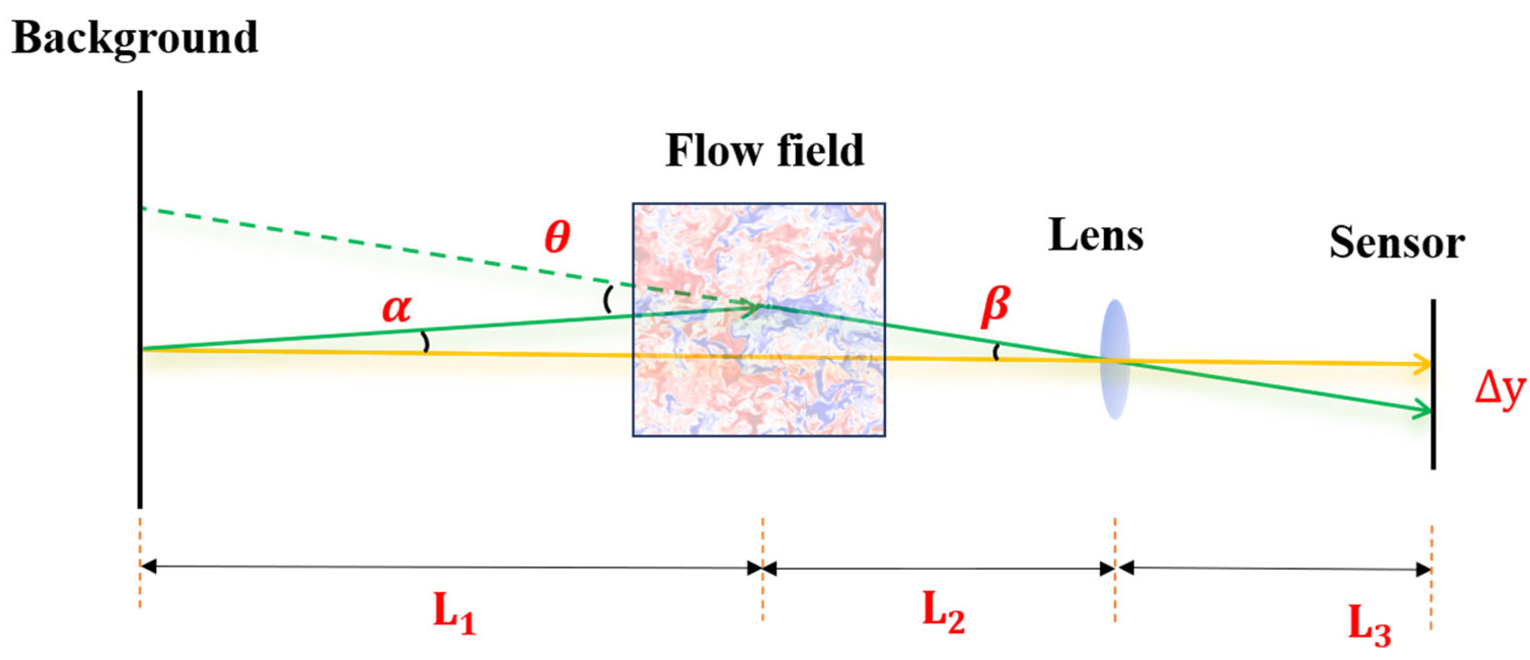
BOS is an optical measurement technique that leverages the distortion of a background image to infer refractive index variations within a flow field. As illustrated in Figure 1, a typical BOS system consists primarily of three components: the background pattern, the disturbed flow field, and the imaging system. It captures and compares background images before and after passing through a flow field to analyze pixel variations, enabling the calculation of flow field information, which has the advantages of simple hardware, low cost, and a wide field of view.

As light passes through the flow field, the variations in the medium’s refractive index gradients cause angular deflections in the trajectories of light rays originating from the background pattern. These deflected rays propagate through the imaging system and are recorded by the CCD sensor, where their positional shifts are captured as image deviations, representing the cumulative effect of refractive index gradients along the light’s path.

Assuming small deflection angles, the angular deviation $\theta$ of a light ray can be linearly approximated as

$$\theta \approx \tan \theta =\tan (\alpha +\beta )$$

(1)

Based on the geometrical configuration of the BOS setup, we derive

$$\begin{array}{c}{L}_1\tan \alpha =L_2\tan \beta \\ \tan \beta ={\displaystyle \frac{\mathrm{\Delta }y}{L_3}},{\displaystyle \frac{1}{f}}={\displaystyle \frac{1}{L_1+L_2}}+{\displaystyle \frac{1}{L_3}}\end{array}$$

(2)

The deflection angle is then given by

$$\theta =(1+{\displaystyle \frac{L_2}{L_1}}){\displaystyle \frac{\mathrm{\Delta }y}{L_3}}={\displaystyle \frac{L_1+L_2-f}{L_{1}f}}\mathrm{\Delta }y$$

(3)

Here, $\mathrm{\Delta }y$ is the measured pixel displacement on the image sensor, and $f$ is the lens focal length. On the other hand, the Optical Path Difference (OPD) is the integral of the refractive index along the light propagation path $L$:

$$OPD(x,y)={\displaystyle \int \left[n(x,y,z)-n_0\right]dz}$$

(4)

While the deflection angle is directly related to the gradient of OPD:

$$\begin{array}{l}{\theta }_x(x,y)={\displaystyle \frac{1}{n_0}}{\displaystyle \frac{\partial OPD(x,y)}{\partial x}}\\ {\theta }_y(x,y)={\displaystyle \frac{1}{n_0}}{\displaystyle \frac{\partial OPD(x,y)}{\partial y}}\end{array}$$

(5)

where $n_0$ is the refractive index of the surrounding medium. If $\mathrm{\Phi }(x,y)$ represents OPD, then Equation (5) can be written as

$$\nabla \mathrm{\Phi }=\theta$$

(6)

By further calculating the partial derivatives of Equation (6) with respect to the spatial coordinates and adding them together, the two-dimensional Laplacian operator form of the OPD can be obtained:

$${\nabla }^2\mathrm{\Phi }={\displaystyle \frac{{\partial }^2\mathrm{\Phi }}{\partial x^2}}+{\displaystyle \frac{{\partial }^2\mathrm{\Phi }}{\partial y^2}}=n_0\left({\displaystyle \frac{\partial {\theta }_x}{\partial x}}+{\displaystyle \frac{\partial {\theta }_y}{\partial y}}\right)$$

(7)

Under the premise of approximately uniform background refractive index, the environmental refractive index is defined as $n_0=1$. Therefore, the governing equation between OPD and deflection angle is

$${\nabla }^2\mathrm{\Phi }=\nabla \cdot \theta$$

(8)

This equation is essentially a two-dimensional Poisson’s equation with a divergence term. The scalar field $\mathrm{\Phi }(x,y)$ can be reconstructed from the measured gradient field $\theta (x,y)$ through numerical iteration.

From the perspective of wave optics, the deflection of light rays in a refractive medium is closely associated with the phase screen $\varphi (x,y)$, which quantifies the cumulative phase delay introduced by variations in the refractive index along the light’s path. This concept is fundamental to wavefront-based modeling and reconstruction in BOS applications. The phase screen can be generally defined as

$$\varphi (x,y)={\displaystyle \frac{2\pi }{\lambda }}OPD$$

(9)

where $\lambda$ is the wavelength of the light, and in the natural light BOS system, the value is $550 \mathrm{nm}$ of the central wavelength of visible light. Based on Equations (3), (8), and (9), the deflection angle serves as a bridge, providing a method for converting pixel displacement into OPD gradient and calculating the phase screen.

3. Simulation Framework

Due to the constantly changing actual flow field, it is difficult to control and obtain accurate flow field information. To achieve a controlled evaluation of the BOS-based phase screen reconstruction process, we developed a simulation-based method. The proposed methodology consists of two key components: forward modeling and reverse reconstruction, which are essentially inverse processes. As shown in Figure 2, forward modeling simulates the generation of degraded images by applying ray tracing to simulate how light rays propagate the flow field. In contrast, reverse reconstruction utilizes the difference between the original image and the degraded image to generate the phase screen and recover the flow field characteristics. These two processes are mutually dependent and enhance the robustness and applicability of the reconstruction method in real-world scenarios.

3.1. Forward Modeling

In order to simulate the image degradation process caused by a flow field, a detailed forward simulation approach is employed. This approach simulates the interaction of light rays with the flow field and the subsequent distortion that occurs as light propagates through a medium with refractive index variations. This process follows a series of steps designed to accurately model the physical phenomena, including light generation, ray tracing through the flow field, and the influence of optical elements on the rays with reference to the work of Rajendran et al. [27]. The procedure is outlined as follows:

3.1.1. Light Ray Generation

Unlike traditional point or collimated sources, our BOS employs a high-contrast background pattern where each pixel effectively serves as an independent emitter, as shown in Figure 3. Rays are generated from these background points and directed toward the camera based on its perspective geometry. The intensity of each ray is determined by the brightness of its corresponding source point. Ideally, each source point could emit an infinite number of rays converging toward the camera’s lens. However, to balance image quality and computational cost, the number of rays is limited based on available computational power.

3.1.2. Ray Tracing Through the Flow Field

Once emitted, light rays propagate through the flow field, whose refractive properties are modeled either directly via a refractive index field or indirectly through a density field using the Gladstone–Dale relation:

$$n=K\rho +1$$

(10)

where $n$ is the refractive index; $\rho$ is the local density, and $K$ is the Gladstone–Dale constant (typically $2.25\times {10}^{-4} {\mathrm{m}}^3/\mathrm{kg}$ for air). However, no matter which field we start with, the goal is to calculate the refractive index gradient $\nabla n$, as it is the key factor influencing light ray deflection according to Fermat’s principle, which states that light travels along a path that minimizes the optical path length (OPL). Based on this principle, we derive the following differential equation, which describes how the $\nabla n$ influences the light ray’s direction:

$${\displaystyle \frac{d}{dl}}\left(n{\displaystyle \frac{dr}{dl}}\right)=\nabla n$$

(11)

where $l$ is the path length, and $dl$ is an infinitesimal step along the ray’s trajectory. By introducing the variable t and the ray vector T, we obtain the following equation:

$$t={\displaystyle \int \frac{ds}{n}},dt={\displaystyle \frac{ds}{n}},T={\displaystyle \frac{dr}{dt}}=n{\displaystyle \frac{dr}{dl}}$$

(12)

the equation can be rewritten as a second-order ODE as follows:

$${\displaystyle \frac{d^{2}r}{d{t}^2}}=n\nabla n^2\equiv D$$

(13)

This form is numerically solved using the fourth-order Runge–Kutta (RK4) method. For each ray, we have the following:

• Initialization: Define the initial position $R_0$ and direction $T_0$ of the ray;
• Ray Equation Discretization: Discretize the trajectory into small steps of size $\mathrm{\Delta }t=\mathrm{\Delta }l/n$, and in step $i$, three intermediate values $A,B$, and $C$ are computed using RK4 based on $D$:

$$\begin{array}{c}A=\mathrm{\Delta }tD(R_i)\\ B=\mathrm{\Delta }tD(R_i+{\displaystyle \frac{\mathrm{\Delta }t}{2}}{T}_i+{\displaystyle \frac{\mathrm{\Delta }t}{8}}A)\\ C=\mathrm{\Delta }tD(R_i+\mathrm{\Delta }t{T}_i+{\displaystyle \frac{\mathrm{\Delta }t}{2}}B)\end{array}$$

(14)

• Position and Direction Update: Update the ray’s position and direction using the weighted averages of the intermediate values:

$$\begin{array}{c}{R}_{i+1}=R_i+\mathrm{\Delta }t[T_i+{\displaystyle \frac{1}{6}}(A+2B)]\\ T_{i+1}=T_i+{\displaystyle \frac{1}{6}}(A+4B+C)\end{array}$$

(15)

• Iteration: Steps 2 and 3 are repeated until the ray reaches a predefined termination condition, such as exiting the flow field or reaching the image plane.

3.1.3. Interaction with Lens

After propagating in a flow field, light interacts with the lens to change its trajectory before being projected onto the sensor. The lens is modeled by calculating the point of intersection of light rays with the lens and then applying the appropriate optical laws.

• Reflection: The rays are reflected based on the law of reflection, where the angle of incidence equals the angle of reflection.
• Refraction: Rays passing through lenses are refracted according to Snell’s law, considering the refractive index of the materials on either side of the element.

  $$n_1\sin {\theta }_1=n_2\sin {\theta }_2$$

  (16)

where ${\theta }_1$ is the incident angle; ${\theta }_2$ is the refracted angle, and $n_1,n_2$ are the refractive indices of the two media.

3.1.4. Diffraction and Pixel Intensity Calculation

Finally, the light rays are projected onto the camera sensor, where diffraction effects due to the optical system’s finite aperture are taken into account. Although the physical diffraction pattern of a point source is described by an Airy Function, we adopt a Gaussian approximation for computational efficiency. Specifically, each light ray forms a circular Gaussian spot on the sensor rather than an ideal point. The diameter of this spot, denoted as $d$, is determined by the optical system parameters and is calculated using the following formula:

$$d=2.44\pi f_{\#}(M+1)\lambda$$

(17)

where $f_{\#}$ is the camera’s focal length, and $M$ is the system magnification. Once the ray’s intersection point on the sensor is determined, this point becomes the center of the Gaussian distribution. The resulting intensity distribution is then integrated over the sensor pixels using the error function to account for the energy contribution of the spot to each pixel. This process effectively simulates the optical blur caused by diffraction and yields a realistic BOS image with finite resolution.

3.2. Reverse Reconstruction

The reverse reconstruction process aims to extract the phase screen from the observed image distortions caused by the flow field and involves three key steps: displacement calculation, refractive index reconstruction, and phase screen generation. These steps work together to reconstruct the refractive index field and its associated phase screen, ultimately providing the necessary information to analyze and visualize the flow field.

3.2.1. Displacement Estimation via Optical Flow

Firstly, we compare the background image with the degraded image generated by the flow field and use the Farneback for displacement estimation [28]. Compared to other widely used optical flow algorithms, such as DeepFlow and PCAflow, Farneback has been shown in recent comparative studies to offer higher accuracy in similar BOS scenarios, making it a reliable choice for our application [29]. This algorithm is based on the brightness constancy assumption, which states that pixel intensity remains approximately constant between consecutive frames, enabling accurate displacement estimation.

• Polynomial Expansion: Unlike traditional sparse optical flow methods, Farneback models the local neighborhood of each pixel using a second-order polynomial. This approach enhances tracking accuracy, particularly in regions with severe distortion. The local intensity distribution is approximated as follows:

  $$I(x,y)\approx P(x,y)=a_0+a_{1}x+a_{2}y+a_3{x}^2+a_4{y}^2+a_{5}xy$$

  (18)

where $I(x,y)$ is the pixel intensity, and $P(x,y)$ represents the local polynomial approximation. The coefficients $a_0$ to $a_5$ are computed for each pixel in the image;

• Motion Estimation: Displacements are estimated by matching polynomial models between the original and distorted images. Assuming smooth local motion, the displacement vector $d=(u,v)$ is computed by minimizing the intensity difference:

  $${\min }_{u,v}{\displaystyle \sum _{x,y}{\left(I_1(x+u,y+v)-I_2(x,y)\right)}^2}$$

  (19)

where $I_1$ and $I_2$ are the pixel intensities in the first and second frames, respectively;

• Refinement and Smoothing: After initial estimation, an iterative refinement is applied to reduce noise and enforce spatial coherence. Smoothing corrects abrupt or erroneous displacement vectors caused by noise or outliers, yielding a stable and accurate dense displacement field.

The result of applying the Farneback optical flow algorithm is a dense displacement field, where each pixel has a corresponding displacement vector. This information is crucial for reconstructing local refractive index gradients in subsequent steps.

3.2.2. OPD Reconstruction Using CG Method

The estimated displacements are then converted into OPD gradients, as discussed in Section 2. For the Poisson Equation (8), its discretized form can be constructed in space as a sparse system of algebraic equations. For an image area of size $N\times M$, assuming the image plane is divided into a grid of points with uniform spacing of $h$, the Poisson equation can be written in its finite difference form at a node $(i,j)$ as

$${\displaystyle \frac{{\mathrm{\Phi }}_{i+1,j}+{\mathrm{\Phi }}_{i-1,j}+{\mathrm{\Phi }}_{i,j+1}+{\mathrm{\Phi }}_{i,j-1}-4{\mathrm{\Phi }}_{i,j}}{h^2}}={\left({\displaystyle \frac{\partial {\theta }_x}{\partial x}}+{\displaystyle \frac{\partial {\theta }_y}{\partial y}}\right)}_{i,j}$$

(20)

Denoting the divergence term on the right-hand side as $b_{i,j}=\left({\displaystyle \frac{{\theta }_{x,i+1,j}-{\theta }_{x,i,j+1}}{h}}+{\displaystyle \frac{{\theta }_{y,i,j+1}-{\theta }_{y,i,j}}{h}}\right)$, the above system of equations can be expressed in a sparse linear matrix form:

$$A\mathrm{\Phi }=b$$

(21)

where $A$ is a sparse, symmetric positive–definite matrix constructed from the Laplacian difference operator, and $\mathrm{\Phi }$ is the vector of the unknown OPD. The actual image resolution is very high, making direct solving computationally expensive. Given the large and sparse nature of $A$, the Conjugate Gradient (CG) method is employed as an efficient iterative solver to minimize the residual error and obtain an accurate reconstruction.

• Initialization: Start with an initial guess for $n$, usually zero or a constant value. Define the initial residual $r_0=b-A{n}_0$ and set the initial search direction $p_0=r_0$;
• Iterative Residual Minimization: At each iteration, the step size ${\alpha }_k$ is determined by ${\alpha }_k={\displaystyle \frac{r_k^T{r}_k}{p_k^{T}A{p}_k}}$, allowing for the estimated refractive index to be updated as $n_{k+1}=n_k+{\alpha }_k{p}_k$. The residual is subsequently refined, using $r_{k+1}=r_k-{\alpha }_{k}A{p}_k$, and if its magnitude falls below a predefined threshold, the iteration terminates. Otherwise, the conjugate direction is adjusted based on the ratio ${\beta }_k={\displaystyle \frac{r_{k+1}^T{r}_{k+1}}{r_k^T{r}_k}}$, which is used to update the search direction as $p_{k+1}=r_{k+1}+{\beta }_k{p}_k$;
• Convergence: Repeat the iterative update steps until the residual error is sufficiently small, ensuring an accurate reconstruction of the refractive index field.

The output of the CG method is the OPD field, which is then used in the next step to construct the phase screen.

3.2.3. Phase Screen Generation from Reconstructed OPD

After reconstructing the OPD field from the displacements, the corresponding phase screen can be generated according to Equation (9). Forward integration calculates the phase directly from the refractive index field, while backward reconstruction uses the reconstructed OPD to calculate

$$\begin{array}{c}{\varphi }_1(x,y)={\displaystyle \frac{2\pi }{\lambda }}OP{D}_1={\displaystyle \frac{2\pi }{\lambda }}{\displaystyle \int \left[n(x,y,z)-1\right]dz=}{\displaystyle \frac{2\pi K}{\lambda }}{\displaystyle \int \rho (x,y,z)dz}\\ {\varphi }_2(x,y)={\displaystyle \frac{2\pi }{\lambda }}OP{D}_2\end{array}$$

(22)

Among them, ${\varphi }_1(x,y)$ is the phase screen obtained by directly calculating the $OP{D}_1$ through flow field density integration, and ${\varphi }_2(x,y)$ is the phase screen calculated by reconstructing $OP{D}_2$.

4. Method Verification Using JHTDB Database

In this section, we verify the performance of the proposed BOS-based phase screen reconstruction framework using realistic flow field data. As a representative test case, we employ the Homogeneous Buoyancy-Driven Turbulence (HBDT) dataset from the JHTDB. The HBDT flow represents a canonical turbulent mixing scenario driven by buoyancy forces, which arise due to density differences between two miscible fluids with different molar masses. These fluids obey the ideal gas law, and their interaction generates turbulence as they mix. Over the course of the simulation, the flow undergoes a physically meaningful evolution characterized by the growth, peak, and decay of turbulent kinetic energy [30]. This makes the HBDT dataset particularly well-suited for evaluating the robustness and accuracy of BOS-based reconstruction methods under varying levels of optical distortion.

4.1. Flow Field Extraction and Optical Setup

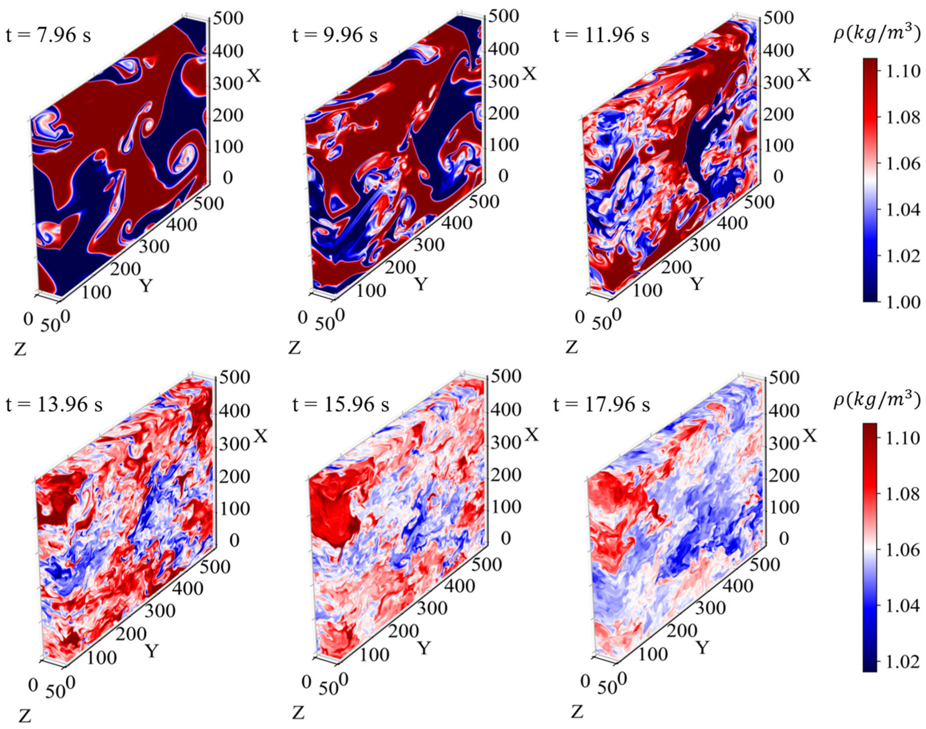
Firstly, we extract 3D density fields from the HBDT dataset at six representative time steps, t = 7.96, 9.96, 11.96, 13.96, 15.96, 17.96 s, with a fixed increment of 2 s between steps. These snapshots were carefully selected to span the most dynamic period of the HBDT simulation. They include the growth phase of turbulent kinetic energy, its peak (around t = 11.4 s), the peak of dissipation rate (around t = 11.56 s), and the subsequent decay of turbulence. As shown in Figure 4, the selected datasets represent the full volumetric density distribution with a spatial resolution of $500\times 500\times 50$, capturing the evolving density structures during mixing. Each 3D density field is then converted to a refractive index field using the Gladstone–Dale relation, as previously described in Section 3.1.2, which serves as input for the subsequent ray tracing simulation.

To ensure the forward simulation realistically mimics experimental BOS conditions, we define a representative set of optical and flow field parameters, as summarized in

Table 1. Optical system parameters for simulating image degradation caused by the HBDT flow field.

Parameters	Value
$f$	105 mm
$l_1+l_2$	1 m
$l_3$	0.1 m
$l_1$	${\displaystyle \frac{1}{5}}\times (l_1+l_2)$

. These include lens focal length $f$, object distances $(l_1+l_2)$, and image distances $(l_3)$, chosen based on typical experimental setups reported in the literature [27]. We position the flow field near the background image; although it may seem counter-intuitive (since increasing the distance between the flow field and the background improves image sharpness), this approach ensures that as much of the background light as possible passes through the flow field and exacerbates distortions caused by the refractive properties of the flow, which provides richer data for phase screen generation. The optical parameters used in our setup are chosen to be representative, not exhaustive. We do not perform a detailed analysis of their individual effects on image formation, as the primary focus of this study is on the accuracy of phase screen reconstruction. A systematic sensitivity analysis of these parameters may be explored in future work dedicated to the optimization of BOS systems.

4.2. Forward and Inverse Simulation

After configuring the optical system and flow field parameters, we proceed with the forward simulation using ray tracing described in Section 3.1. The light rays are traced through the flow field, and the resulting distortions, caused by refractive index variations, are captured in the degraded image. The degraded image is then compared with the background image to extract the displacement vectors, OPD gradients, and phase screen information according to inverse reconstruction in Section 3.2. 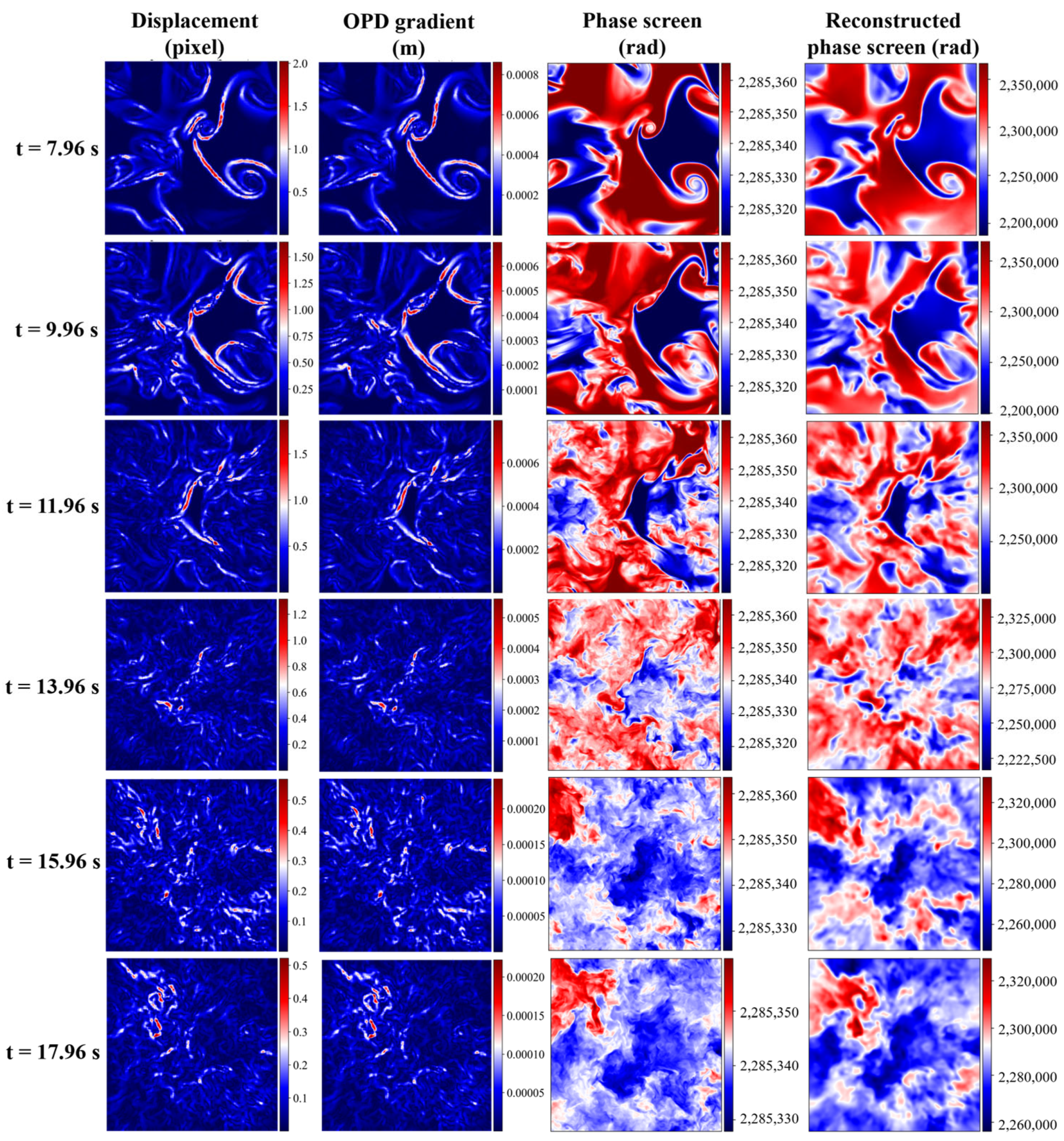Figure 5 presents the simulation and reconstruction results at six different time instances. From top to bottom, the flow field evolves chronologically (7.96 s to 17.96 s), while each column corresponds to a specific type of data: the displacement field, computed from the comparison between the original background image and the degraded image, which reveals the amount of shift in each pixel due to the refractive index variations; the OPD gradients, calculated using the inverse reconstruction method; the original phase screen calculated directly from the 3D density field; the reconstructed phase screen derived from the degraded image using the displacement and gradient data. By qualitatively comparing the two-phase screens, we clearly observe that our reconstructed phase exhibits a high degree of similarity to the original field, and the key flow features, such as vortical structures, are consistently captured by both phase screens.

4.3. Phase Screen Evaluation

After the qualitative assessment, we proceed with a quantitative analysis to further evaluate the accuracy of the reconstructed phase screens. We employ two widely used metrics: relative error (RE) and structural similarity index (SSIM), and they are defined as

$$\begin{array}{c}\mathrm{RE}(x,y)={\displaystyle \frac{\left|{\varphi }_{orig}(x,y)-{\varphi }_{recon}(x,y)\right|}{\left|{\varphi }_{orig}(x,y)\right|}}\times 100\%\\ \mathrm{SSIM}(x,y)={\displaystyle \frac{(2{\mu }_x{\mu }_y+C_1)(2{\sigma }_{xy}+C_2)}{({\mu }_x^2+{\mu }_y^2+C_1)({\sigma }_x^2+{\sigma }_y^2+C_2)}}\end{array}$$

(23)

where ${\mu }_x,{\mu }_y$ are the means of flow fields $x$, $y$, ${\sigma }_x^2,{\sigma }_y^2$ are local variances, and ${\sigma }_{xy}$ is their covariance. The RE provides a measure of the pixel-wise amplitude discrepancy between the original and reconstructed phase screens, while SSIM assesses their structural consistency by considering luminance, contrast, and spatial correlation. These metrics are calculated for all six-time steps to quantitatively assess the reconstruction performance over the entire evolution of the flow field.

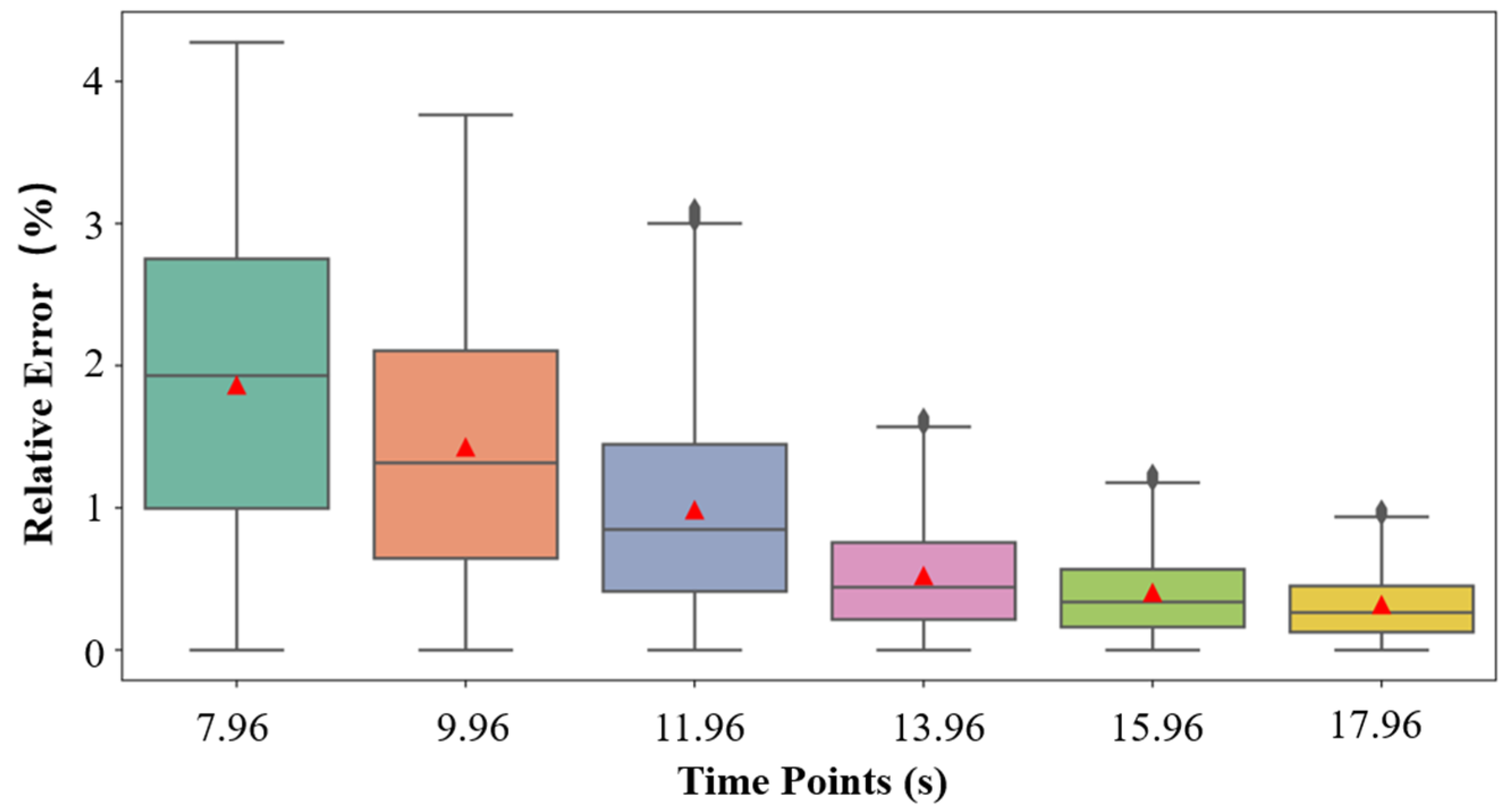
Figure 6 shows the distribution of RE across all pixels between the two-phase screens at different time points. Each box represents the interquartile range (IQR) of the error values, with the central line indicating the median, the boxes covering the middle 50% of the data, and the “whiskers” representing the range of values within 1.5 times the IQR. The red triangle in each box represents the mean error value at that time instance. In Figure 6, we first observe that RE for all time points and all pixels remains below 4%, with the majority even staying under 2%. This indicates that our simulation and reconstruction pipeline maintains a high level of accuracy and robustness across the entire turbulence evolution. More importantly, a clear decreasing trend in both mean and median RE is evident as time progresses. This can be attributed to the physical decay of the turbulent flow. In the early stages (e.g., time steps 7.96 s–11.96 s), the turbulence is strong, and the density field exhibits sharp gradients and complex spatial structures. These features induce stronger optical distortions and larger refractive index fluctuations, which challenge the BOS-based reconstruction and contribute to relatively higher errors and broader distributions. As the simulation progresses (e.g., time steps 13.96 s–17.96 s), the buoyancy-driven turbulence begins to decay, leading to smoother density fields and weaker refractive index gradients. This results in less severe optical distortions, allowing the BOS algorithm to perform more reliably with reduced reconstruction error. Accordingly, the error distributions become narrower, with shorter whiskers and reduced IQRs, indicating improved stability and precision of the reconstruction in weaker turbulence conditions.

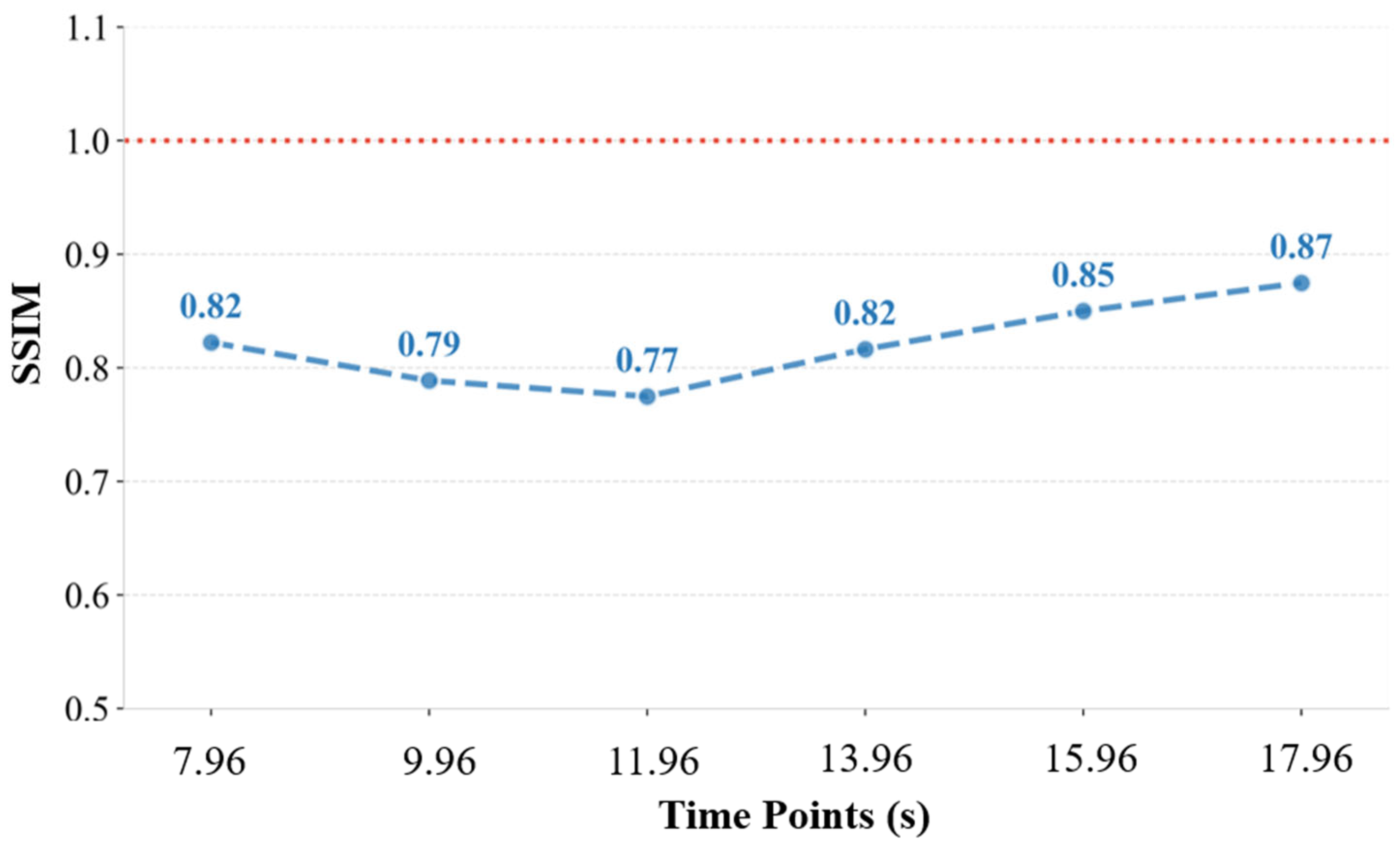
At the same time, in Figure 7, the SSIM values remain above 0.75 across all time points, indicating that our reconstructed flow field preserves the overall structural integrity and spatial patterns of the original field with high fidelity. Interestingly, the SSIM curve exhibits a non-monotonic trend: it decreases initially, reaching a minimum of around 11.96 s, and then gradually increases toward 17.96 s. This variation can be understood by examining the physical evolution of the flow field during the decay of buoyancy-driven turbulence. At the beginning of the selected window (e.g., t = 7.96 s to 11.96 s), although the turbulence is already past its initial development stage, residual large-scale structures and coherent density gradients are still present. These provide strong BOS signals that facilitate accurate reconstruction, contributing to higher SSIM values. In the mid-stage of decay (e.g., t = 11.96 s to 13.96 s), the turbulence enters a more complex transitional regime, where large vortices break down, and small-scale mixing dominates. This stage features increasingly fragmented and fine-grained density structures, which are harder to resolve and reconstruct accurately, leading to a slight drop in SSIM values. As the decay continues further (e.g., t = 15.96 s to 17.96 s), the turbulence weakens significantly, and the flow becomes smoother and more uniform, with lower density gradients. The reduced structural complexity and optical distortion allow the BOS algorithm to recover the flow features more consistently, causing SSIM to rise again. Notably, even during the more challenging mid-decay stage, the SSIM remains above 0.77. This demonstrates the robustness of our reconstruction method in handling varying levels of structural complexity and its effectiveness across different turbulence decay stages.

Through both qualitative comparisons and quantitative metrics across six different time steps, we have demonstrated that phase screens reconstructed from BOS measurements are accurate and stable in the context of turbulent flow fields provided by the JHTDB dataset. Moreover, this capability has a potential application: image restoration. Since the image degradation is caused by phase distortion introduced by the flow field, superimposing the inverse of the reconstructed phase screen onto the original distorted field can mitigate the degradation effects, approximately reverse the distortion, and recover the original image. While this process is not the central focus of the current study, our findings suggest that under suitable conditions, BOS may support not only flow diagnostics but also image correction.

5. Application to Shockwave

Following the successful validation of phase screen reconstruction in the controlled and relatively smooth turbulent fields provided by the JHTDB dataset, we now turn to a more complex and optically challenging scenario—shockwave fields at different Mach numbers. Unlike the continuous refractive index variations in JHTDB, shockwaves introduce sharp discontinuities in pressure, density, and velocity, resulting in highly localized and nonlinear gradients in refractive index. These features produce severe light deflections and wavefront distortions that can significantly compromise the assumptions underlying BOS-based phase reconstruction. In this chapter, we apply the same forward and inverse simulation framework to a series of CFD-generated shockwave fields.

5.1. Flow Field Setup and Simulation

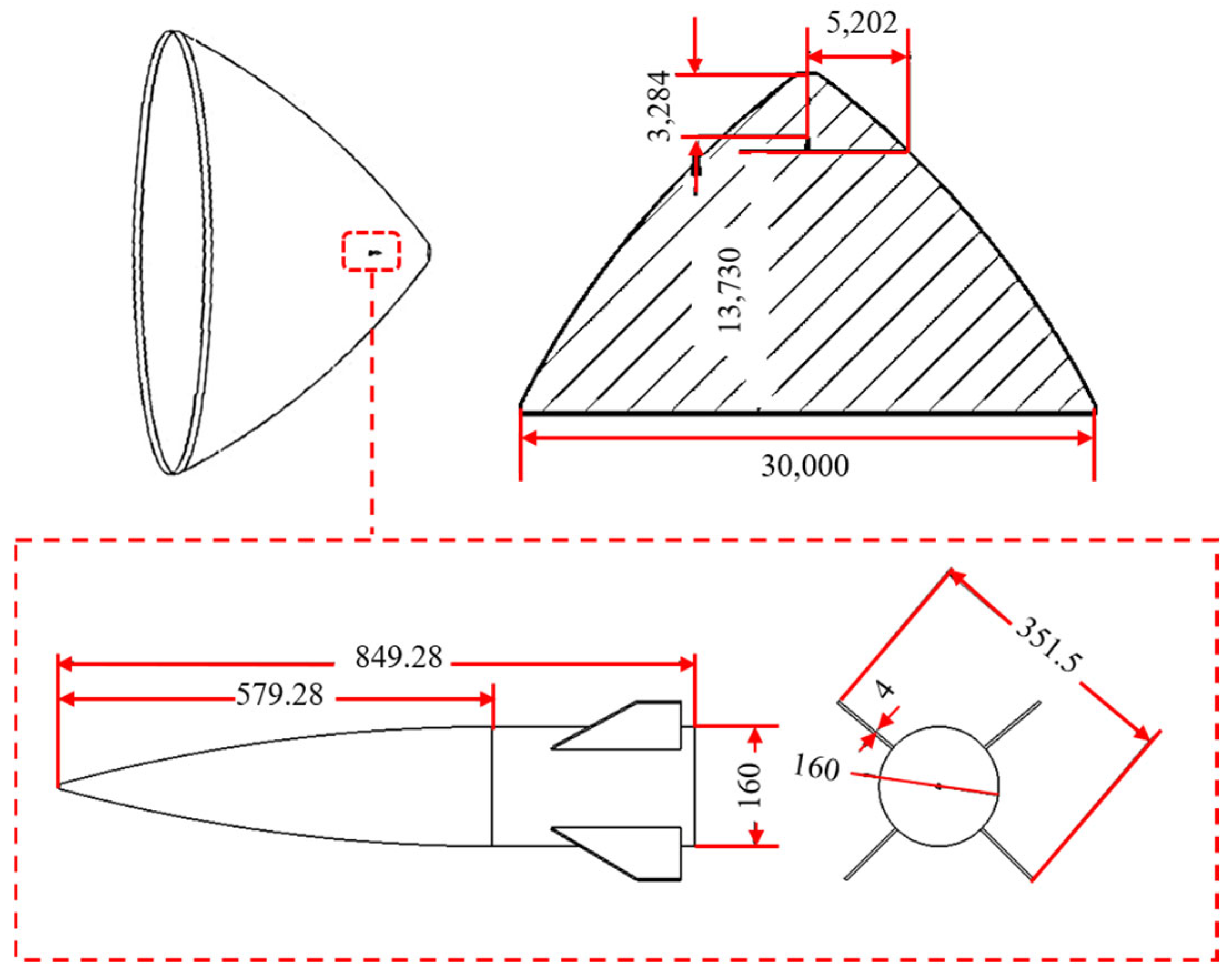
We select a high-speed aircraft model as the analysis object. By defining the computational domain around the aircraft and modeling the external flow field, computational fluid dynamics (CFD) simulations were conducted to obtain the shockwave structures under different Mach numbers. The aircraft model and corresponding flow field setup are illustrated in Figure 8. The parameters of the simulation are shown in

Table 2. Key parameters in the shockwave simulation.

Parameter	Setting
Turbulence Model	$\mathrm{SST} k-\omega$
Target Mach number	3, 4, 5, 6, 7
Solver Type	Density-based
Mesh Type	Hybrid structured-unstructured mesh
Grid Refinement	Refined near shock regions, coarser in low-gradient areas
Convergence Criteria	Residuals < 10−6

.

The resulting density distributions around the aircraft at Mach 3, 4, 5, 6, and 7 clearly exhibit well-defined oblique shock structures, as depicted in Figure 9. As expected, the shockwave forms ahead of the aircraft and extends obliquely downstream. With increasing Mach number, the shock angle becomes steeper, and the shockwave compresses further toward the aircraft’s body. Additionally, the post-shock expansion region grows more pronounced at higher speeds, with density gradually decreasing and the wake becoming more diffuse. These results validate the correctness of the simulated flow fields and provide a solid foundation for analyzing the optical distortions they produce.

5.2. Reconstruction Performance at Short Distances

To directly compare this method with the validation cases in Section 4, we begin by applying the same simulation and reconstruction framework to the shockwave flow fields at relatively short object-to-camera distances. The optical setup, imaging geometry, and BOS parameters are kept identical to those used in Section 4.1. This enables us to evaluate the effectiveness of the phase screen reconstruction method validated in turbulence in transitioning to sharply discontinuous refractive environments.

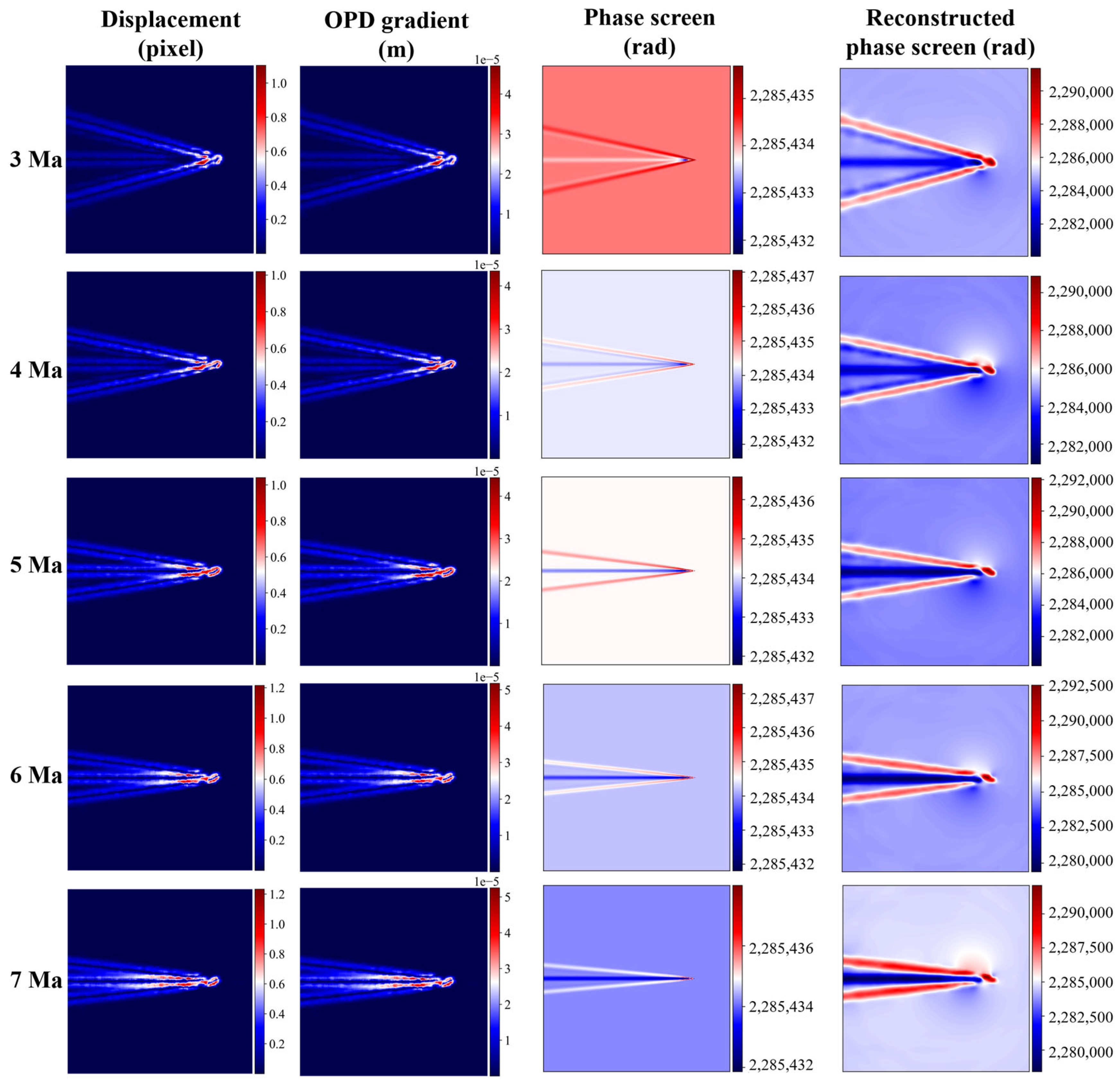
With the generated shockwave fields at different Mach numbers, we proceed with our forward and inverse simulations. The result is shown in Figure 10; each row corresponds to a different Mach number, and from left to right, the columns show the displacement field, the OPD gradient, the original phase screen, and the reconstructed phase screen. Through qualitative observation, we found that the phase screen reconstruction performs well across the evaluated Mach numbers. As the Mach number increases from 3 to 7, the shock structures become progressively sharper and more compressed, and this trend is clearly reflected in both the displacement field and OPD gradient field. Despite the presence of sharp refractive index discontinuities introduced by the shock waves, the reconstructed phase screens generally preserve the global shape and spatial distribution of the phase features. Particularly, the overall geometric shapes of oblique shock waves, such as angular direction, position, and range, are consistently captured.

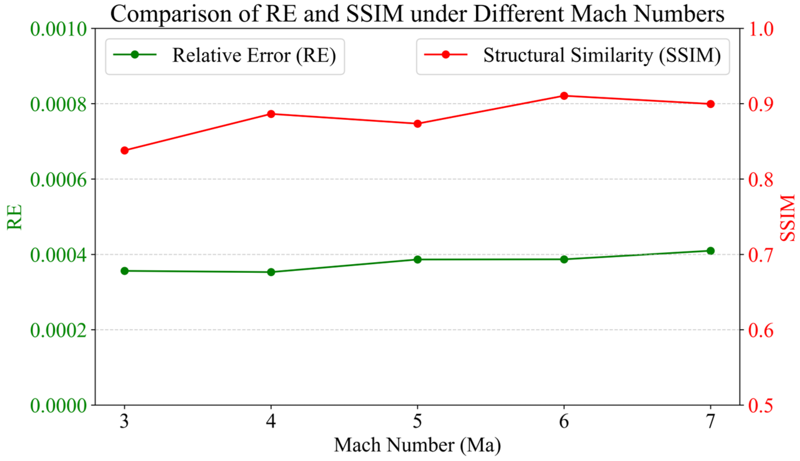
To further evaluate the reconstruction performance, we compute RE and SSIM between the original and reconstructed phase screens across different Mach numbers. As shown in Figure 11, the RE values, indicated by the green curve, remain consistently low across all Mach numbers. A slight increase in RE is observed with higher Mach numbers, indicating that the absolute differences between the reconstructed and original phase screens become larger in sharper, more compressed shockwave fields. This is expected as higher Mach numbers introduce stronger refractive index discontinuities and greater optical complexity. Meanwhile, the SSIM values, represented by the red curve, consistently exceed 0.8, suggesting that the reconstructed phase screens retain strong global structural similarity to the original ones. However, a closer inspection reveals that SSIM does not monotonically increase or decrease with Mach number but, instead, exhibits a nonlinear, M-shaped fluctuation. This trend likely reflects a balance between two competing effects: on the one hand, increasing Mach numbers lead to more distinct and well-defined shock structures, which enhances structural alignment and boosts SSIM; on the other hand, these same high-gradient regions, particularly near the shock tip, are more prone to localized reconstruction errors, which suppress SSIM.

Both RE and SSIM confirm the overall accuracy of the reconstruction, particularly in preserving the global geometry of the shock structures. However, despite these promising results, there are still two noteworthy phenomena in reconstructed phase screens. First, the reconstructed shock boundaries appear wider than those in the original phase screens. This broadening effect may originate from the ray tracing model used in the forward simulation step. When encountering sharp refractive index gradients, rays tend to scatter or overlap, introducing spatial blur in the displacement fields and ultimately smoothing the OPD gradients. Second, and more critically, the shock tip region exhibits a clear reconstruction failure. Although the rest of the shock front was accurately captured, in the reconstructed phase screen, the tip showed offset distortion and a severe trend with increasing Mach number. This deviation is primarily due to the extremely high local gradients at the tip, which lead to rapidly diverging ray paths and severely ill-posed displacement observations. Additionally, the CG algorithm used for phase reconstruction is sensitive to such localized high-gradient zones, where small numerical inaccuracies can accumulate during the iterative process, resulting in visible deviations. These two limitations highlight the inherent challenges in reconstructing phase information in the presence of strong spatial nonlinearities.

5.3. Reconstruction Limitations at Long Distances

While the results in the previous section demonstrate that the phase screen reconstruction method performs reliably at short object-to-camera distances, such conditions are often unrealistic in practical scenarios involving large-scale atmospheric or aerospace applications. In real-world BOS deployments, the optical path between the object (e.g., a supersonic aircraft) and the imaging system often spans tens of kilometers, especially in airborne or ground-based surveillance systems. Under such long-distance propagation, the interaction between the shock-induced refractive index variations and the optical wave becomes significantly more complex. To investigate the robustness of the reconstruction framework under more realistic imaging geometries, we extend our simulation by increasing the object-to-camera distance from the near-field setup in Section 5.2 to practical values. The optical system and flow field parameters used for this simulation are listed in

Table 3. Optical system parameters for simulating image degradation caused by the shock wave field.

Parameters	Value
$f$	800 mm
$l_1+l_2$	10 km/30 km/50 km/70 km
$l_3$	$1/\left({\displaystyle \frac{1}{f}}-{\displaystyle \frac{1}{l_1+l_2}}\right)$
$l_1$	${\displaystyle \frac{1}{10}}\times (l_1+l_2)$

, including four object distances (10 km, 30 km, 50 km, and 70 km) for each Mach number case. In total, 20 combinations are tested to systematically assess how increasing the distance between the object and the imaging system exacerbates optical distortions.

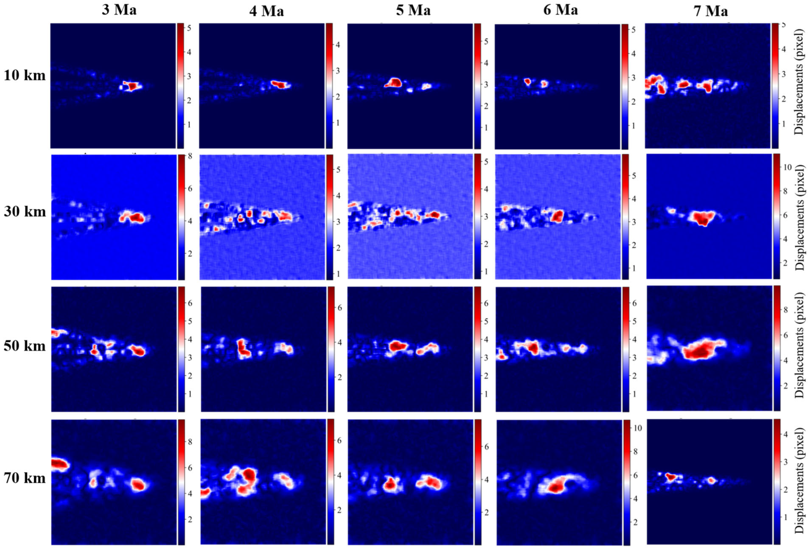
As the light propagates through the shockwave-distorted refractive field, the resulting image distortions become increasingly pronounced with greater object distances and higher Mach numbers. These distortions manifest as significant deflections of light rays, which are effectively captured in the optical flow displacement fields extracted from the simulated degraded images. Figure 12 presents the computed displacement fields across various Mach numbers and object distances. From top to bottom, the rows correspond to increasing object distances of 10 km, 30 km, 50 km, and 70 km, while from left to right, the columns represent Mach numbers (3, 4, 5, 6, and 7). The color maps visualize the magnitude of pixel displacement, highlighting regions of strong deflection associated with the presence of shock waves.

Several clear trends emerge from the results. Firstly, as the Mach number increases, the corresponding shock structures become more intense and compact, generating stronger and more localized refractive gradients. This leads to highly concentrated regions of large displacement in the optical flow maps, particularly near the shock fronts. These patterns become increasingly prominent from Mach 3 to Mach 7, reflecting the growing intensity of the underlying flow field. At Mach 6 and 7, saturation zones emerge in the displacement maps, suggesting that the deflected rays diverge significantly, potentially leaving the imaging plane or overlapping with one another. Simultaneously, increasing the object distance leads to a general amplification of the displacement magnitude across the entire image. This is due to the cumulative nature of refractive effects over long propagation paths: even small angular deflections accumulate into large positional shifts at the imaging plane. Moreover, at longer distances, the displacement fields become noisier and exhibit high-frequency artifacts. These features are not representative of actual flow structures but result from amplified ray path irregularities and numerical sensitivity during ray tracing in highly nonlinear media.

Under remote imaging conditions, as the distance between the object and the camera increases, severe image distortion makes phase screen reconstruction impractical. However, the optical flow field itself still has information, and displacement maps can capture significant features of the impact structure, which lays the foundation for BOS target recognition and feature extraction.

6. Discussion

This study presents a unified numerical framework for image degradation simulation and phase reconstruction. By integrating ray tracing, optical flow estimation, and iterative inverse modeling, this framework provides a virtual platform for evaluating BOS performance under controlled optical and flow conditions. This approach enables not only forward simulation of image distortion but also accurate inverse reconstruction of the flow-induced OPD, offering new insights for both optical diagnostics and image-based flow analysis. We validated the framework using two representative flow fields: a buoyancy-driven turbulence case from the JHTDB and a synthetic compressible shock wave field.

In the JHTDB case, the turbulent flow evolves from peak intensity to a decaying phase with time-dependent refractive index gradients. Our results show that the BOS-based method reconstructs the phase screen with high fidelity across this entire evolution, as the relative error remains below 4%, and the SSIM consistently exceeds 0.75. These results highlight the method’s accuracy and robustness even as turbulence intensity and flow structure gradually diminish. Compared to previous works, which primarily focused on displacement estimation or qualitative visualization [31], our method provides quantitative, pixel-wise recovery of the phase structure, offering strong potential for high-precision image restoration in moderate refractive environments.

In the synthetic shock wave case, we investigated BOS performance across different imaging distances under compressible flow with sharp refractive index discontinuities. Our findings reveal that while near-field conditions allow for partial phase reconstruction, long-range imaging suffers from severe optical degradation, making inverse recovery ill-posed. Nevertheless, even under these degraded conditions, the optical flow field retains interpretable features that correlate with underlying shock structures. This suggests a promising direction for long-range target recognition, particularly in aerospace applications where detecting and tracking flow-induced patterns is more important than reconstructing exact phase values.

Our framework advances BOS from a primarily experimental technique to a simulation-verified, quantitative diagnostic tool. It bridges computational fluid dynamics, geometric optics, and image processing, enabling rigorous, multi-scale evaluation of BOS systems before experimental deployment. However, the current model only considers refractive effects and neglects scattering phenomena caused by aerosols or particulates, which are common in atmospheric conditions. Extending the framework to include radiative transfer or stochastic ray tracing would allow for the simulation of combined refractive and scattering distortions, enabling more comprehensive modeling of real-world degraded imaging, such as foggy or smoky environments. At the same time, future studies could integrate high-resolution CFD simulations or experimental BOS data to test the framework in more realistic or mixed-modal scenarios. This would support applications in wind tunnel diagnostics, hypersonic vehicle design, and atmospheric turbulence compensation.

7. Conclusions

This paper presents a numerical BOS framework capable of simulating and reconstructing flow-induced optical phase distortions. By combining ray tracing, optical flow analysis, and conjugate gradient methods, we enable both forward modeling and inverse recovery of flow field structures. Validation with decaying turbulence from the JHTDB and synthetic shock wave fields demonstrates that the method can accurately reconstruct phase screens under moderate refractive conditions and extract interpretable motion patterns even in highly degraded images. These results confirm the potential of BOS not only for image restoration but also for flow diagnostics and feature recognition in complex optical environments.

References

- Guiomar, F.P.; Fernandes, M.A.; Nascimento, J.L.; Rodrigues, V.; Montetiro, P.P. Coherent free-space optical communications: Opportunities and challenges. J. Light. Technol. 2022, 40, 3173–3186. [Google Scholar] [CrossRef]
- Richter, R. Atmospheric correction methods for optical remote sensing imagery of land. In Advances in Environmental Remote Sensing: Remote Sensing Applications, 1st ed.; Taylor Francis: Abingdon, UK, 2011; pp. 161–172. [Google Scholar]
- Cossu, G.; Ciaramella, E. Optical propagation through atmospheric turbulence for space links. In Proceedings of the IEEE Photonics Global Conference (PGC), Stockholm, Sweden, 21–23 August 2023; pp. 17–22. [Google Scholar]
- Ruizhong, R. Modern Atmospheric Optics; Science Press: Beijing, China, 2012; p. 87. [Google Scholar]
- Galaktionov, I.; Nikitin, A.; Sheldakova, J.; Toporovsky, V.; Kudryashov, A. Focusing of a laser beam passed through a moderately scattering medium using phase-only spatial light modulator. Photonics 2022, 9, 296. [Google Scholar] [CrossRef]
- Giggenbach, D.; Shrestha, A. Atmospheric absorption and scattering impact on optical satellite-ground links. Int. J. Satell. Commun. Netw. 2022, 40, 157–176. [Google Scholar] [CrossRef]
- Hashemipour, S.H.; Ogli, A.S.; Mohammadian, N. The effect of atmosphere disturbances on laser beam propagation. Key Eng. Mater. 2012, 500, 3–8. [Google Scholar]
- Fried, D.L. Optical resolution through a randomly inhomogeneous medium for very long and very short exposures. J. Opt. Soc. Am. 1966, 56, 1372–1379. [Google Scholar] [CrossRef]
- Tatarskii, V.I. The Effects of the Turbulent Atmosphere on Wave Propagation; Israel Program for Scientific Translations: Jerusalem, Israel, 1971. [Google Scholar]
- Andrews, L.C.; Phillips, R.L. Laser Beam Propagation Through Random Media, 2nd ed.; SPIE: Bellingham, WA, USA, 2005. [Google Scholar]
- Banakh, V.A.; Sukharev, A.A.; Falits, A.V. Optical beam distortions induced by a shock wave. Appl. Opt. 2015, 54, 2023–2031. [Google Scholar] [CrossRef] [PubMed]
- Guo, G.; Liu, H.; Zhang, B. Aero-optical effects of an optical seeker with a supersonic jet for hypersonic vehicles in near space. Appl. Opt. 2016, 55, 4741–4751. [Google Scholar] [CrossRef] [PubMed]
- Xie, J.; Bai, L.; Wang, Y.K.; Quiang, L. Influence of refractive index accurate model of supersonic vehicle window flow field on aero-optical characteristics. Optik 2022, 252, 168524. [Google Scholar] [CrossRef]
- Schmidt, J.D. Numerical Simulation of Optical Wave Propagation with Examples in MATLAB; Chapter 10; SPIE: Bellingham, WA, USA, 2010. [Google Scholar]
- Tyson, R.K.; Frazier, B.W. Principles of Adaptive Optics, 5th ed.; CRC Press: Boca Raton, FL, USA, 2022. [Google Scholar]
- Settles, G.S.; Hargather, M.J. A review of recent developments in schlieren and shadowgraph techniques. Meas. Sci. Technol. 2017, 28, 042001. [Google Scholar] [CrossRef]
- Raffel, M. Background-oriented schlieren (BOS) techniques. Exp. Fluids 2015, 56, 60. [Google Scholar] [CrossRef]
- Yuan, X. Recent advances in background oriented Schlieren and its applications. J. Exp. Fluid Mech. 2022, 36, 30–48. [Google Scholar]
- Venkatakrishnan, L.; Meier, G.E.A. Density measurements using the background oriented schlieren technique. Exp. Fluids 2004, 37, 237–247. [Google Scholar] [CrossRef]
- Richard, H.; Raffel, M. Principle and applications of the background oriented schlieren (BOS) method. Meas. Sci. Technol. 2001, 12, 1576. [Google Scholar] [CrossRef]
- Raffel, M.; Tung, C.; Richard, H.; Yu, Y. Background oriented stereoscopic schlieren (BOSS) for full scale helicopter vortex characterization. In Proceedings of the 9th International Symposium on Flow Visualization, Edinburgh, UK, 22–25 August 2000; pp. 23–24. [Google Scholar]
- Heineck, J.T.; Banks, D.; Schairer, E.T.; Haering, E.A., Jr.; Bean, P.S. Background oriented schlieren (BOS) of a supersonic aircraft in flight. In Proceedings of the AIAA Flight Testing Conference, Washington, DC, USA, 13–17 June 2016; p. 3356. [Google Scholar]
- Hill, M.A.; Haering, E.A. Flow visualization of aircraft in flight by means of background oriented schlieren using celestial objects. In Proceedings of the 33rd AIAA Aerodynamic Measurement Technology and Ground Testing Conference, Denver, CO, USA, 5–9 June 2017; p. 3553. [Google Scholar]
- Smith, N.T.; Heineck, J.T.; Schairer, E.T. Optical flow for flight and wind tunnel background oriented schlieren imaging. In Proceedings of the 55th AIAA Aerospace Sciences Meeting, Grapevine, TX, USA, 9–13 January 2017; p. 0472. [Google Scholar]
- Hao-Lin, D.; Shi-He, Y.; Yang-Zhu, Z.; He, L. Experimental investigation on aero-optics of supersonic turbulent boundary layers at different light incident angles. Acta Phys. Sin. 2017, 66, 4201. [Google Scholar] [CrossRef]
- Ding, H.; Yi, S.; Ouyang, T.; Shi, Y.; He, L. Influence of turbulence structure with different scale on aero-optics induced by supersonic turbulent boundary layer. Optik 2020, 202, 163565. [Google Scholar] [CrossRef]
- Rajendran, L.K.; Bane., S.P.M.; Vlachos, P.P. PIV/BOS synthetic image generation in variable density environments for error analysis and experiment design. Meas. Sci. Technol. 2019, 30, 085302. [Google Scholar] [CrossRef]
- Farnebäck, G. Two-frame motion estimation based on polynomial expansion. In Image Analysis: 13th Scandinavian Conference, SCIA 2003, Halmstad, Sweden, 29 June–2 July 2003 Proceedings; Bigun, J., Gustavsson, T., Eds.; Springer: Berlin/Heidelberg, Germany, 2003; Volume 2749, pp. 363–370. [Google Scholar]
- Liu, S.; Mei, H.; Ren, Y.; Tao, Z.; Abdukirim, A.; Zhang, J.; Li, Y.; Rao, R. Research on flow field detection system with high precision based on background oriented schlieren. Acta Photonica Sin. 2022, 51, 1112002. [Google Scholar]
- Livescu, D.; Canada, C.; Kanov, K.; Burns, R.; Pulido, J. Homogeneous Buoyancy Driven Turbulence Data Set; National Science Foundation: Alexandria, VA, USA, 2014.
- Akatsuka, J.; Nagai, S. Flow visualization by a simplified BOS technique. In Proceedings of the 29th AIAA Applied Aerodynamics Conference, Honolulu, HI, USA, 27–30 June 2011; p. 3653. [Google Scholar]
Figure 1.
Sketch of BOS imaging configuration. The yellow line indicates the original, undeflected light path, while the solid green line illustrates the actual path being refracted through the turbulent flow field. The dashed green line represents the centerline of the refracted ray. As the ray passes through the medium, it is bent by a total deflection angle , which causes the image of the background point to shift by a displacement on the sensor. The angles and describe the trajectory of the ray as it enters and exits the flow region. is the distance from the background plane to the center of the flow field; is the distance from the center of the flow field to the lens, and is the distance from the CCD to the lens.
Figure 2.
Schematic diagram of simulation design process.
Figure 3.
High contrast background image in BOS system.
Figure 4.
The 3D density distributions from the HBDT flow field at six time steps from t = 7.96 s to t = 17.96 s, showing the temporal evolution of turbulence. The axes X, Y, and Z represent the spatial resolution of the data.
Figure 5.
BOS-based reconstruction results for the JHTDB flow field at six different time steps (7.96 s to 11.96 s). From top to bottom: time evolution of the flow. From left to right: displacement field, OPD gradient field, original phase screen (via direct integration), and reconstructed phase screen (via BOS inversion).
Figure 6.
Statistical summary of relative errors between original and reconstructed phase screens.
Figure 7.
SSIM of original and reconstructed phase screens at different time points.
Figure 8.
The aircraft model and corresponding flow field setup (Unit: mm).
Figure 9.
Density distribution of the shock wave field at different Mach numbers.
Figure 10.
BOS-based reconstruction results for the shockwave at different Mach numbers (3 Ma to 7 Ma). From top to bottom: gradually increasing Mach number. From left to right: displacement field, OPD gradient field, original phase screen (via direct integration), and reconstructed phase screen (via BOS inversion).
Figure 11.
Comparison of RE and SSIM between original and reconstructed phase screens across different Mach numbers.
Figure 12.
Optical flow displacement fields computed from degraded images under varying shockwave conditions. Columns correspond to Mach numbers 3–7 (top to bottom), and rows represent object distances of 10 km, 30 km, 50 km, and 70 km (left to right). Color intensity encodes displacement magnitude, highlighting regions of strong optical deflection induced by shockwave structures.