Review

Some Insights on Kerr Lensing Effects

by
Kamel Aït-Ameur
1,* and
Abdelkrim Hasnaoui
2
1
Centre de Recherche sur les Ions, les Matériaux et la Photonique (CIMAP), UMR6252 CEA-CNRS-ENSICAEN-Université de Caen, 6 Bd Maréchal Juin, CEDEX 4, F14050 Caen, France
2
Institut National d’Optométrie d’Ouled Fayet (INOOF), Residence les Palmiers, Ouled Fayet, Algiers RW233, Algeria
*
Author to whom correspondence should be addressed.
Photonics 2025, 12(6), 596; https://doi.org/10.3390/photonics12060596
Submission received: 8 May 2025 / Revised: 5 June 2025 / Accepted: 7 June 2025 / Published: 10 June 2025

Abstract

The research on high-order transverse modes in lasers was largely abandoned a few years after the invention of the laser in 1960. The main reason for this was that high-order beams are more divergent and less bright than the Gaussian beam. In the present paper, we showed that the behaviour of L G p 0 beams faced to the optical Kerr effect (OKE) varies considerably depending on the mode order (p = 0 or p 1 ). We focused our attention on the properties of L G 00 and L G 10 beams when subject to OKE, and we found that the L G 10 beam keeps its focusability much better than the L G 00 beam. This property has at least two applications concerning first the conception of high-intensity laser chains not based on a Gaussian beam but on an L G 10 beam and second, the use of an L G 10 beam instead of the usual Gaussian beam which can reduce drastically the protection of optical limiters based on OKE; this constitutes a counter-measure against such limiters.

1. Introduction

Before becoming involved in the issue itself, we should start by recalling the optical Kerr effect (OKE) taking place in a transparent dielectric illuminated by a laser beam characterised by its intensity profile I ( ρ ) , where ρ is the radial coordinate. The OKE is a nonlinear mechanism causing an intensity-dependent change in the refractive index profile n ( ρ ) of the material given by the following:
n ( ρ ) = n 1 + n 2 I ( ρ )
where n 1 ( n 2 ) is the usual (nonlinear) refractive index. The nonlinear refractive index can be positive or negative, but subsequently it will be assumed positive as for most of the nonlinear materials. The studies on light propagation in Kerr medium began intensively after the invention of the first laser in 1960, according to their capacity to generate the highest optical intensity. At that time, the major concern was related to the self-focusing phenomenon having deleterious effects, such as filamentation and beam breakup, with regard to the amplification of high-power laser pulses [1,2]. These aspects of nonlinear propagation inside a Kerr medium are ignored in this paper. We instead focus on the effect of a thin Kerr medium taking the form of a slice of nonlinear material having a thickness d as shown in Figure 1. The latter involves an incident Gaussian beam, which could also be a high-order L G p 0 radial Laguerre–Gauss beam considered later, incident on a Kerr medium of thickness d set against a focusing lens of focal length f L . This self-action of the laser beam leads to a shift towards the lens of the best focus, i.e., the axis point where the intensity is maximum. To this focal shift is associated a Kerr lensing effect which is not pure since it contains high-order spherical aberrations. The modelling of the Kerr lensing effect is fundamental in many applications of the Kerr lensing effect, such as the peculiar regime of laser oscillation usually called as Kerr-lens-mode-locking (KLM) [3,4,5,6]. The modelling of the Kerr lens induced by a Gaussian beam seemed resolved after the 1960s through the well-known parabolic approximation. In Section 2, we revisit this modelling by using a Zernike polynomial decomposition, and give a new expression for the Kerr focal length characterising a thin slice of Kerr medium illuminated by a Gaussian beam or a L G p 0 beam (one peak surrounded by p rings).
The nonlinear phase shift induced in the Kerr medium causes a distortion of the emerging beam changing its M 2 and intensity profile in the plane z = f L , i.e., the geometrical focal plane of the focusing lens. It is well known that when the incident beam is Gaussian, the resulting Kerr aberration has tended to reduce the focused intensity in the plane z = f L . In Section 3, it is shown that this is not the case when the incident beam is a high-order L G p 0 beam, and that it could have very important practical consequences in high-intensity pulses amplifications and in the protective capacity of optical limiters based on the OKE.
The numerous publications on the Kerr effect were conducted in the 1970s and 1980s. They are essentially devoted to the problematic of small- and large-scale self-focusing occurring in high-intensity laser chains. In the 1990s, the research on OKE was mostly focused on Kerr lens mode-locking (KLM) of lasers for generating ultrashort laser pulses. It seems that the studies on the Kerr effect will not be exhausted soon, as they are currently oriented to other fields of physics such as cold atoms [7], vacuum [8], gravitational waves [9], and black holes [10].

2. Kerr Lensing Effect (KLE)

Focusing a laser beam subject to aberrations is a major area of concern which has been applied to spherical aberrations [11,12,13,14,15,16,17,18,19] and to OKE [20,21,22,23,24,25,26,27,28,29]. In this section, we discuss the focal length associated with the self-induced Kerr lens enabling an explanation for the focal shift of the best focus. The other phenomena induced by the OKE, such as beam reshaping, are considered in other sections. An adequate modelling of the Kerr lensing effect is of primary importance when modelling analytically the so-called nonlinear losses hitting a laser beam and crossing a Kerr medium and a diaphragm. This latter point is of key importance when analytically simulating l topics such as Kerr lens mode locking, optical limiters, and Z-scan technique.

2.1. Kerr Lens Effect Induced by a Gaussian Beam

The incident beam on the Kerr medium of thickness d is a collimated radial Laguerre–Gauss L G p 0 beam having an electric field E i n ( ρ ) given as follows:
E i n ( ρ ) = E 0 × L p ( 2 ρ 2 / W 2 ) × exp [ ρ 2 / W 2 ]
where W = 1 mm is the width of the Gaussian term in Equation (1) corresponding to the width of the L G 00 beam, i.e., the Gaussian beam. The nonlinear phase shift profile Δ ϕ ( ρ ) induced by the Kerr effect takes the following form:
Δ ϕ ( ρ ) = k n 2 I ( ρ )
where k = 2 π / λ , with the wavelength λ = 1064 nm, and I ( ρ ) = ( E i n ( ρ ) 2 . As related in the Section 1, the Kerr medium of thickness d is assumed to be thin. This means that the analysis of the self-focusing effect occurs outside the Kerr medium through linear propagation in free space. For that, we need the knowledge of the electric field E d ( r , z ) resulting from the diffraction of the electric field distribution E i n ( ρ ) passing through the nonlinear phase shift profile Δ φ ( ρ ) . The diffracted electric field E d ( r , z ) is handled by the usual Fresnel–Kirchhoff integral given by the following:
E d ( r , z ) = 2 π λ z 0 E i n ( ρ ) exp [ i Δ ϕ ( ρ , t ) ] × exp i π ρ 2 λ 1 f L 1 z J 0 2 π λ L r . ρ ρ d ρ
where r is the radial coordinate in plane z, and J 0 is the zero-order Bessel function of first order. The Fresnel–Kirchhoff diffraction integral allows the determination of the transverse distribution of the diffracted field E d in any plane z. The diffraction integral given above is calculated numerically by using a FORTRAN routine based on the numerical integrator dqdag from the International Mathematics and Statistical Library (IMSL). In the following, all the intensity distributions are given in arbitrary units but remain comparable.
Before concentrating on the effect of self-focusing deduced from the spatial distribution of the diffracted intensity I d ( r , z ) = E d ( r , z ) 2 , we recall briefly the basis of the classical concept of the Kerr lens theory known as parabolic approximation, which has been widely used since the 1960s in the case of an incident Gaussian beam having the following transverse intensity profile:
I ( ρ ) = I 0 exp [ 2 ρ 2 / W 2 ]
The phase aberration profile (PAP) Δ ϕ ( ρ ) induced by the Kerr effect can then be written as follows:
Δ ϕ ( ρ ) = ϕ 0 exp [ 2 ρ 2 / W 2 ]
where ϕ 0 the on-axis phase shift is given by
ϕ 0 = 4 n 2 P d λ W 2
with P = ( π W 2 I 0 / 2 ) the incident beam power. It is important to note that the nonlinear phase shift Δ ϕ ( ρ ) given in Equation (5) has to be considered as a phase aberration containing a focusing term and high order spherical aberrations (see Appendix A). The well-known parabolic approximation consists of developing at first order the exponential term in Equation (5):
Δ ϕ ( ρ ) ϕ 0 1 2 ρ 2 W 2
Note that the phase shift profile given in Equation (7) is quadratic, and consequently by definition corresponds to a pure distributed lens (without aberration) which can be characterised by an equivalent focal length f proposed by Kogelnik [28]:
f = π W 2 2 λ ϕ 0
Consequently, the longitudinal position z max after the focusing lens of the best focus should be given by the following:
1 z max = 1 f L + 1 f
It is interesting to compare z max with the position z max of the best focus deduced from the maximum of intensity I d , calculated using the diffraction integral given in Equation (3). The comparison of the relative variations in ( z max f L ) / f L and ( z max f L ) / f L versus the on-axis nonlinear phase shift ϕ 0 are shown in Figure 2. It should be recognised that the parabolic approximation is unable to explain the variations of ( z max f L ) / f L . At higher values of ϕ 0 the discrepancy between z max and z max becomes increasingly important. Note that high values for ϕ 0 can be easily obtained for a particular family of nonlinear materials (plasmonic structures, metamaterials) having a large nonlinear response, i.e., large or huge n 2 [29,30,31,32].
Since the Kerr effect behaves as a lensing effect, it is important that the Kerr lensing effect should be modelled as best as possible in order to give an account of the best focus position, i.e., the position z max . For that, we determine the “mean focal length” (MFL), associated with the PAP given by Equation (5), and defined by C. Mafusire and A. Forbes [33]. The MFL determination, given in Appendix A, is founded on the decomposition of the PAP on the basis of Zernike polynomials. There are four possibilities to define an MFL associated with the Gaussian PAP (Equation (5)) since there is a quadratic term in the four Zernike polynomials of interest (defocus, primary spherical aberration (SA), secondary SA, tertiary SA). In the following, these four possible mean focal lengths are noted ( f 1 ,   f 2 ,   f 3 ,   f 4 ) and determined for a Gaussian illumination (Equation (A3)). The next step is to determine the MFL from ( f 1 ,   f 2 ,   f 3 ,   f 4 ) which is closest to the Kerr focal length f K , deduced from the through position of the best focus z max , determined by using the following diffraction integral:
1 f K = 1 z max 1 f L
Equations (A7)–(A10) show that any MFL among ( f 1 ,   f 2 ,   f 3 ,   f 4 ) can be written as
f j = K j W 2 λ ϕ 0
with K 1 = 7.4 ; K 2 = 1.65 ; K 3 = 0.71 ; and K 4 = 0.44 . In Equation (11), f j , W and λ are expressed in millimetres. Note that the mean focal length (MFL) obtained in the framework of Zernike modelling looks like Equation (8) except for the factor multiplying the ratio W 2 / ( λ ϕ 0 ) . Before comparing the four focal lengths ( f 1 ,   f 2 ,   f 3 ,   f 4 ) to f K which can be considered as the “true” Kerr focal length, it is important to check that f K deduced from Equation (10) is effectively proportional to W 2 , and inversely proportional to ϕ 0 . The proportionality between f K and W 2 is effectively confirmed by the plot shown in Figure 3. Figure 4 displays the variations of f K which are not fully proportional to 1 / ϕ 0 . The plot in red colour shown in Figure 4 corresponds to a linear fit performed by the soft ORIGIN 6.0 according to the following parameters:
f K = A + B / ϕ 0
with A = −1213 and B = 13,864
where ϕ 0 is in radians. The comparison of Equations (11) and (12) allows the estimation of the constant K, so that the Kerr focal length can be approximated by the following equation:
f K K W 2 λ ϕ 0   with K = 14.7
where f K , λ, and W are expressed in millimetres.
For the sake of completeness, we need to compare the four MFLs ( f 1 ,   f 2 ,   f 3 ,   f 4 ) with f K as shown in Figure 5. The conclusion is that none of the focal lengths ( f 1 ,   f 2 ,   f 3 ,   f 4 ) is appropriate for modelling the Kerr focal length f K . However, the analysis of the Kerr focusing effect using the Zernike polynomial formalism enables confirmation of the scale low given by Equation (8) but with a constant K = 14.7 instead of K = 1.57 provided by the usual parabolic approximation.
In an article published a few years ago [34], six possible focal lengths characterising the Kerr lensing effect were identified. Here, we propose a seventh way for defining the focal length of the KLE by considering the variations of the on-axis intensity in the focal plane z = f L of the focusing lens, calculated by using Equation (3), shown in Figure 6.
For modelling analytically the variations of I d ( 0 , z = f L ) versus ϕ 0 we assume that the beam emerging from the ensemble (Kerr medium+ focusing lens) remains Gaussian while knowing that it is not the case, as is seen later. In addition, we assume that the KLE is characterised by a pure lens of focal length f K expressed by Equation (13). The objective is the determination of the constant K from the plot in Figure 6. The KLE is symbolised in Figure 7 showing the focal shift of the Gaussian beam (plane P′) toward the focusing lens.
The collimated Gaussian beam (GB) of width W is focused by the lens of focal length noted f 0 and given as follows:
1 f 0 = 1 f K + 1 f L
In the absence of OKE, the GB of power P G focuses in plane P and is characterised by an on-axis intensity I 0 and a beam-waist width W 0 given below:
W 0 = λ f L π W   and   I 0 = 2 π W 2 P G λ 2 f L 2
When the OKE operates, the GB focuses in plane P′ and is characterised by an on-axis intensity noted I 0 and a beam-waist width W 0 given as follows:
W 0 = λ f 0 π W   and   I 0 = 2 π W 2 P G λ 2 1 f L + 1 f K 2
The on-axis intensity in plane P is the on-axis intensity of the GB having travelled the distance ( f L f 0 ) from the plane P′, and is given as below:
I ( 0 , f L f 0 ) = I 0 1 + f L f 0 z R 2
With   z R = π ( W 0 ) 2 λ
The next step is to consider the case where the denominator in Equation (17) can be reduced to [ ( f L f 0 ) / z R ] 2 when ϕ 0 is sufficiently large. To find the minimum value of ϕ 0 over which the approximation that we have just described is valid, we need to estimate the Rayleigh distance z R which is smaller than z R and is equal to 0.84 mm. It is important to note that f 0 is equal to z max as given in Figure 2. Consequently, the value of ϕ 0 for which the ratio [ ( f L f 0 ) / z R ] 2 is equal to 10 (arbitrary criterion) corresponds to a ratio ( z max f L ) / f L equal to about −5%. As a result, the denominator in Equation (17) can be reduced to [ ( f L f 0 ) / z R ] 2 if ϕ 0 6 rad. After some simple calculations, we obtain the following relation between f K and the on-axis intensity in plane P:
I ( 0 , f L f 0 ) = λ 2 I 0 f K 2 π 2 W 4
From Figure 6, we deduce the value of I 0 , which corresponds to the value of I [ 0 , ( f L f 0 ) ] for ϕ 0 = 0 , that is I0 = 3513 a.u. Finally, we obtain the expression of f K as a function of the normalised intensity I [ 0 , ( f L f 0 ) ] / I 0 :
f K = π W 2 λ I [ 0 , ( f L f 0 ) ] I 0
Note that the factor multiplying the square root in Equation (20) is the Rayleigh distance of the incident collimated GB, which is equal to 2952 mm. The variations of f K determined from Equations (10) and (20) are plotted in Figure 8.
A close look at Figure 8 clearly shows that the value of f K determined by using Equation (20) is very close to that obtained by using Equation (10) but for ϕ 0 7 rad which is our starting assumption. Consequently, we can conclude that this seventh method proposed for determining f K from the variations of I d ( 0 , z = f L ) works well. However, it must be said that the agreement is not perfect, and the main source of this disagreement is the hypothesis concerning the Gaussian nature of the beam emerging from the Kerr medium. Indeed, the Gaussian phase shift acts like a beam reshaper, changing the transverse and longitudinal intensity distributions. Indeed, a close look at Figure 9, showing the on-axis intensity distribution for several values of ϕ 0 the nonlinear phase shift, indicates clearly that the Kerr lensing effect is far from being a pure lensing effect in view of the deformation of the on-axis intensity distribution. For confirmation of that, we can also observe in Figure 10 the distortion of the transverse intensity distribution in the plane z = f L for several values of ϕ 0 , which is no longer Gaussian in shape.
Lastly, the most suitable quantity able to quantify how much the distortion of the laser beam emerging from the Kerr medium is important or not, should be to consider its M 2 factor. This parameter is important for characterising the propagation of the beam subject to OKE and is used in the next sections. An M 2 factor close or equal to unity indicates a Gaussian beam while an M 2 factor greater than one indicates a non-Gaussian beam.
The first step for evaluating the M 2 factor of the Gaussian beam diffracted on the Kerr phase shift profile Δ ϕ ( ρ ) is to determine, for several values of ϕ 0 , the longitudinal evolution of the diffracted beam width noted W D . The latter is the beam width based on the second-order intensity moment [35], and is defined as follows:
W D 2 ( z ) = 2 0 I d ( r , z ) r 3 d r 0 I d ( r , z ) r d r
The calculation of W D ( z ) was carried out for 60 values of coordinate z, the distance counted from the combination (Kerr lens + focusing lens) as shown in Figure 1. The longitudinal distribution of W D is characterised by the two following quantities:
(i)
the minimum value of W D , denoted W D min
(ii)
the longitudinal position, denoted z min , where the diffracted beam has a shrinkage which is maximum, i.e., W D = W D min .
Note that z min is not necessarily equal to z max due to the beam distortion. The M 2 factor is then deduced from a fit of the plot W D versus z with the parabola given by Equation (22):
W D 2 ( z ) = W D min 1 + M 2 λ ( z z min ) π W D min 2
The M 2 factor variations of the beam emerging from the Kerr medium versus the nonlinear on-axis phase shift are plotted in Figure 11. As ϕ 0 is increased, the M 2 factor grows, and this confirms that the diffracted beam does not remain Gaussian. The plot in Figure 11 could be roughly approximated by a linear function, but the following more accurate fit is preferred:
M 2 = A + C 1 ϕ 0 + C 2 ϕ 0 2 + C 3 ϕ 0 3 + C 4 ϕ 0 4 + C 5 ϕ 0 5
with A = 1.04, C 1 = 0.0510 , C 2 = 0.0663 , C 3 = 5.018 × 10 3 , C 4 = 1.54 × 10 4 , C 5 = 1.56 × 10 6 . Note that the coefficients A, C 1 , C 2 , … appearing in Equation (23) do not depend on W the incident Gaussian beam width. The M 2 factor of the beam emerging from the Kerr medium depends only on the phase shift ϕ 0 for a given wavelength.

2.2. Kerr Lens Effect Induced by a LGp0 Beam

The radial Laguerre–Gauss beams L G p 0 are characterised by an electric field given by Equation (1), and their transverse intensity profiles, given in Figure 12, are made up of a central peak surrounded by p rings.
Three fundamental quantities characterising the LGp0 beams are the Rayleigh range z R , the beam propagation factor M p 2 , and the longitudinal distribution W p ( z ) of the beam width based on the second-order intensity moment [35]:
z R = π W 0 2 λ M p 2
M p 2 = ( 2 p + 1 )
W p 2 ( z ) = W 0 2 1 + λ M p 2 z π W 0 2 2
where the origin z = 0 of the longitudinal coordinate is in the beam-waist plane of the focused beam, characterised by W 0 the beam-waist radius of the L G 00 beam. It is important to note that the beam width W appearing in Equation (1) has a simple physical meaning only for the fundamental mode L G 00 , i.e., the width of the Gaussian beam. The beam spreading increases with mode order p so that the beam width W p in the far-field ( z > > z R ) is given as follows:
W p = W 2 p + 1
The two quantities allowing illustration of the Kerr lensing effect (KLE) are the relative focal shift ( z max f L ) / f L and the on axis intensity I d ( 0 , z = f L ) which are, respectively, shown in Figure 13 and Figure 14. We cannot strictly speaking describe the plots, for p 1 , in Figure 14 as a focal zoom due to OKE, since the value of ( z max f L ) / f L is less than one percent. It is as if the L G p 0 beams for p 1 are insensitive to the Kerr effect or more precisely are much less sensitive than the usual Gaussian beam. This important property is confirmed by the plot in Figure 13 which shows that the on-axis intensity in plane z = f L remains high even for large values of ϕ 0 , and even greater than the focused intensity obtained for a Gaussian beam. This important feature is very similar to the relative insensitivity of high-order L G p 0 beams subject to a spherical aberration [36,37], and finds, as mentioned later, a promising application to optical limiters and amplification of pulses of high intensity.

3. LGp0 Beams Subject to OKE: Applications

The optical Kerr effect described by Equation (5) must be classified in the category of the phase aberrations whose first effect is to reduce the focused intensity in the plane z = f L when the incident beam on the setup shown in Figure 1 is Gaussian (p = 0). For reference purposes, we recollect that the most common aberration, i.e., the spherical aberration, mainly causes a longitudinal displacement of the best focus position leading to an undesirable reduction in intensity at focal plane z = f L [13,38]. Unsurprisingly, the same behaviour is observed when focusing a Gaussian beam subject to OKE, as shown in Figure 13 for p = 0. Note that the focal shift for p = 0, shown in Figure 14, increases strongly with the nonlinear phase shift ϕ 0 , whereas it is very low for p 1 . That explains why the on-axis intensity in plane z = f L , as shown in Figure 13, remains for p 1 high, even for large ϕ 0 . It should be noted that a similar behaviour has been observed for a “rectified” high-order L G p 0 beam, for p 1 , subject to spherical aberration [36,37]. This capacity to maintain a high on-axis intensity in the focal plane z = f L when focusing a high-order L G p 0 beam subject to optical Kerr effect allows us to envisage at least two important applications which are described below.

3.1. Improving the Focusing Properties of a Laser Beam Subject to OKE

The propagation of ultrafast laser pulses through various optical devices (laser crystal, windows, lenses, prisms) can suffer the consequences of OKE cumulated by this crossing of the diverse materials. To get a clearer picture, let us consider the propagation of a Gaussian laser pulse (700 fs, 220 µJ) having a width W = 1 mm, through a 4 cm fused-silica sample. The resulting on-axis nonlinear phase shift ϕ 0 induced by OKE is about 6 rad [39]. Before going further, it seems useful to define a certain vocabulary used by the community of high-power pulsed lasers which is concerned by the consequences of the optical Kerr effect.
The breakup integral: The “breakup integral” also called “B-integral” [27,28,40,41,42,43] is defined as follows:
B = 2 π n 2 λ 0 d I ( z ) d z
where d is the propagation distance in the Kerr medium characterised by the nonlinear refractive index n 2 , I ( z ) is the laser beam on-axis intensity, λ is the laser wavelength. In the case of a transparent thin Kerr medium, the breakup integral reduces to
B = k n 2 I d
which corresponds to the on-axis phase shift ϕ 0 , previously introduced in Equation (2), namely, B = ϕ 0 . For a long time, the higher values of ϕ 0 were achieved with the few large fusion laser systems involving laser pulses having a duration ranging from some hundred picosesonds to some nanoseconds. These laser systems have very large dimensions such as the lasers developed for instance at the Lawrence Livermore Laboratory in the USA [27,28,42,43,44]. Usually, the nonlinear propagation problem is separated into two parts:
(i)
Small-scale self-focusing: The “small-scale self-focusing” is a phenomenon leading to an exponential growth [27] of spatial irregularities present in the laser pulse which can result in a beam breakup (self-focusing filamentation), i.e., very hot spots in the section of the laser beam. These hot spots, in extreme cases, can destroy the amplifying medium, and must be suppressed using spatial filters [45]. No more attention is given in this paper to small-scale self-focusing.
(ii)
Large-scale self-focusing: The “large-scale self-focusing” is linked directly to the Kerr lensing effect having the tendency to focus the laser pulse more and more as it propagates inside the amplifying medium. In the extreme case, the large scale self-focusing leads to a collapse of the laser beam inside the amplifying medium, thus leading to its damage. It is then important to limit the length of the amplifying medium in order that the beam collapse will never occur. With no further detail, we can expect from the plots in Figure 14 that the amplification of a L G p 0 beam instead of the usual Gaussian beam could be envisaged with a long amplifying medium.
The beam focusability: The laser beam focusability needs to be understood as the ability to achieve a small focus diameter, i.e., a high focused intensity. The beam focusability is a metric largely used in the community of high power lasers but unfortunately is not well defined since it is based on several definitions: power in the bucket [46], beam parameter product [47], Strehl ratio [48]. Each focusability metric has its advantages and disadvantages, well described in [49], and we would, however, prefer to use the Strehl ratio defined as follows:
S = I d ( 0 , z = f L ) ϕ 0 I d ( 0 , z = f L ) ϕ = 0
The variations of the Strehl ratio versus ϕ 0 are shown in Figure 15 for p = 0 to 3. It is important to note the peculiarity of the L G p 0 beams which for ϕ 0 = 0 produce the same on-axis intensity in plane z = f L for a given power, and for whatever the value of the mode order p. As expected, it can be seen that the Strehl ratio decreases quickly with the increase of the nonlinear phase shift ϕ 0 , which is consistent with the usual effect of a phase aberration upon the focusing of a Gaussian beam (p = 0). However, the situation is very different for p 1 since the Strehl ratio remains high, even larger than one, for large values of ϕ 0 . This behaviour can be assimilated as a sort of immunity of L G p 0 beams with p 1 for the optical Kerr effect. In summary, the plots in Figure 15 allow stating that the diffraction of a L G 00 ( L G p 0 with p 1 ) on a Kerr aberration produces a transfer of energy from the beam centre (beam wings) to the wings (beam centre). The values of S larger than unity for p 1 are due to a transfer of energy from the outer rings to the central peak, very similar to the action of a rectification on an L G p 0 beam [50]. At first sight, we may be tempted to think that such a behaviour is unusual. In fact, a similar effect was observed with a spherical aberration [36,37].
The focal zoom: Since the intensity of the laser pulses is obviously time dependent, light will focus at different locations, and as a consequence the best focus will “zoom”, giving rise to the so-called “focal zoom” which is well described in [51]. This effect of focal zoom has a consequence to change the temporal evolution of the focused pulse, i.e., to create a dip in the on-axis intensity in plane z = f L near the moment when the input pulse on the focusing lens reaches its maximum. Note that from the above, the distortion due to OKE has a spatiotemporal nature, which is difficult to be highlighted using a traditional instrument like a CCD camera which usually carries out the transverse intensity profiles because of the “pulse stacking effect”. The latter superposes the fast time evolution of the distorted intensity profile, thereby blurring the temporal distortion noted above. To record experimentally the spatiotemporal distortion of the focused intensity, one has to use a very expensive instrument called a streak camera [43,52].
For improving the focusing of a laser beam subject to OKE, we should pay attention to the L G 10 beam as a candidate to replace the usual Gaussian beam. To be convinced of this choice, let us first examine the longitudinal variations of the on-axis intensity for ϕ 0 = 0 , 2π, and 4 π, shown in Figure 16.
Figure 16a shows for reference purpose that the on-axis distributions for ϕ 0 = 0 are identical for L G 00 and L G 10 beams. However, in the presence of OKE, the situation is radically different, as shown in Figure 16b,c, since the best focus of the L G 00 beam undergoes a major shift toward the lens, its intensity is decreased, and the on-axis distribution is broadened. For the L G 10 beam, the opposite is observed since the best focus is located very close to the plane z = f L with a high intensity, and a narrow on-axis distribution. In other words, it could be said that the L G 10 beam is more resilient than the L G 00 beam when undergoing OKE. It remains, however, to be verified that this greater resilience of the L G 10 beam over the L G 00 beam when subject to OKE holds also for the transverse intensity distribution occurring in the plane z = f L . For that, we plotted, for ϕ 0 = 6 and 12 radians, the transverse intensity distribution I d ( r , z = f L ) in Figure 17a,c for the L G 00 beam, and in Figure 17b,d for the L G 10 beam. We need to recollect that the intensities I d ( r , z = f L ) in Figure 17a–d are expressed in the same arbitrary unit and, thus, are comparable.
As expected [22], it can be seen in Figure 17a,c that the radial intensity distribution in plane z = f L of a focused L G 00 beam subject to OKE is made up of a central peak surrounded by rings of which the number increases with the nonlinear phase shift. The examination of the plots in Figure 17 confirms that the quality of focusing of the L G 10 beam subject to OKE is much higher than that of the L G 00 beam. Indeed, the intensity distribution of the focused L G 10 beam is much higher and sharper than that of the L G 00 beam.
For the sake of completeness, we must compare the temporal distortion of the L G 00 and L G 10 pulses subject to OKE. The time variation of L G 00 and L G 10 incident pulses on the set-up shown in Figure 1 are assumed to have a Gaussian dependence. The electrical field E 1 ( ρ , t ) ( E 2 ( ρ , t ) ) corresponding to the L G 00 ( L G 10 ) beam is given as follows:
L G 00 :   E 1 ( ρ , t ) = E 0 × exp ρ 2 / W 2 × exp t 2 / τ 2
L G 10 :   E 2 ( ρ , t ) = E 0 × exp ρ 2 / W 2 × 1 2 ρ 2 / W 2 × exp t 2 / τ 2
where τ is the pulse duration.
The Kerr phase shift Δ ϕ 1 ( ρ , t ) ( Δ ϕ 2 ( ρ , t ) ) given by Equation (5) takes the following form for the incident L G 00 ( L G 10 ) beam:
Δ ϕ 1 ( ρ , t ) = ϕ 0 × exp 2 ρ 2 / W 2 × exp 2 t 2 / τ 2
Δ ϕ 2 ( ρ , t ) = ϕ 0 × exp 2 ρ 2 / W 2 × 1 2 ρ 2 / W 2 2 × exp 2 t 2 / τ 2
Examination of the plots in Figure 18 shows that the time evolution of the focused laser beam subject to OKE presents a dip near the time t = 0. This effect has been known for a long time [27,28] for the usual Gaussian beam. The latter is due to a lateral transfer of energy from the beam centre to its wings. What is less expected is that the temporal distortion due to the optical Kerr effect undergone by the L G 10 beam is much lower than that of the L G 00 beam. The main conclusion that can be drawn from this study on the spatiotemporal distortion of L G 00 and L G 10 beams subject to OKE, is that the quality of focusing remains higher for the L G 10 beam than for the L G 00 beam. We believe that replacing the usual Gaussian beam by an L G 10 beam in the design of high intensity laser chains in the nanosecond regime can improve their resilience to the optical Kerr effect despite a relatively high value of the breakup integral B. Indeed, the alternative method to bypass the optical Kerr effects known as chirped pulse amplification (CPA), well adapted to ultra short laser pulses in the femtosecond regime, is not relevant and applicable to the nanosecond pulses [52,53,54,55].
Finally, we would like to discuss a particular feature that is important for the applications, which is the deposited energy in plane z = f L per unit surface, commonly called energy fluence and noted F ( r ) . The energy fluence is a quantity which is proportional to the number of photons defined as follows:
F ( r ) = + I d ( r , t , z = f L ) d t
Note that the energy fluence F ( r ) takes into account the pulse stacking phenomenon presented at the beginning of Section 3.1.
A close look at Figure 19 showing the energy fluence distribution in plane z = f L for three values of ϕ 0 , the peak nonlinear phase shift (at pulse maximum), confirms that the energy fluence associated to the L G 10 beam subject to OKE is less affected than the L G 00 beam.

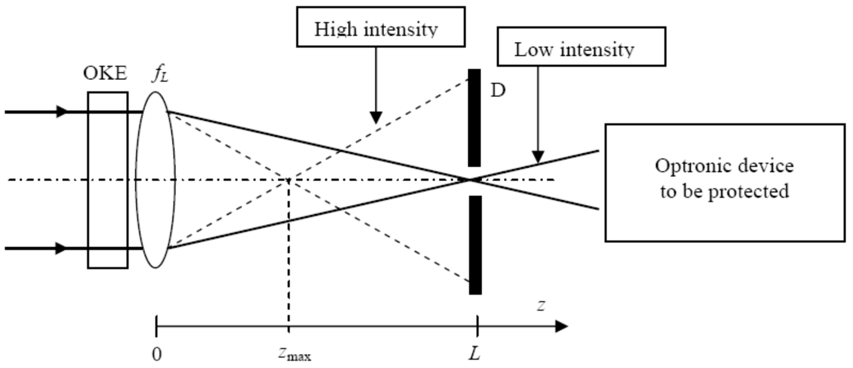
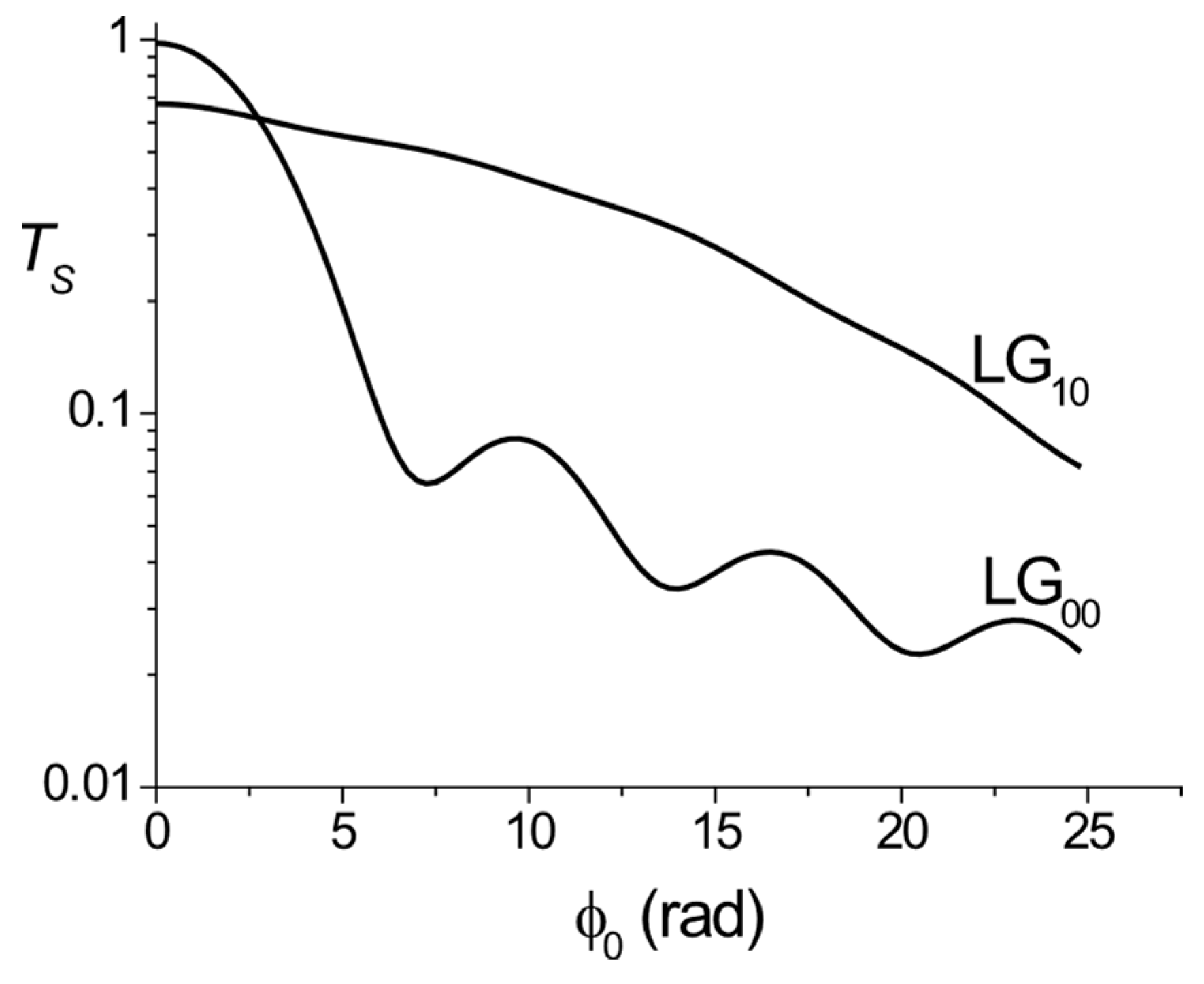
3.2. An LG10 Beam for Weakening of the Optical Limiters Protection

Before becoming involved in the issue itself, let us recall the basic principle of an optical limiter based on OKE. The aim of this system is to protect imaging devices such as optronic systems or human eyes from excessive light levels originating from an accidental or hostile laser illumination. There are several concepts of optical limiters described in [56]. Our goal is to focus on a particular family of optical limiters based on the mechanism of the Kerr lens effect, whose schematic layout is shown in Figure 20. For high (low) input intensities, the trajectory of the light follows the dashed (solid) line giving rise to a low (high) transmission through the diaphragm. The optical limiter comprises a Kerr medium of thickness d having a nonlinear refractive index n 2 , a linear lens of focal length fL = 125 mm, and a circular aperture D of radius R D . The diaphragm is set at a distance L from the focusing lens. It is important to note that the value of distance L is relatively critical since, as shown recently [57], the device shown in Figure 20 behaves like a saturable absorber if L < f L and as a limiting device if L f L . The difference between the two situations is that the aperture transmission increases (decreases) with increasing input power for a saturable absorber (optical limiter) behaviour.
Much of the work conducted in the concept of limiting systems based on OKE was carried out in the late 1980s and early 1990s [20,21,22,23,24,58,59]; however, it was assumed that the illuminating laser beam was Gaussian in shape. A careful examination of plots in Figure 13 and Figure 14 allows us to see that an optical limiter such as that drawn in Figure 20 could actually be less effective in the case where the incident Gaussian beam is replaced by a high order L G p 0 beam. It is, in a way, a countermeasure against optical limiters based on OKE. In order to set down this idea, we compare the performance of the set-up shown in Figure 20 when enlightened by a L G 00 or a L G 10 beam. The performance of the set-up shown in Figure 20 can be characterised by the transmittivity of the diaphragm D. The latter noted T S ( T D ) corresponds to a static study (dynamic study) when the incident laser beam is a continuous wave (pulse).
Static study:
The static transmittivity of the diaphragm is defined as the ratio of transmitted and incident powers:
T S = 0 R D r I d ( r , f L ) d r 0 r I d ( r , f L ) d r
The result shown in Figure 21 displays the variations of T S versus ϕ 0 , the nonlinear on-axis phase shift, which is proportional to the incident power P i n , according to Equation (6). The plots in Figure 21 are based on a logarithmic scale and demonstrate that the transmitted power P o u t = T S × P i n after the diaphragm can be higher for an L G 10 beam than for an L G 00 beam, so that the optical limitation based on OKE becomes less efficient. The value of the diaphragm radius R D is selected so that its initial static transmittivity [ T S ] i n i , for an L G 00 beam and without OKE, is equal to 98%. The relationship between [ T S ] i n i and R D is given as follows:
[ T S ] i n i = 1 exp 2 π W R D λ f L 2
It is useful to recall the four basic requirements for sensor-protecting optical limiters:
-
The protecting device has to be almost transparent in the visible and the near-infrared.
-
The response time of the limiter has to be in the picosecond (or less) range.
-
The spectral response of the limiter has to be large.
-
The nonlinear material used in the limiter must be resistant to permanent optical damage.
After the results shown in Figure 21, it is reasonable to add a supplementary condition that would impose an effective protection whatever the spatial shape of the illuminating laser beam. Nevertheless, this remains a challenging issue but absolutely important for protecting expensive optronic equipment on tomorrow’s battlefield.
Dynamic study:
From the study presented in Section 3.1, it is easy to guess that the instantaneous ratio of out- and input powers on the diaphragm is time dependent. In this case, it is preferable to define the diaphragm transmittivity T D in the dynamic case through a ratio of output and input energies:
T D = 0 R D r × F ( r ) × d r 0 r × F ( r ) × d r
The energy fluence F ( r ) is given by Equation (34). The results are shown in Figure 22, which displays the variations of T D versus the nonlinear on-axis phase shift where the conclusion is identical to that obtained when considering Figure 21: The protection of the optical limiter shown in Figure 20 is more effective for an L G 10 than for an L G 00 beam whether the aggressive laser beam is continuous or pulsed.

4. Conclusions

The research on high-order transverse modes in lasers was largely abandoned a few years after the invention of the laser in 1960. The main reason of this was that high-order beams are more divergent and less bright than the Gaussian beam for a given power. This is disqualifying in a certain number of laser applications that would be tedious to describe here. However, recently, we showed that the use of high-order radial Laguerre–Gauss beams, L G p 0 beams, can offer some advantages over the usual Gaussian L G 00 beam [50]. In the present paper, we showed that the behaviour of L G p 0 beams faced to the optical Kerr effect (OKE) varies considerably depending on the mode order (p = 0 or p 1 ). We focused our attention on the properties of L G 00 and L G 10 beams when subject to OKE, and we found that the L G 10 beam keeps its focusability much better than the L G 00 beam.
The first application is the possibility to maintain in high intensity laser chains a high focusability of the amplified pulses, despite the presence of the optical Kerr effect, even with a large breakup integral B (or ϕ 0 ). This result could be obtained by replacing the usual Gaussian beam by an L G 10 beam.
The second application concerns military defence or civil security involving the protection of the human eyes or optical systems against high intensity laser beams able to cause harmful damage. This protection is generally achieved by optical limiters based for instance on OKE, which works relatively well when the illuminating beam is Gaussian in shape. However, we showed that this protection collapses if the illuminating beam is an L G 10 beam, and this property could be considered as a counter measure against the presence of an optical limiter based on OKE.
The consequence of the early rejection of high-order modes is that most of commercial lasers still deliver a Gaussian beam, and, consequently, obtaining a high-order transverse mode L G p 0 necessitates the building of a homemade laser, including an amplitude or phase mask for forcing the laser oscillation to be a pure L G p 0 beam. Recently, a detailed study on the modelling of a cavity including a binary amplitude or a phase mask was published [60].

Author Contributions

Conceptualization, K.A.-A.; methodology, K.A.-A.; software, K.A.-A. and A.H.; validation, K.A.-A. and A.H.; format analysis, A.H. and K.A.-A.; investigation, A.H. and K.A.-A.; resources, A.H. and K.A.-A.; data curation, A.H. and K.A.-A.; writing-original draft preparation, K.A.-A.; writing-review and editing, A.H. and K.A.-A.; visualisation, A.H. and K.A.-A.; supervision, K.A.-A. All authors have read and agreed to the published version of the manuscript.

Funding

This research received no external funding.

Institutional Review Board Statement

Not applicable.

Informed Consent Statement

Not applicable.

Data Availability Statement

Data are contained within the article.

Acknowledgments

This work is dedicated to the memory of two Algerian researchers D. Louhibi (Laser technology), and T. Kerdja (Plasma physics).

Conflicts of Interest

The author declares no conflicts of interest.

Appendix A

The aberration coefficients of a phase aberration profile (PAP).
The collimated incident Gaussian beam passing through the PAP (see Figure 1) will have its wavefront degraded and then will be aberrated (non a plane and nor a sphere). It is assumed that the phase profile as the incident collimated Gaussian beam has cylindrical symmetry. The propagation term of the wave emerging from the PAP is noted exp [ i k S ( ρ ) ] , where k S ( ρ ) = ϕ ( ρ ) in order to satisfy Equation (2). The phase term S ( ρ ) is usually called a wave aberration function (WAF) according to the terminology of optical aberration modelling popularised by V.N. Mahajan [61]. The WAF is expanded as a linear combination of Zernike polynomials (ZP), noted Z j , as follows:
S ( ρ ¯ ) = j = 1 a j Z j ( ρ ¯ )
where a j is the aberration coefficient, j is a polynomial-ordering number, and ρ ¯ = ρ / ρ 0 is the normalised radial coordinate; ρ 0 = 2 W being the radius of the unit circle introduced in Section 2. Table A1 provides the ZPs.
Table A1. Zernike polynomials allowing calculation of the aberration coefficients a1, a4, a11, a22, and a37.
j Z j Type of Aberration
4 3 ( 2 ρ ¯ 2 1 ) Defocus
11 5 ( 6 ρ ¯ 4 6 ρ ¯ 2 + 1 ) Primary spherical
22 7 ( 20 ρ ¯ 6 30 ρ ¯ 4 + 12 ρ ¯ 2 1 ) Secondary spherical
37 3 ( 70 ρ ¯ 8 140 ρ ¯ 6 + 90 ρ ¯ 4 20 ρ ¯ 2 + 1 ) Tertiary spherical
The Zernike polynomials Z j ( ρ ¯ ) are a set of orthogonal functions over the unit circle ( 0 ρ 1 ) ), and consequently we can compute the ajs as the projection (inner product) of the WAF on each basis function as follows
For a plane wave [62]:
a j = λ π 0 1 ϕ ( ρ ¯ ) Z j ( ρ ¯ ) ρ ¯ d ρ ¯
For a Gaussian beam [63]:
a j = 0 1 E i n ( ρ ¯ ) ϕ ( ρ ¯ ) Z j ( ρ ¯ ) ρ ¯ d ρ ¯ k 0 1 E i n ( ρ ¯ ) ρ ¯ d ρ ¯
For convenience we can use the dimensionless aberration coefficients Aj which are expressed in unit of wavelength and given by the following:
A j = a j / λ
Note that the aberration coefficients given by Equations (A2) and (A3) can be very different as shown in Table A2.
Table A2. Dimensionless aberration coefficient associated to a phase aberration ϕ ( ρ ) = ϕ 0 exp ( 2 ρ 2 / W 2 ) when the incident wave is plane or Gaussian of width W = 1 mm and λ = 1064 nm.
Incident wave A 4 / ϕ 0 A 11 / ϕ 0 A 22 / ϕ 0 A 37 / ϕ 0
Plane wave + 7.27 × 10 2 3.38 × 10 2 + 1.08 × 10 2 2.61 × 10 3
Gaussian beam + 7.80 × 10 2 7.04 × 10 2 + 4.96 × 10 2 2.88 × 10 2
By examining Table A1, it can be seen that only the “defocus term” (j = 4) has to be considered as a pure lensing effect due to its quadratic dependence. However, it can also be seen that the high-order spherical aberrations contain a quadratic term. This is why we can define several equivalent focal lengths ( f 1 f 2 f 3 f 4 ) as demonstrated in [33]. We have first to determine the aberration coefficients of a WAF noted SL representing the wavefront of a plane wave emerging from a lens of focal length f:
S L = ρ 2 2 f = ρ ¯ 2 ρ 0 2 2 f
It is easy to show that by applying Equation (A2) the aberration coefficients characterising the WAF SL are as follows:
a 11 = a 22 = a 37 = 0 and   a 4 = ρ 0 2 3 12 f = ρ 0 2 4 3 f
As a consequence to a normalised defocus coefficient A 4 = a 4 / λ and it corresponds to a lensing effect of focal length noted f 1 given by the following:
f 1 = ρ 0 2 4 λ 3 A 4
As said before, the spherical aberrations affect the focusing of the beam at least due to the presence of quadratic terms in Z 11 , Z 22 , and Z 37 . Consequently, we can obtain several mean focal lengths [33] by taking into account the presence of the quadratic terms in the primary, secondary, and tertiary aberration coefficients. Finally, we obtain the following:
f 2 = ρ 0 2 2 λ 2 3 A 4 6 5 A 11
f 3 = ρ 0 2 2 λ 2 3 A 4 6 5 A 11 + 12 7 A 22
f 4 = ρ 0 2 2 λ 2 3 A 4 6 5 A 11 + 12 7 A 22 60 A 37

References

  1. Campillo, A.; Shapiro, S.; Suydam, B. Periodic breakup of optical beams due to self-focusing. Appl. Phys. Lett. 1973, 23, 628–630. [Google Scholar] [CrossRef]
  2. Feit, M.; Fleck, J. Beam nonparaxiality, filament formation, and beam breakup in the self-focusing of optical beams. JOSA B 1988, 5, 633–640. [Google Scholar] [CrossRef]
  3. Magni, V.; Cerullo, S.; DeSilvestri, S. ABCD matrix analysis of propagation of Gaussian beams through Kerr media. Opt. Commun. 1993, 96, 348–355. [Google Scholar] [CrossRef]
  4. Hermann, J. Theory of Kerr-Lens mode locking: Role of self-focusing and radially varying gain. JOSA B 1994, 11, 498–512. [Google Scholar] [CrossRef]
  5. Yefet, S.; Pe’er, A. A review of cavity design for Kerr Lens mode-locked solid-state lasers. Appl. Sci. 2013, 3, 694–724. [Google Scholar] [CrossRef]
  6. Akbari, R.; Major, A. Kerr-lens mode locking of a diode-pumped Yb:KGW laser using an additional intracavity Kerr medium. Las. Phys. Lett. 2018, 15, 085001. [Google Scholar] [CrossRef]
  7. Levine, Z.H.; Du, Z. Semiclassical calculation of the power saturation of the Kerr effect in Rb vapor. JOSA B 2023, 40, 3190–3195. [Google Scholar] [CrossRef]
  8. Robertson, S. Optical Kerr effect in vacuum. Phys. Rev. A 2019, 100, 063831. [Google Scholar] [CrossRef]
  9. Hsieh, T.; Lee, D.S.; Lin, C.Y. Throat effects on strong gravitational lensing in Kerr-like wormholes. Phys. Rev. D 2025, 111, 044051. [Google Scholar] [CrossRef]
  10. Gralla, S.E.; Lupsasca, A. Lensing by Kerr black holes. Phys. Rev. D 2020, 101, 044031. [Google Scholar] [CrossRef]
  11. Siegman, A. Analysis of laser beam quality degradation caused by quartic phase aberrations. Appl. Opt. 1993, 32, 5893–5901. [Google Scholar] [CrossRef] [PubMed]
  12. Ruff, J.A.; Siegman, A.E. Measurement of beam quality degradation due to spherical aberration in a simple lens. Opt. Quantum Electron. 1994, 26, 629–632. [Google Scholar] [CrossRef]
  13. Pu, J.; Zhang, H. Intensity distribution of Gaussian beams focused by a lens with spherical aberration. Opt. Commun. 1998, 151, 331–338. [Google Scholar] [CrossRef]
  14. Karman, G.P.; Van Duijl, A.; Woerdman, J.P. Observation of a stronger focus due to spherical aberration. J. Mod. Opt. 1998, 45, 2513–2517. [Google Scholar] [CrossRef]
  15. Ji, X.; Lü, B. Focal shift of flattened Gaussian beams passing through a spherically aberrated lens. Optik 2002, 113, 201–204. [Google Scholar] [CrossRef]
  16. Escobar, I.; Saavedra, G.; Martinez-Corral, M. Reduction of the spherical aberration effect in high-numerical-aperture optical scanning instruments. JOSA A 2006, 23, 3150–3155. [Google Scholar] [CrossRef]
  17. Alkelly, A. Spot size and radial intensity distribution of focused Gaussian beams in spherical and non-spherical aberration lenses. Opt. Commun. 2007, 277, 397–405. [Google Scholar] [CrossRef]
  18. Singh, R.; Senthilkumaran, P.; Singh, K. Focusing of a singular beam in the presence of spherical aberration and defocusing. Optik 2008, 119, 459–464. [Google Scholar] [CrossRef]
  19. George, J.; Seihgal, R.; Oak, S.M.; Mehendale, S.C. Beam quality degradation of a higher order transverse mode beam due to spherical aberration of a lens. Appl. Opt. 2009, 48, 6202–6206. [Google Scholar] [CrossRef]
  20. Soileau, M.; Williams, W.; Van Stryland, E. Optical power limiter with picosecond response time. IEEE J. Quant. Electron. 1983, 19, 731–735. [Google Scholar] [CrossRef]
  21. Hermann, J. Beam propagation and optical power limiting with nonlinear media. JOSA B 1984, 1, 729–736. [Google Scholar] [CrossRef]
  22. Hermann, J. Simple model for a passive optical power limiter. Opt. Acta 1985, 32, 541–547. [Google Scholar] [CrossRef]
  23. Hermann, J. External self-focusing, self-bending and optical limiting with thin non-linear media. Opt. Quant. Electron. 1987, 19, 169–178. [Google Scholar] [CrossRef]
  24. Sheik-Bahae, M.; Said, A.; Hagan, D.; Soileau, M.; Van Stryland, E. Simple analysis and geometric optimization of a passive optical limiter based on internal sel-action. Proc. SPIE 1989, 1105, 146–153. [Google Scholar]
  25. Bliss, E.S.; Hunt, J.T.; Renard, P.A.; Sommargren, G.E.; Weaver, H.J. Effects of nonlinear propagation on laser focusing properties. IEEE J. Quantum Electron. 1976, 12, 402–406. [Google Scholar] [CrossRef]
  26. Glaze, J.A. High energy glass lasers. Opt. Eng. 1976, 15, 152136. [Google Scholar] [CrossRef]
  27. Yu, B.; Chen, X.; Qiu, W.; Pu, J. Impact of nonlinear Kerr effect on the focusing performance of optical lens with high-intensity laser incidence. Appl. Sci. 2020, 10, 1945. [Google Scholar] [CrossRef]
  28. Kogelnik, H. Imaging of optical modes-resonators with internal lenses. Bell Syst. Tech. J. 1965, 44, 455–494. [Google Scholar] [CrossRef]
  29. Guo, P.; Schaller, R.D.; Ocola, L.E.; Diroll, B.T.; Ketterson, J.B.; Chang, R. Large optical nonlinearity of ITO nanorods for subpicosecond all-optical modulation of the full-visible spectrum. Nat. Commun. 2016, 7, 12892. [Google Scholar] [CrossRef]
  30. Pinçon-Roetzinger, N.; Prot, D.; Palpant, B.; Charron, E.; Debrus, S. Large optical Kerr effect in matrix-embedded metal nanoparticles. Mat. Sci. Eng. C 2002, 19, 51–54. [Google Scholar] [CrossRef]
  31. Genchi, D.; Dodici, F.; Cesca, T.; Mattei, G. Design of optical Kerr effect in multilayer hyperbolic metamaterials. Nanophotonics 2024, 13, 4523–4536. [Google Scholar] [CrossRef]
  32. Alam, M.Z.; Schulz, S.A.; Upham, J.; De Leon, I.; Boyd, R.W. Large optical nonlinearity of nanoantennas coupled to an epsilon-near-zero material. Nat. Photonics 2018, 12, 79–83. [Google Scholar] [CrossRef]
  33. Mafusire, C.; Forbes, A. Mean focal length of an aberrated lens. JOSA A 2011, 28, 1403–1409. [Google Scholar] [CrossRef]
  34. Leghmizi, S.; Hasnaoui, A.; Boubaha, B.; Aissani, A.; Ait-Ameur, K. On the effective ways for defining the effective focal length of a Kerr lens effect. Laser. Phys. 2017, 27, 106201. [Google Scholar] [CrossRef]
  35. Hall, D.R.; Jackson, P.E. The Physics and Technology of Laser Resonators; Institute of Physics Publishing: Bristol, UK, 1989; Chapter 9. [Google Scholar]
  36. Haddadi, S.; Bouzid, O.; Fromager, M.; Hasnaoui, A.; Harfouche, A.; Cagniot, E.; Forbes, A.; Aït-Ameur, K. Structured Laguerre-Gaussian beams for mitigation of spherical aberration in tightly focused regimes. J. Opt. 2018, 20, 045602. [Google Scholar] [CrossRef]
  37. Ait-Ameur, K.; Hasnaoui, A. Improving the longitudinal and radial forces of optical tweezers: A numerical study. Opt. Commun. 2024, 551, 130033. [Google Scholar] [CrossRef]
  38. Yoshida, A.; Asakura, T. Propagation and focusing of Gaussian laser beams beyond conventional diffraction limit. Opt. Commun. 1996, 123, 694–704. [Google Scholar] [CrossRef]
  39. Caumes, J.; Videau, L.; Rouyer, C.; Freysz, E. Direct measurement of wave-front distortion induced during secon-harmonic generation: Application to breakup-integral compensation. Opt. Lett. 2004, 29, 899–901. [Google Scholar] [CrossRef]
  40. Khoo, I.C.; Hou, J.Y.; Yan, T.H.; Michael, R.R.; Finn, G.M. Transverse self-phase modulation and bistability in the transmission of a laser beam through a nonlinear thin film. JOSA B 1987, 4, 886–891. [Google Scholar] [CrossRef]
  41. Marburger, J.H. Self-focusing: Theory. Prog. Quantum Electron. 1975, 4, 35–110. [Google Scholar] [CrossRef]
  42. Simmons, W.W.; Hunt, J.T.; Warren, W.E. Light propagation through large laser systems. IEEE J. Quantum Electron. 1981, 17, 1727–1744. [Google Scholar] [CrossRef]
  43. Simmons, W.; Speck, D.; Hunt, J. Argus laser system: Performance summary. Appl. Opt. 1978, 17, 999–1005. [Google Scholar] [CrossRef]
  44. Simmons, W.; Godwin, R. Nova laser fusion facility design, engineering, and assembly overview. Nucl. Technol. Fusion 1983, 4, 8–24. [Google Scholar] [CrossRef]
  45. Kuz’mina, N.B.; Rozanov, N.N.; Smirnov, V.A. On spatial filtration of apodized laser beams. Opt. Spectro. 1981, 51, 509–514. [Google Scholar]
  46. Deng, J.; Ji, X. Influence of atmospheric turbulence on the energy focusability of Gaussian beams with spherical aberration. J. Opt. 2014, 16, 055705. [Google Scholar] [CrossRef]
  47. Weberpais, J.; Dausinger, F.; Göbel, G.; Brener, B. The role of strong focusability on the welding process. In Proceedings of the ICALEO 2006: 25th International Congress on Laser Materials Processing and Laser Microfabrication, Scottsdale, AR, USA, 30 October–2 November 2006; paper#905. pp. 553–560. [Google Scholar] [CrossRef]
  48. Mahajan, V.N. Strehl ratio of a Gaussian beam. JOSA A 2005, 22, 1824–1833. [Google Scholar] [CrossRef]
  49. Jabczynski, J.K.; Kaskow, M.; Gorajek, L.; Kopczynski, K.; Zendzian, W. Modeling of the laser beam shape for high-poer applications. Opt. Eng. 2018, 57, 046107. [Google Scholar] [CrossRef]
  50. Aït-Ameur, K. The advantages and disadvantages of using structured high-order but single Laguerre-Gauss LGp0 laser beams. Photonics 2024, 11, 217. [Google Scholar] [CrossRef]
  51. Boyd, R.W.; Lukishova, S.G.; Shen, Y.R. Self-Focusing: Past and Present, Fundamentals and Prospects; Topics in Applied Physics; Springer: Berlin/Heidelberg, Germany, 2009; Volume 114, Chapter 8. [Google Scholar]
  52. Campillo, A.J.; Fisher, R.A.; Hyer, R.C.; Shapiro, L. Streak camera investigation of the self-focusing onset in glass. Appl. Phys. Lett. 1974, 25, 408–410. [Google Scholar] [CrossRef]
  53. Maine, P.; Strickland, D.; Bado, P.; Pessot, M.; Mourou, G. Generation of ultrahigh peak power pulses by chirped pulse amplification. IEEE J. Quantum Electron. 1988, 24, 398–403. [Google Scholar] [CrossRef]
  54. Mourou, G. The ultrahigh-peak-power laser: Present and future. Appl. Phys. B 1997, 65, 205–211. [Google Scholar] [CrossRef]
  55. Mourou, G.; Fish, N.J.; Malkin, V.N.; Toroker, Z.; Khazanov, E.A.; Sergeev, A.M.; Tajima, T.; Le Garrec, B. Exawatt-Zettawatt pulse gerenation and applications. Opt. Commun. 2012, 285, 720–724. [Google Scholar] [CrossRef]
  56. Tutt, L.W.; Boggess, T.F. A review of optical limiting mechanisms and devices using organic, fullerenes, semiconductors and other materials. Prog. Quant. Electron. 1993, 17, 299–338. [Google Scholar] [CrossRef]
  57. Hasnaoui, A.; Ait-Ameur, K. Simple modelling of nonlinear losses induced by Kerr lensing effect. Appl. Phys. B 2021, 127, 100. [Google Scholar] [CrossRef]
  58. Hermann, J. Self-focusing effects and applications using thin nonlinear media. Int. J. Nonlinear Opt. Phys. Mat. 1992, 1, 541–561. [Google Scholar] [CrossRef]
  59. Hermann, J.; Wilson, P. Factors affecting optical limiting and scanning with thin nonlinear samples. Int. J. Nonlinear Opt. Phys. Mat. 1993, 2, 613–629. [Google Scholar] [CrossRef]
  60. Aït-Ameur, K.; Fromager, M.; Hasnaoui, A. Numerical simulation of an optical resonator for the generation of radial Laguerre-Gauss LGp0 modes. Appl. Sci. 2025, 15, 3331. [Google Scholar] [CrossRef]
  61. Mahajan, V.N. Optical Imaging and Aberrations; SPIE Optical Engineering Press: Bellingham, WA, USA, 1998. [Google Scholar]
  62. Mahajan, V.N. Zernike circle polynomials and optical aberrations of system with circular pupils. Appl. Opt. 1994, 33, 8121–8124. [Google Scholar] [CrossRef]
  63. Mahajan, V.N. Zernike-Gauss polynomials and optical aberrations of systems with Gaussian pupils. Appl. Opt. 1995, 34, 8057–8059. [Google Scholar] [CrossRef]
Figure 1. Set-up showing the geometry of the diffraction of a collimated Gaussian beam subject to optical Kerr effect (OKE).
Photonics 12 00596 g001
Figure 2. Relative variation in z max , the position of the best focus, versus the on-axis nonlinear phase shift ϕ 0 . The plot in the black colour corresponds to the calculation of z max using the diffraction integral. The plot in the red colour results from the parabolic approximation.
Photonics 12 00596 g002
Figure 3. Variations of Kerr focal length f K versus W 2 for ϕ 0 = π .
Photonics 12 00596 g003
Figure 4. Variations of the Kerr focal length f K determined by using Equation (10) versus ϕ 0 1 (in black) for W = 1 mm. The linear fit is in red colour.
Photonics 12 00596 g004
Figure 5. Variations of the Kerr focal lengths f K and f j (j = 1–4) versus ϕ 0 1 .
Photonics 12 00596 g005
Figure 6. Variations of the on-axis intensity in the focal plane z = f L versus ϕ 0 for a Gaussian beam subject to optical Kerr effect.
Photonics 12 00596 g006
Figure 7. Schematic of the set-up allowing for modelling the variations of the on-axis intensity in plane P resulting from the expansion of the Gaussian beam focalised in plane P′.
Photonics 12 00596 g007
Figure 8. Variations of the Kerr focal length versus the nonlinear on-axis phase shift.
Photonics 12 00596 g008
Figure 9. On-axis intensity distribution I d ( r , z ) = E d ( r , z ) 2 of a collimated Gaussian beam of width W = 1 mm diffracted by a phase profile Δ ϕ ( ρ ) = ϕ 0 exp [ 2 ρ 2 / W 2 ] and focused by a linear lens of focal length fL = 50 mm.
Photonics 12 00596 g009
Figure 10. Radial intensity distribution in the plane z = f L for several values of the nonlinear phase shift.
Photonics 12 00596 g010
Figure 11. Variation of the M 2 factor of the Gaussian beam traversing the Gaussian Kerr lens versus the nonlinear on-axis phase shift ϕ 0 . The M 2 factor is independent of the width W of the incident beam.
Photonics 12 00596 g011
Figure 12. Transverse intensity distribution of the 4-first radial Laguerre–Gauss LGp0 beams.
Photonics 12 00596 g012
Figure 13. Variations of the on-axis intensity in the plane z = f L versus ϕ 0 the nonlinear on-axis phase shift for the first four-Laguerre–Gauss L G p 0 beams focused by a lens of focal lens fL = 50 mm and subject to OKE.
Photonics 12 00596 g013
Figure 14. Variations in the relative variations in z max , the longitudinal position of the best focus, versus the on-axis nonlinear phase shift, for the first three-high-order-Laguerre–Gauss L G p 0 beams focused by a lens of focal lens fL = 50 mm and subject to OKE.
Photonics 12 00596 g014
Figure 15. Variations of the Strehl ratio S of a L G p 0 beam subject to optical Kerr effect characterised by an on-axis nonlinear phase shift ϕ 0 .
Photonics 12 00596 g015
Figure 16. Longitudinal distribution of the on-axis intensity of focused L G 00 and L G 10 beams by a lens of focal length f L = 125 mm, and subject to optical Kerr effect for the following: (a) ϕ 0 = 0 , (b) ϕ 0 = 2 π , (c) ϕ 0 = 4 π . Although the on-axis axes are expressed in arbitrary units, they are comparable.
Photonics 12 00596 g016
Figure 17. Transverse intensity distribution I d ( r , z = f L ) for ϕ 0 = 6 rad and 12 rad: (a) p = 0 and ϕ 0 = 6 rad, (b) p = 1 and ϕ 0 = 6 rad, (c) p = 0 and ϕ 0 = 12 rad, (d) p = 1 and ϕ 0 = 12 rad.
Photonics 12 00596 g017
Figure 18. Variations of the focused on-axis intensity in plane z = f L versus the normalised time t / τ of L G 00 and L G 10 beams subject to OKE: (a) ϕ 0 = 0 , (b) ϕ 0 = 6 rad, (c) ϕ 0 = 12 rad.
Photonics 12 00596 g018
Figure 19. Variations of the energy fluence distribution in plane z = f L for three values of ϕ 0 : (a) p = 0, and (b) p = 1. ϕ 0 is the nonlinear phase shift at the temporal peak of the incident beam. The calculations are made for a focal length fL = 125 mm.
Photonics 12 00596 g019
Figure 20. Schematic layout of an optical limiter based on OKE. It is made up of a Kerr medium, a linear lens of focal length f L , a diaphragm D of radius R D : solid line—low input power, dashed line—high input power. The best focus is located at z = f L ( z = z max ) for a low (high) power.
Photonics 12 00596 g020
Figure 21. Variations of the static transmittivity T S of the optical limiter versus the nonlinear phase shift. The parameters of the calculations are the following: fL = 125 mm, W = 1 mm, λ = 1064 nm, [ T S ] i n i = 98 % .
Photonics 12 00596 g021
Figure 22. Variations of the dynamic transmittivity T D versus the nonlinear on-axis phase shift. The parameters used are identical to that used in Figure 21.
Photonics 12 00596 g022
Disclaimer/Publisher’s Note: The statements, opinions and data contained in all publications are solely those of the individual author(s) and contributor(s) and not of MDPI and/or the editor(s). MDPI and/or the editor(s) disclaim responsibility for any injury to people or property resulting from any ideas, methods, instructions or products referred to in the content.

