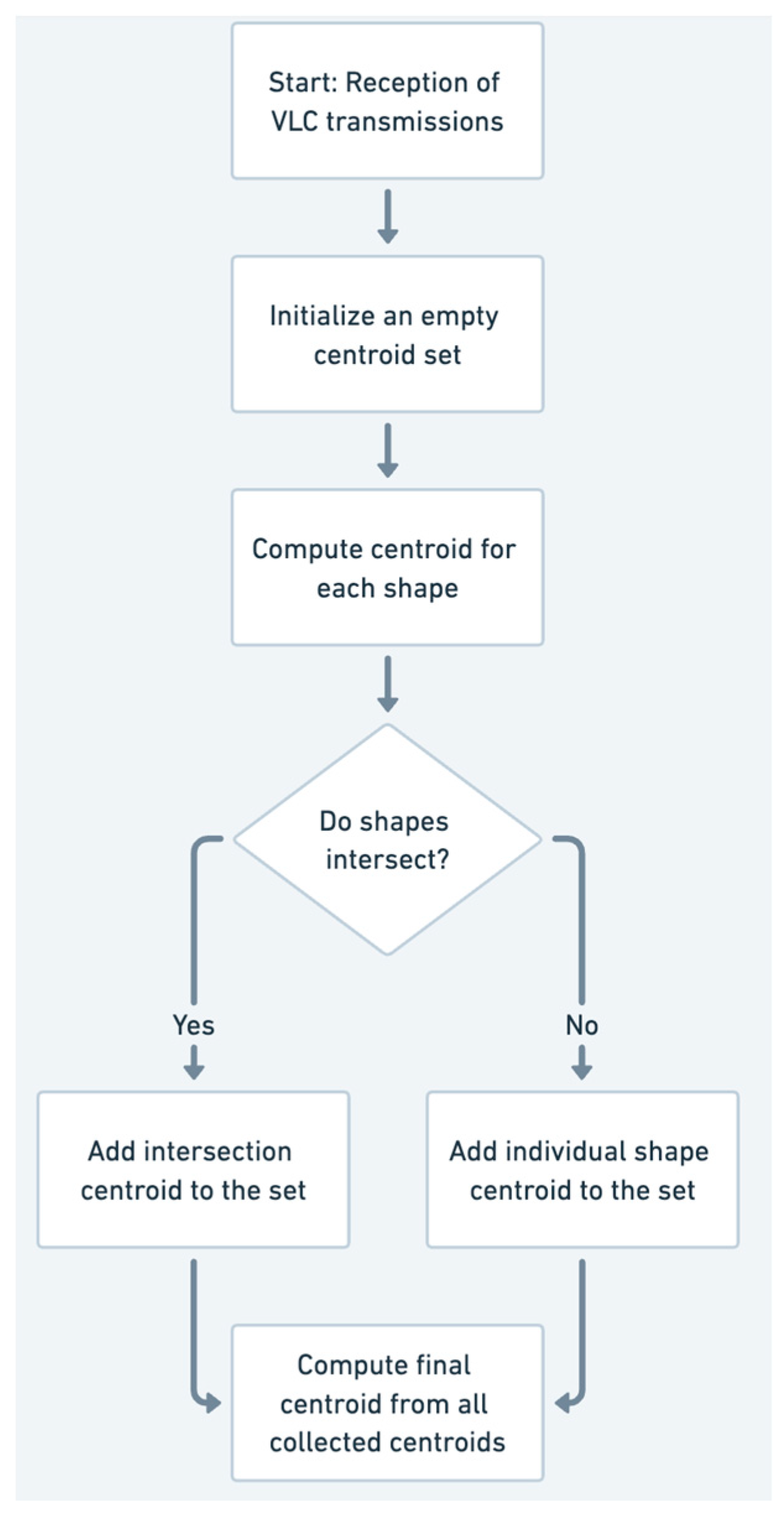
Article

Three-Dimensional Localization of Underwater Nodes Using Airborne Visible Light Beams

Department of Computer Science and Electrical Engineering, University of Maryland Baltimore County, Baltimore, MD 21250, USA
*
Author to whom correspondence should be addressed.
Photonics 2025, 12(5), 503; https://doi.org/10.3390/photonics12050503
Submission received: 26 March 2025 / Revised: 1 May 2025 / Accepted: 16 May 2025 / Published: 18 May 2025

Abstract

:
Localizing underwater nodes when they cannot be tethered or float on the surface presents significant challenges, primarily due to node mobility and the absence of fixed anchors with known coordinates. This paper advocates a strategy for tackling such a challenge by using visible light communication (VLC) from an airborne unit. A novel localization method is proposed where VLC transmissions are made towards the water surface; each transmission is encoded with the Global Positioning System (GPS) coordinates with the incident point of the corresponding light beam. Existing techniques deal with the problem in 2D by assuming that the underwater node has a pressure sensor to measure its depth. The proposed method avoids this limitation and utilizes the intensity of VLC signals to estimate the 3D position of the underwater node. The idea is to map the light intensity at the underwater receiver for airborne light beams and devise an error optimization formulation to estimate the 3D coordinates of the underwater node. Extensive simulations validate the effectiveness of the proposed method and capture its performance across various parameters.

1. Introduction

The relentless advancement of communication technologies has dramatically transformed our capacity to interact with and understand the world around us. A significant contributor to this transformation is the Internet of Things (IoT), which envisions a seamlessly connected network of devices operating across diverse environments, including terrestrial, aerial, and aquatic domains. As we move towards the next generation of wireless technology with the emergence of 6G, the integration of underwater networks has become increasingly important. These networks hold the key to a multitude of critical applications such as monitoring marine life, assessing environmental pollutants, conducting oceanographic research, and executing high-priority operations like search-and-rescue missions or clandestine military surveillance.
A fundamental challenge in deploying underwater networks is the precise localization of submerged nodes. Accurate positioning is essential not only for contextualizing the collected data but also for optimizing the network topology and boosting the efficiency of communication protocols. Traditional localization methods have predominantly utilized acoustic signaling [1,2], relying on surface vessels or anchored nodes with GPS coordinates to translate relative positions into global coordinates. However, in scenarios where operational stealth is required—such as in covert naval operations—the presence of surface or tethered markers can compromise the mission by revealing the presence of the underwater network [3,4]. In addition, deploying markers could constitute a logistical challenge in applications that serve emerging events such as search and rescue and naval combat.
To overcome these limitations, this paper proposes the use of VLC across the air–water interface as an innovative solution for underwater node localization. VLC stands out as an effective means due to its ability to transmit high-bandwidth data through both air and water, and hence it does not need the deployment of relaying nodes on the water surface. Unlike photoacoustic techniques [4], which often suffer from logistical complexities and limited data rates, VLC offers a more efficient and scalable approach. VLC eliminates the need for surface-deployed infrastructure such as buoys, anchored relays, or pressure-based markers. This not only reduces logistical burden but also removes visual and physical traces of the network from the water surface. The result is a system that is inherently well-suited for covert, rapidly deployable, and infrastructure-free localization, further enhanced by the high directionality and rapid attenuation of light in water [5], which localizes the transmission footprint and minimizes the risk of detection by unintended observers. By measuring received light intensities and applying trilateration algorithms, we demonstrate that underwater nodes can be accurately localized without the need for surface-based reference points. This method not only enhances the feasibility of deploying underwater networks in sensitive operations but also enables the introduction of new applications, e.g., studying the effect of climate change. In our preliminary investigation [6,7,8], we have assumed that the underwater node is equipped with a pressure sensor to measure its depth, effectively reducing the scope of the localization problem to 2D. However, in practice, the node may not have a pressure sensor due to constraints like power consumption, node size, or cost. This paper overcomes such a limitation and proposes 3D-LUNA, a novel method for 3D localization of underwater nodes using airborne visible light beams. This novel framework enables underwater node localization using airborne VLC without relying on pressure sensors or anchored nodes. The method reconstructs 3D positions by correlating light intensity measurements with modeled beam propagation across depth layers. To address the challenge of unknown depth, we introduce an optimization approach that identifies the most likely depth by minimizing errors. The system is validated through extensive simulations, demonstrating high localization accuracy and robustness under different deployment and mobility conditions.
It is worth noting that while recent research such as the HOENN-based DoA estimation method [9] also utilizes magnitude measurements for angular inference, its objective, methodology, and application context are fundamentally different from ours. Specifically, HOENN is designed for aerial scenarios and employs hybrid optical–electronic neural networks and diffractive metasurfaces to estimate the direction of arrival of RF signals. In contrast, our proposed 3D-LUNA framework addresses the challenge of cross-medium 3D localization of underwater nodes by modeling the propagation of visible light beams across the air–water interface. It reconstructs node coordinates based on measured light intensity without relying on learning-based architectures or angular classification. Unlike HOENN, 3D-LUNA requires no pre-training or metasurfaces and is particularly suited for infrastructure-free and covert underwater applications.
The rest of this paper is organized as follows. Section 2 provides a review of related work, discussing existing underwater localization techniques and their limitations. Section 3 presents the system model and the theoretical foundation of our proposed 3D-LUNA approach, including key assumptions and mathematical formulations. Section 4 details the 3D-LUNA localization protocol, explaining how airborne VLC beams are utilized for accurate underwater node positioning. Section 5 evaluates the proposed method through extensive simulations, analyzing its accuracy, efficiency, and robustness under various conditions. Finally, Section 6 concludes the paper by summarizing key contributions and outcomes.

2. Related Work

Accurate localization of underwater nodes is vital for applications such as marine research, environmental monitoring, and defense operations. Traditionally, acoustic-based methods have been the primary approach, as sound waves propagate efficiently in water [10,11,12]. In contrast, radio frequency (RF) and electromagnetic waves, commonly used for terrestrial and aerial localization, face significant challenges underwater [13,14]. The high conductivity of seawater causes severe attenuation of RF signals, drastically limiting their range. While extremely low frequency (ELF) and very low frequency (VLF) waves have been explored for deep-sea communication, their feasibility is hindered by the need for large antennas and high power consumption, making them unsuitable for compact underwater nodes [15]. Another alternative, magnetic induction (MI) communication, has shown promise for cross-medium applications like air-to-water transmission [16]. However, despite its ability to penetrate the water surface, MI communication suffers from substantial path loss, restricting its practical use.
Traditional underwater localization has predominantly relied on acoustic-based methods, which leverage sound waves due to their superior propagation characteristics in water. Various approaches, such as time of arrival (ToA) [17], time difference of arrival (TDoA) [18], and angle of arrival (AoA) [19], have been widely employed in underwater sensor networks. Acoustic localization systems are further classified into range-based methods [20,21,22], which require precise distance measurements between nodes, and range-free methods [23,24], which use connectivity or hop-count data to estimate positions. These techniques have been extensively studied, leading to solutions such as long baseline (LBL) [25], short baseline (SBL) [26], and ultra-short baseline (USBL) [27] systems. Despite their widespread adoption, acoustic-based methods have several limitations. First, they suffer from high latency and limited bandwidth, restricting data transmission rates [28]. Second, the presence of multipath effects, Doppler shifts, and environmental noise significantly affects accuracy [29]. Moreover, acoustic localization often relies on surface or anchored reference nodes, which may not be viable in dynamic or covert operations.
In recent years, VLC has emerged as a promising alternative to traditional acoustic and RF-based underwater communication [5,30]. Recent studies have improved the understanding of VLC channel characteristics and performance, with a particular focus on light propagation across different water conditions [31]. The behavior of light beams as they transition through air–water interfaces has been examined [32]. VLC leverages high-bandwidth optical signals to achieve low-latency, high-data-rate transmission in underwater environments [33,34]. Compared to acoustic methods, VLC offers significantly higher throughput and is not affected by Doppler shifts or multipath fading. Recent research has also investigated cross-medium VLC localization, where optical signals propagate from an airborne or surface source into the underwater environment.
Some approaches rely on passive optical uplinks to improve positioning accuracy [35]. This method typically involves placing retroreflectors or light-sensitive surfaces on underwater nodes, which reflect or modulate incoming optical signals from surface or airborne sources back to receivers. This allows for range estimation or angle-of-arrival measurements using returned light, often improving localization accuracy without requiring active transmission from the underwater node. While such systems reduce onboard power requirements and hardware complexity, they still require careful alignment between transmitters and receivers. Moreover, the optoacoustic effect has been exploited for cross-medium localization, where high-energy laser beams are used to generate underwater acoustic signals [36,37]. While these methods enable underwater signal transmission, they suffer from high power consumption and complex deployment requirements, making them less suitable for mobile or energy-constrained underwater networks. Xiaoyang et al. utilized polarization and deep learning techniques for underwater geolocation [38]; however, their approach required a vast amount of data collection. Fusion of aerial image and acoustic image using neural networks has also been explored [39], but it still relies on vast data collection and processing. Despite all the advancements, existing solutions often rely on surface nodes, pressure sensors, or passive uplinks, limiting their feasibility for real-world deployment. To the best of our knowledge, no prior study has demonstrated a fully airborne-enabled underwater localization system that transmits GPS-encoded positioning information directly to underwater nodes without relying on anchored reference points, depth sensors, or pre-collected data.

3. System Model and Analysis

This section outlines the fundamental assumptions and offers background information necessary for calculating underwater light intensity for an airborne VLC beam. It also examines and derives the intensity distribution without considering depth information for the underwater node.

3.1. System Model and Assumptions

The proposed methods enable the localization of one or more underwater nodes within a specified rectangular area. Underwater nodes can be stationary or mobile. Each node is assumed to be equipped with a VLC receiver; mobile nodes additionally are assumed to have an inertial navigation system. After the nodes are deployed, an airborne unit hovers over the area to aid in determining the global coordinates of the underwater nodes. This airborne unit is equipped with a VLC transmitter and a GPS-based locator.

3.2. Underwater Light Intensity for a Normal Light Beam

As highlighted, an airborne light beam can penetrate the water surface and propagate within it. Islam et al. [32] have investigated the underwater coverage area of a normal light beam of the water interface. Table 1 summarizes the notation used. Figure 1 depicts a scenario with a flat water surface and a uniform light source situated at point S, emitting light at an angle of θ. This light source is placed at a height of a d meters above the water surface. To evaluate the light coverage area on the water surface, we also consider an underwater sensor located at a depth of w d meters, i.e., at point J. Specifically, the light intensity at point J with respect to the light source is as follows:
I = 360 θ   .   τ   .   P 4 π a d c o s θ i 2   .   e k w d c o s θ r
According to Equation (1), the coverage area both on the water’s surface and underwater is circular, with intensity decreasing as the distance from the center point increases, whether at the surface or at a specific depth. Figure 2 illustrates the intensity distribution for a normal beam in the x-y plane. It can be inferred that the light intensity received by an underwater node is uniform along the circumference of a circle. This uniformity is due to the equal distance of all points on the perimeter from the center of the coverage area at a given depth.
When an underwater node receives an airborne VLC transmission for a known depth, by measuring the intensity the node can measure the proximity from its transmission center. The location lies on the circumference of a circle as it is equidistant from the center.

3.3. Intensity-Based Location Estimation in the Absence of Depth Information

If the underwater node is not equipped with a depth sensor, Equation (1) can have multiple solutions for different depths. To illustrate, let us rearrange Equation (1):
I . θ . 4 π . a d 2 360 . τ . P = ( c o s θ i ) 2 . e k w d c o s θ r
Let us consider the left side of the equation as a single constant I * . Since θ i and θ r are related by Snell’s law, we can substitute them with each other. So, the equation becomes the following:
I * = ( c o s θ i ) 2 . e k w d c o s ( sin 1 n a . sin θ i n w )
w d = ln I * ( c o s θ i ) 2 . c o s ( sin 1 n a . sin θ i n w ) k
Equation (4) can have multiple solutions as a pair of w d and θ i . The underwater depth, defined as a function of w d and θ i , will provide us with the incident angle, which can be translated into the distance from the center at that depth. From Figure 1,
D J ¯ = D H ¯ + H J ¯ = a d . tan θ i + w d . tan θ r
θ r can be calculated from θ i , since the reflectance coefficient is known for both water and air.
s i n θ r = n a n w . s i n θ i
Equation (4) may not be valid for all possible depths; depending on the other values, it may provide valid solution pairs for only certain depths specifically for the argument of the inverse sine function to be valid. We can discretize the depth value and find the solutions for the proximity of the corresponding depth for a received and measured intensity. Figure 3 illustrates the possible location of the underwater node in the case that the underwater node depth is unknown. Each circle at each depth represents the possible location of the underwater node. All the circles combined form this 3D contour, which represents all the possible locations of the underwater node. Now, depending on the parameters like transmission power and received transmission intensity, this 3D contour can be wider or thinner and taller or shorter.

4. The 3D-LUNA Localization Framework

To establish a global coordinate system for underwater networks, anchor nodes with predetermined positions must be deployed. Conventionally, these anchors can either be tethered underwater nodes or floating surface nodes. However, as noted in Section 1, deploying these anchors could be impractical in many underwater applications. This paper overcomes this serious shortcoming and proposes a more efficient approach utilizing air-to-water cross-medium communication. This section outlines how VLC can be applied to this task.

4.1. Virtual Anchor Creation

Localization relies on determining relative positions, which represent the topological relationships between network nodes. To obtain global coordinates for a node, its relative position must be linked to anchors/reference points with known coordinates. Rather than deploying tethered underwater nodes or surface nodes, our approach involves defining uniformly spaced waypoints throughout the operational area and transmitting encoded visual light beams to each of these points. The airborne node divides the water surface into a grid of square cells, hovering above to illuminate each of these cells with a light beam that encodes its current GPS coordinates. This encoded position provides the underwater nodes with the x and y coordinates where the beam hits the surface, along with the airborne node’s altitude (z coordinate). Additionally, the airborne node includes other vital data like the beam angle and transmission power, enabling the underwater nodes to use this information, in conjunction with Equation (4), to calculate the full 3D position from each transmission, as explained in the balance of this section. Since the airborne node covers the entire region with sequential cell by cell transmission, necessary coverage is achieved by a single airborne node.

4.2. Localization of Nodes with Known Depth

In our previous work [4], we demonstrated the localization process of stationary underwater nodes with known depth. The assumption was that the underwater node is equipped with a pressure sensor that can measure the underwater depth of the node. So, rather than getting a 3D contour as depicted in Figure 3, we end up with a single circle in the x-y plane which shows the position of the underwater node after receiving a VLC transmission and measuring its intensity. As the airborne node is transmitting cell by cell and the VLC transmission is spreading underwater due to its beam angle, the underwater node may end up receiving multiple transmissions and multilaterate the ranges to find out its x and y coordinates. In other words, in the case of known depth, the multilateration process is simple as the sensor position is represented by a 2D circle in the x-y plane. Upon receiving multiple transmissions, the intersection between the measured circles would represent the sensor position. To localize the sensor to a single point, three or more transmissions are needed. As the absence of depth information leads to a 3D contour as opposed to a 2D circle, the multilateration process will be more complicated, as explained below.

4.3. Handling Unknown Depth

When a node receives a single transmission, Figure 3 represents the possible location of the node where the node can be located anywhere on the surface of a 3D shape. Therefore, to determine the node’s position, multiple transmissions should be received, and the corresponding 3D contours are correlated. In essence, we need to find the intersection of at least three contours to determine the x, y, and z coordinates of the underwater node. Later in this section, we will discuss the scenarios in which fewer transmissions are received.
Figure 4 illustrates the fundamental principle behind the multilateration process used in 3D-LUNA when the underwater node’s depth is unknown. Each VLC transmission produces a 3D contour of potential positions (as shown previously in Figure 3), and these are discretized into circular slices at various depths. If a node receives three or more transmissions, in an ideal scenario, all the resultant contours will overlap with each other, and based on the granulation of the discretized depth, they will either yield a single point that indicates the location of the underwater node or provide the depth at which the circle will have the least amount of overlap.
Let us assume that the underwater node receives N transmissions. So, there will be N contours, and each j ( j = 1,2 , , N ) is centered at ( x j , y j ) in the x-y plane. Since each contour can be discretized into circles in the x-y plane, let us assume each circle has a radius r j ( z i ) at each depth z i . The height of each 3D contour i is z i [ z i m i n , z i m a x ] . For N circles to intersect at a single point ( x , y , z ) in 3D space, the distance from this point to each circle’s center in the x-y plane must be equal to the radius of the circle at that depth.
r j ( z i ) = ( x x j ) 2 + ( y y j ) 2
where r j ( z i ) is the radius of contours j at depth z i .
For N circles, this results in a system of equations for the common point ( x , y , z ) :
r k ( z i ) = ( x x k ) 2 + ( y y k ) 2 , k = 1 , 2 , , N
If we square and rearrange Equation (7), we obtain the following:
x 2 + y 2 2 x x j 2 y y j = r j ( z i ) 2 x j 2 y j 2
Let D j ( z i ) = r j ( z i ) 2 x j 2 y j 2 . The equation simplifies to:
x 2 + y 2 2 x x j 2 y y j = D j z i
For N circles, we obtain a system of N equations:
x 2 + y 2 2 x x k 2 y y k = D N z i , k = 1 , 2 , , N
If we subtract the equation for circle j from the equation for circle j + 1 , we obtain the following equation:
2 x ( x j x j + 1 ) 2 x ( y j y j + 1 ) = D j z i D j + 1 z i
After forming a linear equation with x and y, we obtain
A k x + B k y = C k ( z i ) , k = 1 , 2 , , N 1
where
A N 1 x + B N 1 y = C N 1 ( z i )
B j = 2 ( y j y j + 1 )
C j z i = D j z i D j + 1 z i
By solving this system of linear equations for x and y and all depths z i , we can find the exact intersection point. If an exact solution is not available for any depth, 3D-LUNA formulates an optimization that opts to find the position corresponding to the smallest error. We consider the depth range where all the circles intersect with each other, and among that range, we will consider the depth at which there is the least overlap among all circles. For all N circles to have a common intersection, the following conditions must be met:
  • The distance between the centers of any two circles must be less than or equal to the sum of their radii.
d C j , C k r j + r k , j , k { 1,2 , , N }
where d C j , C k = ( x j x k ) 2 + ( y j y k ) 2 is the Euclidean distance between the centers of circles C j and C k , and r j and r k are their radii.
  • The generalized formula based on the inclusion–exclusion principle for the common area of N circles is as follows:
A c o m m o n = j A ( C j ) j < k A ( C j C k ) + j < k < l A ( C j C k C l ) + ( 1 ) N + 1 A ( C 1 C 2 C N )
where A ( C j ) is the area of circle j , A ( C j C k ) is the pairwise intersection area between circles j and k , A ( C j C k C l ) is the intersection area of three circles, and so on. Monte Carlo approximation can be used if there is a large number of circles.
If the feasible depth range is Z , then we optimize
m i n   A c o m m o n z   f o r   z   Z
Then, we can calculate the centroid of the overlapping area, which signifies the position of the node.

4.4. Estimated Position with Few Received Transmissions

4.4.1. Single Received Transmission

As noted previously, the surface of the 3D shape in Figure 3 represents the possible location of the node based on a single received message from the airborne unit. If no other VLC transmission could be received, we can assume that the underwater node is located at the centroid of the whole contour. Let us assume that the contour is discretized into N z circular slices at heights z 0 , z 1 , , z N z . Each slice has a radius r ( z i ) , and the boundary of each slice is a circle centered at ( x 0 , y 0 ) . The centroid of each circle is as follows:
C i = ( x 0 , y 0 , z i )
The centroid of the 3D contour is simply the weighted average of the centroids of the individual circles that are formed by discretizing (slicing) the 3D contour along the z-axis. The x and y coordinates remain constant for all slices, and the z coordinate is the average of z i . 2 π . ( r z i ) 2 . So, the centroid of the whole contour is as follows:
x c = x 0
y c = y 0
z c = 1 N z i = 0 N z z i . 2 π . ( r z i ) 2

4.4.2. Two Received Transmission

If a node receives two transmissions, the resultant contours will overlap, and the points of overlapping indicate the possible location of the underwater node, as depicted in Figure 5.
To simplify the position calculation, we again consider the 2D scenario. Essentially, we consider every pair for received VLC transmissions, discretize the corresponding contours by depth, and determine the intersection points of the pair of circles at each depth. The centroid of all intersection points, i.e., at various depth values, is considered by 3D-LUNA as the possible location of the underwater node. In this case, for each height z i , we have two circles which can be defined as:
r 1 ( z i ) 2 = ( x x 1 ) 2 + ( y y 1 ) 2
r 2 ( z i ) 2 = ( x x 2 ) 2 + ( y y 2 ) 2
If the distance is d between the centers of the two circles, then
d = ( x 2 x 1 ) 2 + ( y 2 y 1 ) 2
We can calculate the intersection points at each depth by solving the circle equations at each depth. We can minimize the calculation burden by solving at those depth where the two circles intersect at one or two points using the following conditions:
r 1 z i r 2 z i < d < r 1 z i + r 2 z i T h e   c i r c l e s   i n t e r s e c t
d = r 1 z i + r 2 z i   T h e   c i r c l e s   t o u c h   e x t e r n a l l y   a t   o n e   p o i n t .
For each z i where intersections or touching occur, we can calculate all intersection points, including the point of tangency. After collecting all intersection points across all z -levels, the centroid ( x c , y c , z c ) is computed. Let N c be the total number of intersection points collected:
x c = 1 N c i = 0 N c x i
y c = 1 N c i = 0 N c y i
z c = 1 N c i = 0 N c z i

4.5. Localization of Mobile Nodes

A mobile underwater node typically employs an inertial navigation system (INS) for orientation and directional control while navigating aquatic environments. The node can ascertain its travel angles, denoted as α and β, relative to the depth axis (z-axis) and the horizontal plane (x-y plane) within its own reference frame. Beginning at the position ( x 1 , y 1 , z 1 ) , the node’s new position ( x 2 , y 2 , z 2 ) after traveling a distance d can be computed using the following formula:
z 2 = z 1 + d . c o s α
x 2 = x 1 + d . ( sin α ) . ( cos β )
y 2 = y 1 + d . ( sin α ) . ( sin β )
Since the resultant shape depicts all the possible node positions based on that transmission, for a mobile mode the motion trajectory needs to be factored in. If the node travels with the above parameter and receives a transmission, the 3D geometric shape of the possible positions can be remapped through vector transformations. To simplify this action, as shown in Figure 6, we can move the centers of the circles from ( x r 1 , y r 1 , z r 1 ) to ( x r 2 , y r 2 , z r 2 ) with the equations below:
z r 2 = z r 1 d . c o s α
x r 2 = x r 1 d . ( sin α ) . ( cos β )
y r 2 = y r 1 d . ( sin α ) . ( sin β )
This transformation essentially relocates the 3D contour back in time and essentially guarantees overlapping with the first contour. We can apply this to all subsequent transmissions received by the mobile node, and the overlapping contours will follow the same principle as described for the stationary node above (see Section 4.3 and Section 4.4).

4.6. Mitigating Measurement Errors

The scenarios described above do not consider errors that can occur during intensity measurement or mobility that can subsequently affect the 3D contour size and position, which in turn can result in non-overlapping contours or disjointed contour clusters. To tackle these issues, we first take a 3D contour corresponding to one VLC transmission, Cont1, and consider the intersection of Cont1 with every other contour, Contk|k ≠ 1, and then calculate the centroid of such an intersection (which will be a 2D polygon). We repeat this for every pair of contours and calculate all centroids in the same way. If a 3D contour is standalone and does not have any intersection with other contours, we calculate its centroid itself. This method ensures increased weight for the shapes that intersect with each other since those intersections will be counted twice. In addition, 3D-LUNA assumes the centroid of all the obtained centroid points to be the estimated position of the underwater node. The steps are summarized in Algorithm 1.
Algorithm 1: Localization for error scenarios
S = S 1 ,   S 2 , , S n   , where each S i represents a 3D shape.
C ( S i ) represents the centroid of shape S i .
I (   S i ,   S j ) represents the intersection of shapes S i and S j .
C I   S i ,   S j represents the centroid of the intersection of shapes S i and S j .
  • Initialize a set of centroids:
C = Ø
2.
For each S i   S ,
S e t C i = C ( S i )
3.
Check for intersections between shapes:
  • For each pair (   S i ,   S j ) where i j :
If   I   S i ,   S j Ø :
C i = C I   S i ,   S j
C = C { C i }
Else: C = C { C ( S i ) ) }
4.
Calculate the final centroid:
C f i n a l   = 1 C C i C   C i
The step-by-step process for handling overlapping beam contours and computing a refined localization point based on received VLC signals is illustrated in Figure 7. This flowchart captures the core innovation of our framework, namely the use of centroid-based geometric reasoning without requiring depth sensors or surface anchors, enabling accurate and infrastructure-free underwater localization

5. Results and Discussion

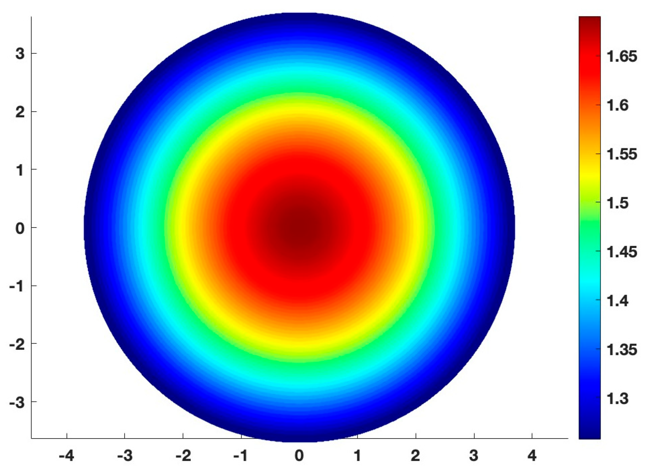
The validation of the 3D-LUNA model is conducted using MATLAB R2023b simulations. In these simulations, the airborne unit operates with a 60-degree beam angle and employs a blue light wavelength. Various parameters in the system are susceptible to errors, primarily due to instrumentation inaccuracies and environmental factors. Key aspects such as transmission power, the altitude of the airborne unit, and the depth of the underwater node are all influenced by measurement uncertainties, which ultimately affect light intensity, as described in Equation (1). In practice, these errors can be significantly minimized through proper calibration and the use of high-precision sensors. For the simulations, we assume that errors in measurable parameters follow a Gaussian distribution with a zero mean and a standard deviation of 1%. Additionally, the position of the underwater node is estimated using an inertial navigation system (INS), which introduces its own errors due to spatial and angular displacement. These errors are also modeled as Gaussian with a zero mean and a 1% standard deviation. The underwater environment is simulated as pure seawater with an extinction coefficient of 0.056.
In our previous work [
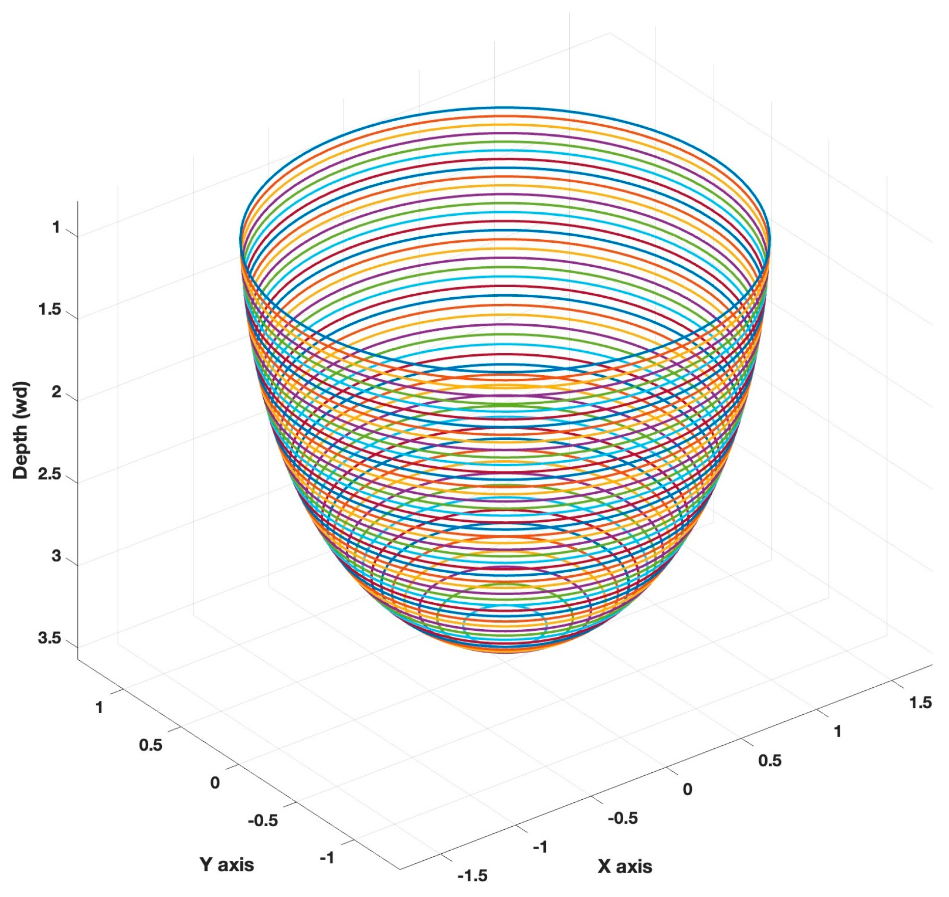
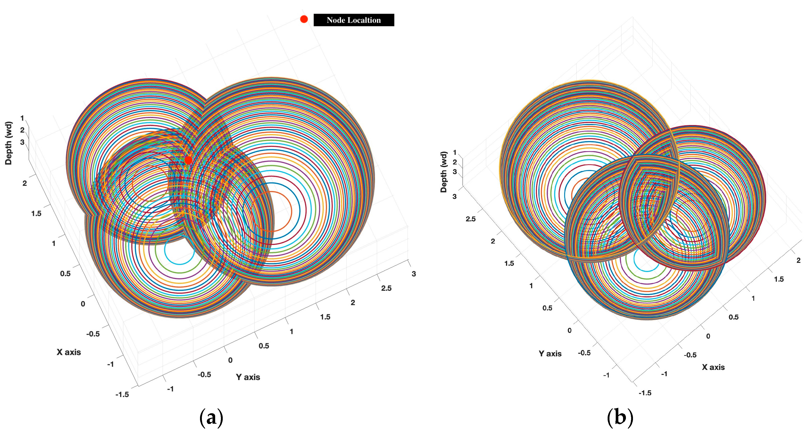
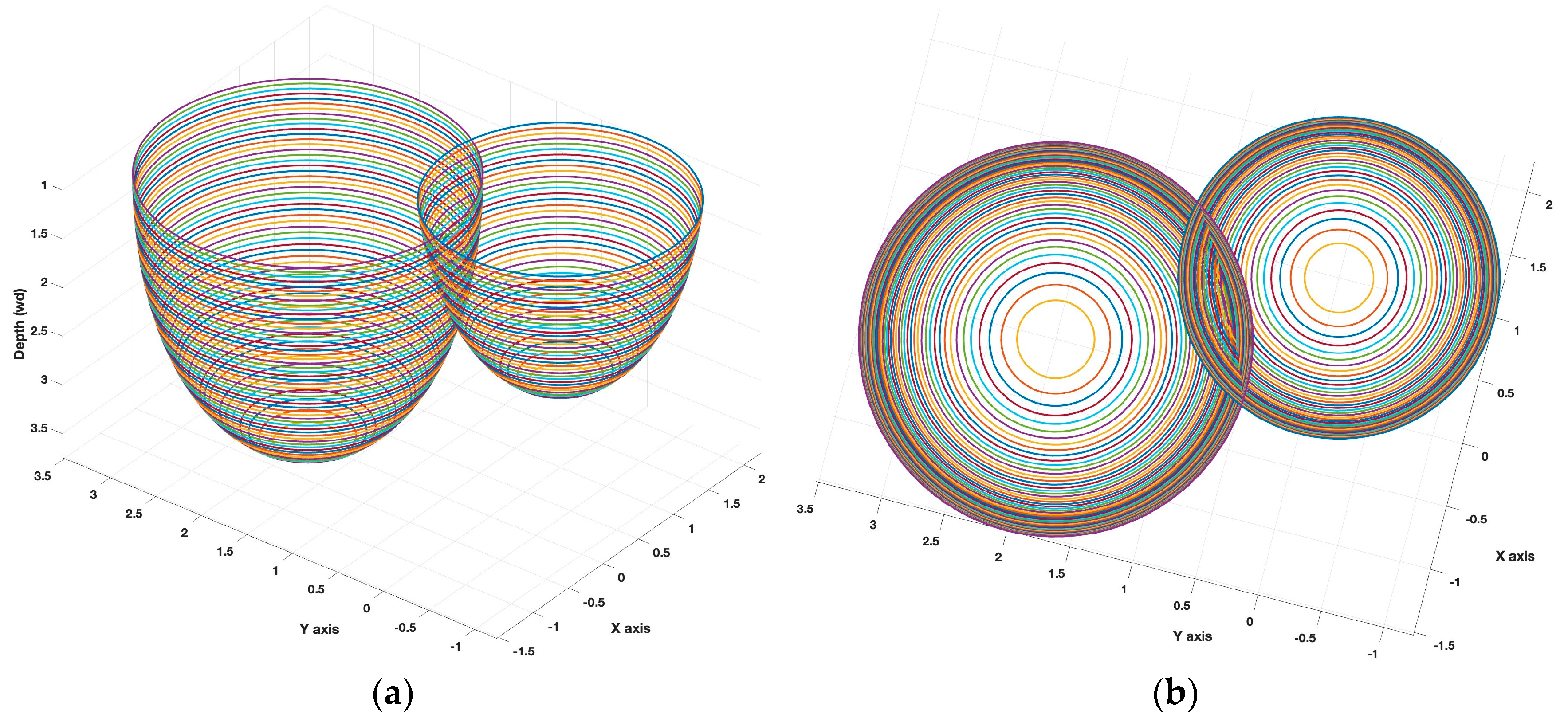
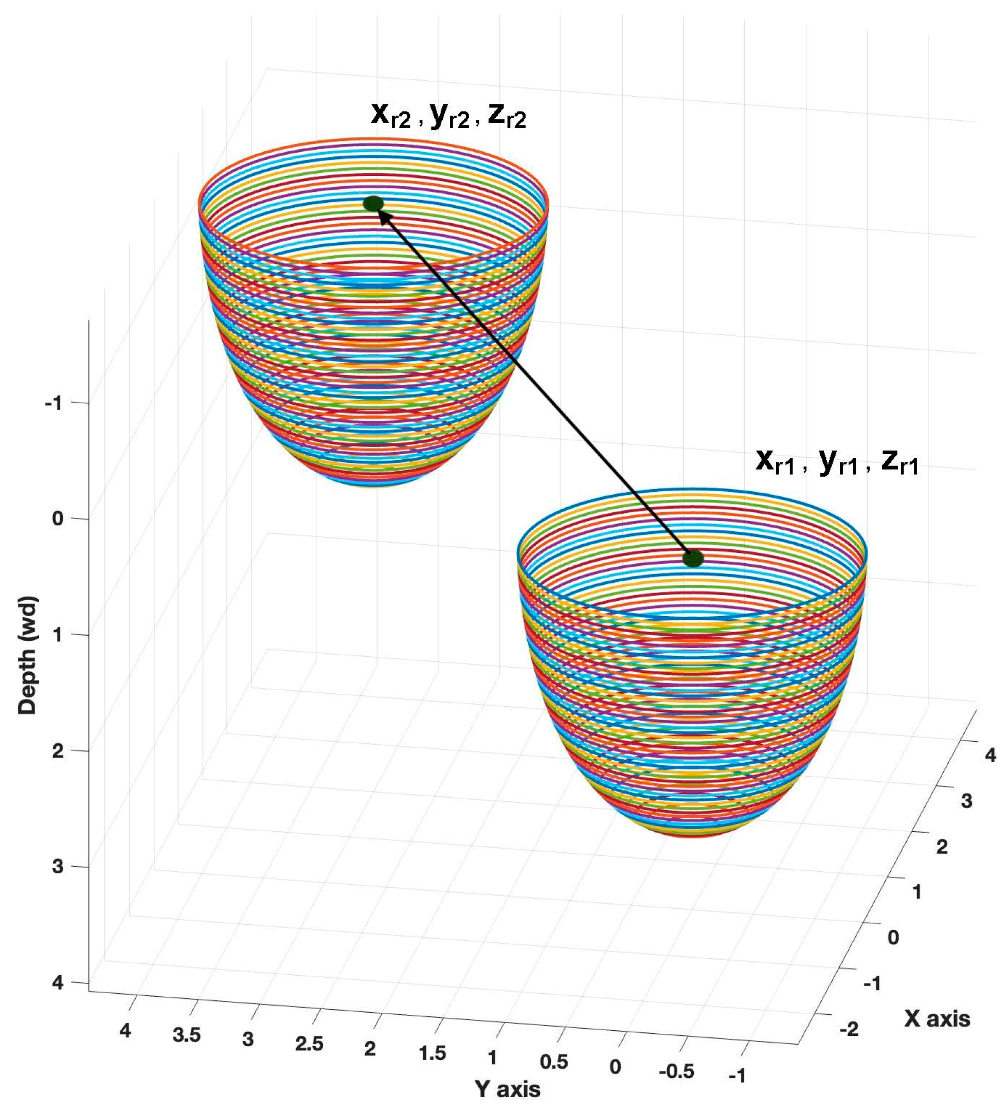
5], we investigated underwater node localizability while considering the mobility patterns of both airborne and underwater nodes. The key aspect is whether the underwater nodes receive sufficient transmissions for accurate localization. In this study, we focus on the localization error of nodes that do not know their underwater depth and receive an adequate number of transmissions. To evaluate the localization performance of 3D-LUNA, we consider a deployment region of 100 m × 100 m × 10 m, which is divided into 100 equal-sized cells. Given the unique characteristics of this localization approach, we compare its performance against an alternative VLC-based localization model, which we refer to as OMNI. In the OMNI model, an underwater VLC transmitter is located at the center of each cell. Specifically, each cell is a 10 m cube where the transmitter is positioned at the center, emitting light omni-directionally. The underwater target node, upon receiving and measuring the light intensity, estimates its location using an inverse square law using underwater attenuation, i.e., using the following:
I = P 4 π w d 1 2   e k w d 1
Though 3D-LUNA modality only deals with directional transmission, it still covers an entire cell since the VLC source is airborne. Omni-directionality is necessary for an underwater light source to cover the entire cell to ensure localizability under the OMNI method (OMNI does not have to handle cross-medium transmission since it is transmitting from underwater). This comparative analysis aims to assess the accuracy and reliability of 3D-LUNA in underwater localization scenarios.

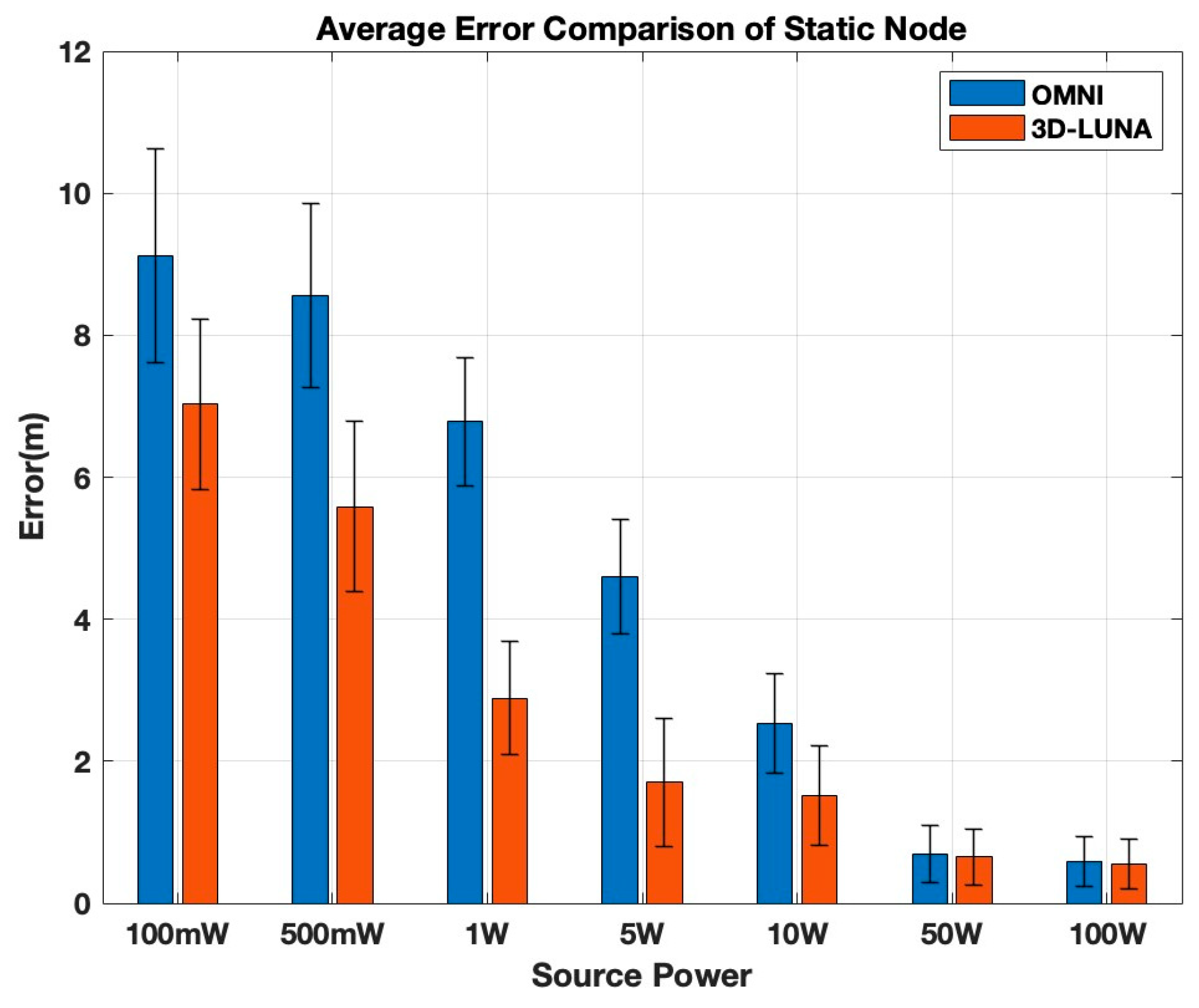
5.1. Stationary Node

For stationary underwater nodes, 30 nodes are placed underwater in random locations. We then compare the performance of both OMNI and 3D-LUNA. Figure 8 shows the localization error for both methods under varying transmission power. The results reflect the average of 100 iterations.
As indicated by the results, 3D-LUNA consistently outperforms Omni by maintaining a lower localization error across all power levels. At low power levels (100 mW–1 W), Omni’s error is significantly higher compared to 3D-LUNA, with the gap remaining noticeable at 500 mW and 1 W. In the mid-power range (5 W–10 W), Omni still exhibits nearly double the error of 3D-LUNA at 5 W, though the difference starts to shrink at 10 W. However, at higher power levels (50 W and 100 W), both methods achieve similar accuracy, with error becoming minimal, indicating that at very high power, transmission strength dominates over method choice. When analyzing the error rate change relative to power levels, 3D-LUNA clearly stands out as it consistently demonstrates a higher reduction rate at lower power levels, particularly between 100 mW and 5 W. Initially, between 100 mW and 500 mW, 3D-LUNA achieves an error reduction rate of approximately 15–20%, whereas OMNI reduces error by only 10–15%. As power increases to 1 W, the gap widens, with 3D-LUNA achieving up to 30–35% reduction compared to OMNI’s 20–25%. The most significant divergence occurs between 1 W and 5 W, where 3D-LUNA reaches a peak reduction of 50–55%, nearly 10–15% higher than OMNI’s 30–40%. This indicates that 3D-LUNA adapts more efficiently in the mid-power range. However, beyond 10 W, both methods experience a sharp decline in rate change, with OMNI dropping to 25–30% and 3D-LUNA maintaining a slight lead at 35–40%. At 50 W and 100 W, both methods exhibit minimal rate change, converging at 5–10%, showing diminishing returns. Overall, the gap in rate change between the two methods is most prominent in the lower-to-mid power range, whereas at high power levels, their performance stabilizes, indicating that 3D-LUNA is most beneficial in power-constrained environments, while both methods perform similarly at high power.
Both OMNI and 3D-LUNA are highly dependent on the transmission power and how the signal intensity is distributed. At lower power levels (100 mW to 5 W), the error is significantly higher for both methods due to weaker signals, which are more susceptible to attenuation and environmental noise. However, the error in OMNI remains consistently larger compared to 3D-LUNA because OMNI distributes power uniformly in all directions, leading to greater signal dispersion and reduced signal strength at the receiver. In contrast, 3D-LUNA appears to use a more concentrated and efficient power distribution, ensuring stronger signal reception and reduced localization error. When power increases beyond 5 W, the stronger transmission mitigates attenuation effects. However, beyond 10 W, both methods approach a point where increasing power has minimal impact on localization error. By 50 W and 100 W, both OMNI and 3D-LUNA reach similar low-error performance, indicating that at these high power levels, the effectiveness of signal distribution becomes less critical as the primary constraints shift to environmental factors. This suggests that while transmission power plays a key role in reducing localization error, the way the power is distributed is crucial at lower power levels, where a more focused transmission like 3D-LUNA provides a significant advantage.
Overall, 3D-LUNA proves to be the superior approach, especially at lower and mid-power levels, offering better accuracy without requiring excessive power, making it a more efficient option in scenarios where power consumption matters.
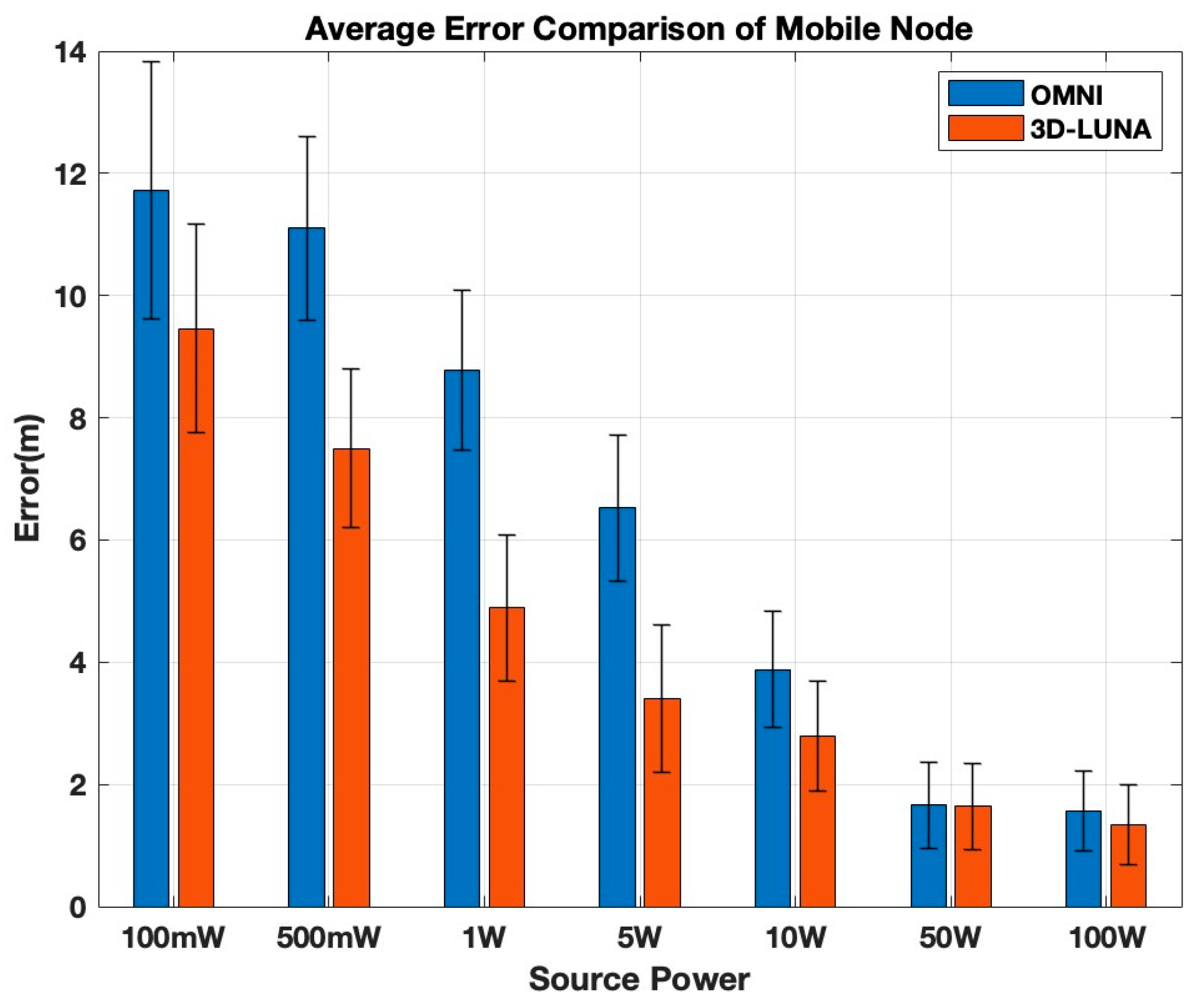
5.2. Mobile Node

To evaluate the localization performance for mobile underwater nodes, we have implemented the random waypoint (RWP) mobility model [40] to simulate the relatively complex movement of the mobile underwater node. In this mobility model, the underwater node moves at a constant speed, beginning its journey from a randomly chosen point within a 3D space. It then travels in a randomly selected direction within the defined region. After a randomly determined duration in the range of 10 to 30 s, the mobile underwater node changes direction, selecting a new random path. Notably, there is no pause time when the mobile underwater node alters its direction. Figure 9 shows the average localization performance for varying transmission power for 100 iterations where a node receives the required number of transmissions to localize itself.
For the mobile node, the comparison between OMNI and 3D-LUNA follows a similar trend to the static node, with 3D-LUNA consistently outperforming OMNI by producing lower localization errors across all power levels. At low power levels (100 mW–1 W), OMNI shows significantly higher errors, reaching approximately 12 m at 100 mW, while 3D-LUNA reduces it to around 10 m. The error remains noticeably higher for OMNI at 500 mW and 1 W, but both methods show a clear improvement as power increases. In the mid-power range (5 W–10 W), OMNI’s error remains significantly higher than 3D-LUNA, though the gap starts to shrink. At higher power levels (50 W–100 W), both methods converge to a similar accuracy level with minimal error, demonstrating that at very high power, the method selection becomes less critical. Overall, 3D-LUNA is a better choice, particularly at lower and mid-power levels, as it ensures greater accuracy without requiring excessive power.
The error rate between consecutive power levels varies for OMNI and 3D-LUNA, but it displays a similar trend to static nodes, with 3D-LUNA consistently outperforming OMNI at lower power levels (100 mW–10 W) due to its more efficient signal distribution. The most significant reduction occurs between 1 W and 5 W, where 3D-LUNA achieves nearly 50% error reduction compared to OMNI’s 30–40%, highlighting its superior power utilization. As power increases to 10 W, the gap narrows, with OMNI beginning to catch up, though 3D-LUNA still maintains a slight advantage (~5–10% more error reduction). Beyond 10 W, and especially from 50 W to 100 W, both methods experience a similar trend, with error reduction rates converging as the power of transmission becomes the dominant factor. This trend suggests that while power distribution optimization is critical at lower power levels, at higher power, the influence of transmission power makes OMNI and 3D-LUNA nearly equivalent in performance.
When comparing static and mobile nodes, the mobile node generally exhibits higher errors across all power levels, indicating that mobility introduces additional localization challenges. At low power levels, the error for mobile nodes is higher than that of static nodes, suggesting that movement increases uncertainty in localization. However, the error reduction pattern remains similar, where higher power levels improve accuracy for both cases, and 3D-LUNA consistently outperforms OMNI. Notably, at high power (50 W and 100 W), the errors in both static and mobile cases converge, showing minimal difference between OMNI and 3D-LUNA, reinforcing the conclusion that transmission power dominates over method selection at these levels. In summary, while both cases benefit from higher power, 3D-LUNA is the superior choice, especially in mobile scenarios where errors tend to be more pronounced.

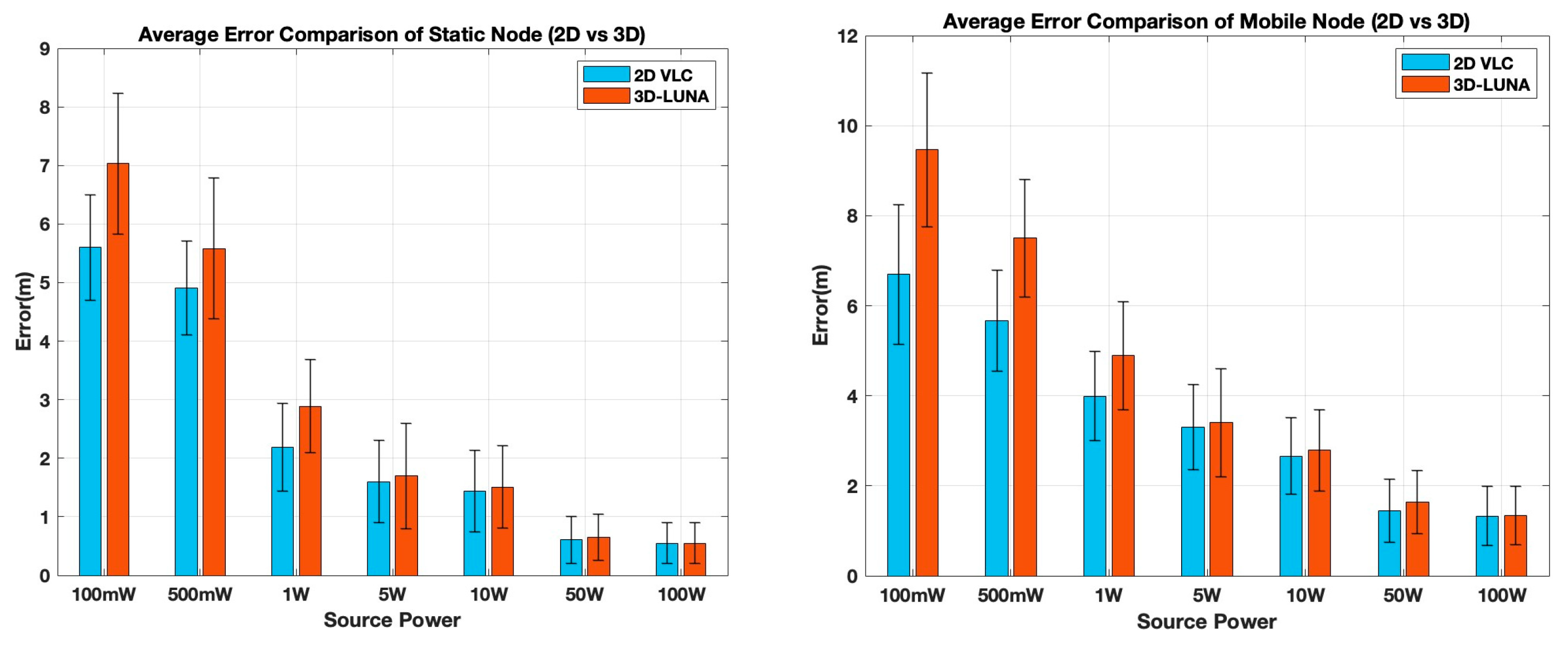
5.3. Two- vs. Three-Dimensional Localization Comparison

We have also compared 3D-LUNA performance with our previous work, which utilizes a depth sensor to convert the localization scheme into a 2D problem for both static [4] and mobile [5] nodes. In both 3D and 2D modality, the transmission scheme is exactly the same, but 3D-LUNA does not require the depth information acquired from the depth sensor. Figure 10 shows a comparison of performance for both static and mobile modality.
For static nodes, the results show that both methods experience higher localization errors at lower power levels (100 mW and 500 mW), with 3D-LUNA exhibiting higher errors than 2D VLC. This is expected, as 2D VLC benefits from an external depth measurement, improving its localization accuracy in weaker signal conditions. However, as the source power increases, the errors for both methods progressively and significantly decrease, and beyond 10 W, the difference between 2D VLC and 3D-LUNA becomes negligible. At 50 W and 100 W, both approaches yield nearly identical performance, demonstrating that 3D-LUNA can achieve similar accuracy without relying on a pressure sensor when sufficient power is available. This is a significant advantage, as it eliminates the dependency on external sensors, making 3D-LUNA a more autonomous and hardware-efficient solution.
For mobile nodes, a similar trend is observed, but with generally higher errors compared to static nodes, emphasizing the challenges introduced by movement. At lower power levels, 2D VLC again has an advantage, as the depth information from the pressure sensor provides a more stable reference. However, as power levels increase, the error difference between 2D VLC and 3D-LUNA shrinks, and by 50 W and 100 W, their performances are nearly indistinguishable. The error bars also indicate that the variability in localization accuracy decreases with increasing power, making high-power scenarios more reliable for both methods.
The most critical takeaway from this analysis is that while 2D VLC gains an initial advantage by incorporating a pressure sensor, 3D-LUNA ultimately achieves comparable localization accuracy without requiring any additional hardware. This makes 3D-LUNA a more flexible and practical solution, particularly in environments where sensor failures, calibration issues, or additional hardware costs are of concern. By eliminating the need for pressure sensors while maintaining accuracy at moderate-to-high power levels, 3D-LUNA offers a scalable and efficient approach to localization, making it a strong candidate for real-world deployment in both static and mobile scenarios.

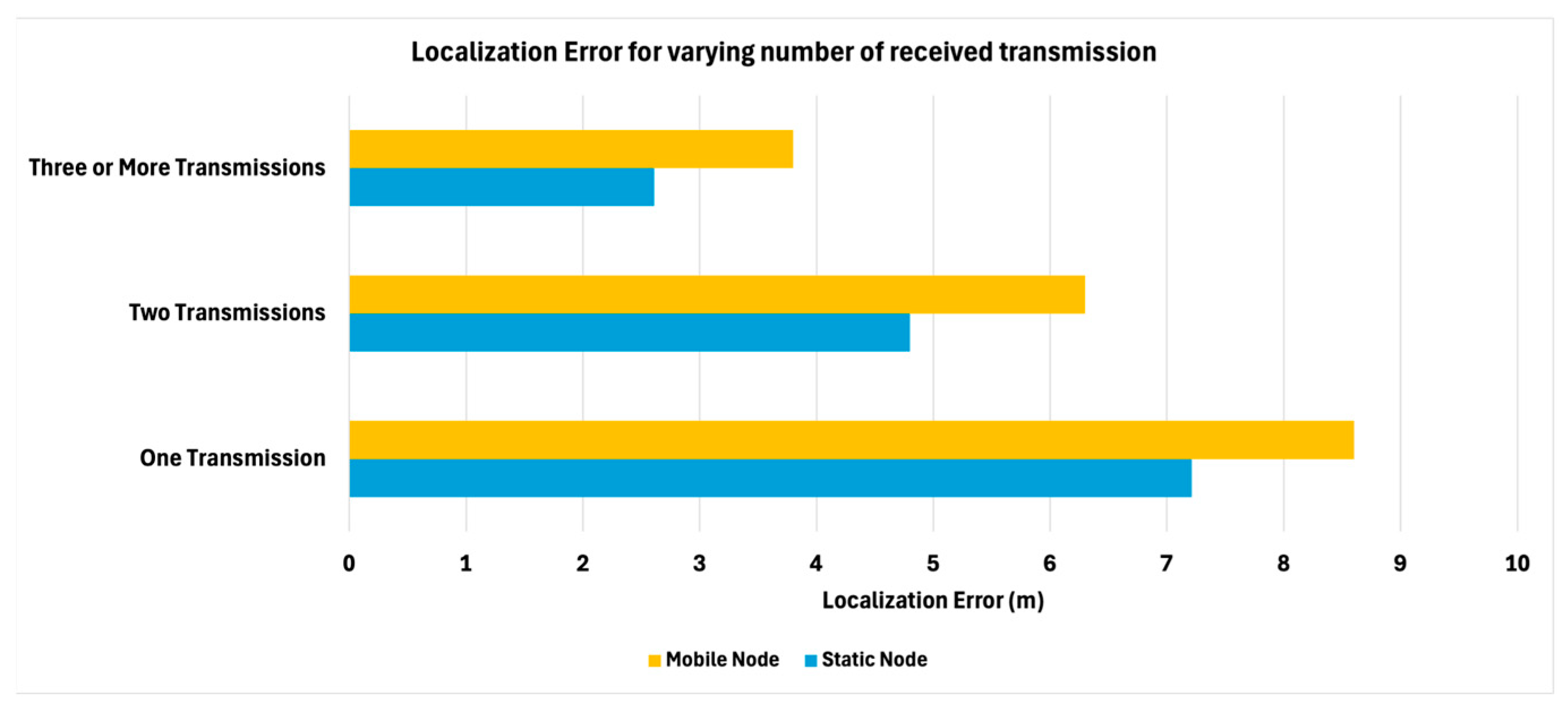
5.4. Number of Received Transmissions

We have also investigated how the number of received transmissions affects the accuracy of 3D-LUNA for both static and mobile nodes using a fixed transmission power (10 W).
In Figure 11, the results indicate that localization error decreases as the number of received transmissions increases for both node types. When only one transmission is received, the mobile node exhibits the highest error, whereas the static node shows a slightly lower error. With two transmissions, the localization error improves for both cases. The best accuracy is achieved when three or more transmissions are received, where the mobile node’s error is around 4 m, and the static node demonstrates the least error.

6. Conclusions

This paper presents 3D-LUNA, a novel approach for 3D localization of underwater nodes using airborne VLC beams. By leveraging the intensity of light received by submerged nodes, 3D-LUNA eliminates the need for surface-based reference points, making it a viable solution for stealth-sensitive applications such as military operations, environmental monitoring, and underwater exploration. Simulation results confirm that 3D-LUNA achieves superior accuracy compared to omni-directional VLC methods, particularly when depth information is unavailable. The method remains effective across a range of transmission powers and demonstrates adaptability to both stationary and mobile underwater nodes. Additionally, the proposed error mitigation strategies improve localization robustness under uncertain measurement conditions. The results presented in this work demonstrate the potential of 3D-LUNA as a reliable and infrastructure-free localization framework for underwater environments. Compared to traditional acoustic-based localization methods, which often report localization errors ranging from 1.5 to 5 m under similar simulation conditions, 3D-LUNA consistently achieves sub-meter accuracy, often within 0.3 to 0.7 m, depending on beam configuration.
As part of future work, we intend to extend the 3D-LUNA framework in several key directions. First, we plan to incorporate learning-based techniques to enhance localization robustness under highly dynamic and optically heterogeneous underwater conditions. We also aim to refine the physical modeling by accounting for complex aquatic phenomena such as surface-wave-induced refraction, turbidity variations, and thermocline effects. In addition, we seek to validate the proposed approach through experimental testing in real or controlled underwater environments.

Author Contributions

Conceptualization, J.B.S. and M.Y.; methodology, J.B.S. and M.Y.; validation, J.B.S., M.Y. and F.-S.C.; formal analysis, J.B.S. and M.Y.; investigation, J.B.S., M.Y. and F.-S.C.; writing—original draft preparation, J.B.S. and M.Y.; writing—review and editing, J.B.S., M.Y. and F.-S.C.; visualization, J.B.S. and M.Y.; supervision, M.Y. and F.-S.C.; project administration, M.Y. and F.-S.C.; funding acquisition, M.Y. and F.-S.C. All authors have read and agreed to the published version of the manuscript.

Funding

This work is supported by the National Science Foundation, USA, Contract #0000010465.

Institutional Review Board Statement

Not applicable.

Informed Consent Statement

Not applicable.

Data Availability Statement

Data are contained within the article.

Conflicts of Interest

The authors declare no conflict of interest.

References

  1. Ullah, I.; Chen, J.; Su, X.; Esposito, C.; Choi, C. Localization and Detection of Targets in Underwater Wireless Sensor Using Distance and Angle Based Algorithms. IEEE Access 2019, 7, 45693–45704. [Google Scholar] [CrossRef]
  2. Zhang, L.; Zhang, T.; Shin, H.-S.; Xu, X. Efficient Underwater Acoustical Localization Method Based on Time Difference and Bearing Measurements. IEEE Trans. Instrum. Meas. 2021, 70, 8501316. [Google Scholar] [CrossRef]
  3. Available online: https://www.msn.com/en-ca/news/world/russia-s-covert-underwater-operations-challenge-uk-security/ar-AA1CoTO3 (accessed on 29 April 2025).
  4. Mahmud, M.; Islam, M.S.; Ahmed, A.; Younis, M.; Choa, F.-S. Cross-Medium Photoacoustic Communications: Challenges, and State of the Art. Sensors 2022, 22, 4224. [Google Scholar] [CrossRef] [PubMed]
  5. N’doye, I.; Zhang, D.; Alouini, M.-S.; Laleg-Kirati, T.-M. Establishing and Maintaining a Reliable Optical Wireless Communication in Underwater Environment. IEEE Access 2021, 9, 62519–62531. [Google Scholar] [CrossRef]
  6. Saif, J.B.; Younis, M. Underwater Localization using Airborne Visible Light Communication Links. In Proceedings of the IEEE Global Communications Conference (GLOBECOM), Madrid, Spain, 7–11 December 2021; pp. 1–6. [Google Scholar]
  7. Saif, J.B.; Younis, M.; Choa, F.-S.; Ahmed, A. Localization of Autonomous Underwater Vehicles using Airborne Visible Light Communication Links. In Proceedings of the 32nd Wireless and Optical Communications Conference (WOCC), Newark, NJ, USA, 5–6 May 2023; pp. 1–6. [Google Scholar]
  8. Saif, J.B.; Younis, M.; Choa, F.-S.; Ahmed, A. Global Positioning of Underwater Nodes Using Airborne-Formed Visual Light Beams and Acoustic Ranging. In Proceedings of the IEEE International Conference on Communications (ICC), Denver, CO, USA, 9–13 June 2024; pp. 4239–4244. [Google Scholar]
  9. Lin, S.; An, J.; Gan, L.; Debbah, M. UAV-Mounted SIM: A Hybrid Optical-Electronic Neural Network for DoA Estimation. In Proceedings of the ICASSP 2025—IEEE International Conference on Acoustics, Speech and Signal Processing, Hyderabad, India, 6–11 April 2025. [Google Scholar]
  10. Dong, M.; Li, H.; Qin, Y.; Hu, Y.; Huang, H. A Secure and Accurate Localization Algorithm for Mobile Nodes in Underwater Acoustic Network. Eng. Appl. Artif. Intell. 2024, 133 Pt B, 108157. [Google Scholar] [CrossRef]
  11. Jiang, Y.; Renner, B.-C. Low-Cost Underwater Swarm Acoustic Localization: A Review. IEEE Access 2024, 12, 25779–25796. [Google Scholar] [CrossRef]
  12. Zhao, D.-D.; Mao, W.-B.; Chen, P.; Dang, Y.-J.; Liang, R.-H. FPGA-Based Real-Time Synchronous Parallel System for Underwater Acoustic Positioning and Navigation. IEEE Trans. Ind. Electron. 2024, 71, 3199–3207. [Google Scholar] [CrossRef]
  13. Alahmad, R.; Alraie, H.; Hasaba, R.; Eguchi, K.; Matsushima, T.; Fukumoto, Y.; Ishii, K. Performance Analysis of Underwater Radiofrequency Communication in Seawater: An Experimental Study. J. Mar. Sci. Eng. 2024, 12, 2104. [Google Scholar] [CrossRef]
  14. Qu, Z.; Lai, M. A Review on Electromagnetic, Acoustic, and New Emerging Technologies for Submarine Communication. IEEE Access 2024, 12, 12110–12125. [Google Scholar] [CrossRef]
  15. Hansen, R.C. Fundamental Limitations in Antennas. Proc. IEEE 1981, 69, 170–182. [Google Scholar] [CrossRef]
  16. Oh, J.; Yoon, K.; Lee, H.J.; Kim, J.-Y.; Cho, I.-K. Magnetic Induction (MI)-Based Wireless Communication for Challenging Environments. In Proceedings of the IEEE Asia-Pacific Microwave Conference (APMC), Bali, Indonesia, 17–20 November 2024; pp. 1–3. [Google Scholar]
  17. Xu, S.; Zhu, B.; Wu, X.; Doğançay, K. Optimal TOA-Based Sensor-Anchor-Source Geometries and Estimation Bounds for Simultaneous Sensor and Source Localization. IEEE Trans. Signal Process. 2025, in press. [CrossRef]
  18. Rezzouki, M.; Ferré, G.; Terrasson, G.; Llaria, A. Net Fishing Localization: Performance of TDOA-Based Positioning Technique in Underwater Acoustic Channels Using Chirp Signals. In Proceedings of the IEEE ISCAS, Singapore, 19–22 May 2024; pp. 1–5. [Google Scholar]
  19. Huang, H.; Zheng, Y.R. AoA Assisted Localization for Underwater Ad-Hoc Sensor Networks. In Proceedings of the OCEANS 2016 MTS/IEEE, Monterey, CA, USA, 19–23 September 2016; pp. 1–6. [Google Scholar]
  20. Nguyen, T.L.N.; Shin, Y. An Efficient RSS Localization for Underwater Wireless Sensor Networks. Sensors 2019, 19, 3105. [Google Scholar] [CrossRef]
  21. Schmidt, R.O. Multiple Emitter Location and Signal Parameter Estimation. Adapt. Antennas Wirel. Commun. 2009, 34, 190–194. [Google Scholar] [CrossRef]
  22. Huang, H.; Zheng, Y.R. Node Localization with AoA Assistance in Multi-Hop Underwater Sensor Networks. Ad Hoc Netw. 2018, 78, 32–41. [Google Scholar] [CrossRef]
  23. Zhou, Y.; He, J.; Chen, K.; Chen, J.; Liang, A. An Area Localization Scheme for Large Scale Underwater Wireless Sensor Networks. In Proceedings of the WRI International Conference on Communications and Mobile Computing, Kunming, China, 6–8 January 2009; pp. 543–547. [Google Scholar]
  24. Lee, S.; Kim, K. Localization with a Mobile Beacon in Underwater Acoustic Sensor Networks. Sensors 2012, 12, 5486–5501. [Google Scholar] [CrossRef]
  25. Han, Y.; Zheng, C.; Sun, D. Accurate Underwater Localization Using LBL Positioning System. In Proceedings of the OCEANS 2015 MTS/IEEE, Washington, DC, USA, 19–22 October 2015; pp. 1–4. [Google Scholar]
  26. Cario, G.; Casavola, A.; Gagliardi, G.; Lupia, M.; Severino, U. Accurate Localization in Acoustic Underwater Localization Systems. Sensors 2021, 21, 762. [Google Scholar] [CrossRef]
  27. Reis, J.; Morgado, M.; Batista, P.; Oliveira, P.; Silvestre, C. Design and Experimental Validation of a USBL Underwater Acoustic Positioning System. Sensors 2016, 16, 1491. [Google Scholar] [CrossRef]
  28. Li, N.; Martínez, J.-F.; Meneses Chaus, J.; Eckert, M. A Survey on Underwater Acoustic Sensor Network Routing Protocols. Sensors 2016, 16, 414. [Google Scholar] [CrossRef]
  29. Gong, Z.; Li, C.; Su, R. Fundamental Limits of Doppler Shift-Based, ToA-Based, and TDoA-Based Underwater Localization. IEEE/CAA J. Autom. Sin. 2023, 10, 1637–1639. [Google Scholar]
  30. Lin, C.; Yu, Y.; Xiong, J.; Zhang, Y.; Wang, L.; Wu, G.; Luo, Z. Shrimp: A Robust Underwater Visible Light Communication System. In Proceedings of the ACM MobiCom, New Orleans, LA, USA, 25–29 October 2021; pp. 134–146. [Google Scholar]
  31. Elamassie, M.; Miramirkhani, F.; Uysal, M. Performance Characterization of Underwater Visible Light Communication. IEEE Trans. Commun. 2019, 67, 543–552. [Google Scholar] [CrossRef]
  32. Islam, M.S.; Younis, M.F. Analyzing Visible Light Communication Through Air–Water Interface. IEEE Access 2019, 7, 123830–123845. [Google Scholar] [CrossRef]
  33. Fang, C.; Li, S.; Wang, Y.; Wang, K. High-Speed Underwater Optical Wireless Communication with Advanced Signal Processing Methods Survey. Photonics 2023, 10, 811. [Google Scholar] [CrossRef]
  34. Elfikky, A.; Boghdady, A.I.; Mumtaz, S.; Elsayed, E.E.; Singh, M.; Abd El-Mottaleb, S.A.; Mohsan, S.A.H.; Aly, M.H. Underwater Visible Light Communication: Recent Advancements and Channel Modeling. Opt. Quant. Electron. 2024, 56, 1617. [Google Scholar] [CrossRef]
  35. Carver, C.J.; Shao, Q.; Lensgraf, S.; Sniffen, A.; Perroni-Scharf, M.; Gallant, H.; Li, A.Q.; Zhou, X. Sunflower: Locating Underwater Robots from the Air. In Proceedings of the ACM MobiSys, Portland, Oregon, 27 June–1 July 2022; pp. 14–27. [Google Scholar]
  36. Mahmud, M.; Younis, M.; Carter, G.; Choa, F.-S. Underwater Node Localization Using Optoacoustic Signals. In Proceedings of the IEEE International Conference on Communications (ICC), Seoul, Republic of Korea, 16–20 May 2022; pp. 4444–4449. [Google Scholar]
  37. Islam, M.S.; Younis, M.; Mahmud, M.; Choa, F.-S. An Efficient Pulse Position Modulation Scheme to Improve the Bit Rate of Photoacoustic Communication. In Proceedings of the 32nd Wireless and Optical Communications Conference (WOCC), Newark, NJ, USA, 5–6 May 2023; pp. 1–6. [Google Scholar]
  38. Bai, X.; Liang, Z.; Zhu, Z.; Schwing, A.; Forsyth, D.; Gruev, V. Polarization-Based Underwater Geolocalization with Deep Learning. eLight 2023, 3, 15. [Google Scholar] [CrossRef]
  39. Santos, M.M.D.; De Giacomo, G.G.; Drews-Jr, P.L.J.; Botelho, S.S.C. Cross-View and Cross-Domain Underwater Localization Based on Optical Aerial and Acoustic Underwater Images. IEEE Robot. Autom. Lett. 2022, 7, 4969–4974. [Google Scholar] [CrossRef]
  40. Hyytiä, E.; Virtamo, J. Random Waypoint Mobility Model in Cellular Networks. Wirel. Netw. 2007, 13, 177–188. [Google Scholar] [CrossRef]
Figure 1. A 2D illustration of the coverage of light transmission from a source at S above the water surface. The points A, B, C, F, G, H, and J are geometric points of reference.
Photonics 12 00503 g001
Figure 2. Plotting the distribution of light intensity and the associated underwater coverage for an airborne VLC beam that is normal to the water surface.
Photonics 12 00503 g002
Figure 3. Location estimation of an underwater node using airborne VLC beam intensity in the absence of depth information.
Photonics 12 00503 g003
Figure 4. The scenario of receiving three transmissions. (a) Bottom view; (b) top view.
Photonics 12 00503 g004
Figure 5. The scenario when only transmissions are received: (a) 3D view; (b) top view.
Photonics 12 00503 g005
Figure 6. Location projection due to the underwater node mobility.
Photonics 12 00503 g006
Figure 7. Flowchart illustrating the centroid computation process based on VLC transmission reception and shape intersection analysis.
Photonics 12 00503 g007
Figure 8. Localization performance comparison between 3D-LUNA and OMNI for static nodes. The error bars represent 95% confidence intervals.
Photonics 12 00503 g008
Figure 9. Localization performance comparison between 3D-LUNA and OMNI for mobile nodes. The error bars represent 95% confidence intervals.
Photonics 12 00503 g009
Figure 10. Localization performance comparison between 2D VLC and 3D-LUNA for static and mobile nodes. The error bars represent 95% confidence intervals.
Photonics 12 00503 g010
Figure 11. Localization performance comparison for varying numbers of transmissions.
Photonics 12 00503 g011
Table 1. Definition of the notation used.
NotationDescription
P Power of the light source
θ Beam angle of the light source for a flat surface
θ i Incident angle of water surface for a flat surface
θ r Refraction angle for a flat surface
a d Distance of light source from water surface for a flat surface
w d Depth of the sensor from water surface for a flat surface
η Reflectance of light
τ Transmittance of light
SAirborne transmitter position
Disclaimer/Publisher’s Note: The statements, opinions and data contained in all publications are solely those of the individual author(s) and contributor(s) and not of MDPI and/or the editor(s). MDPI and/or the editor(s) disclaim responsibility for any injury to people or property resulting from any ideas, methods, instructions or products referred to in the content.

