Non-Iterative Phase-Only Hologram Generation via Stochastic Gradient Descent Optimization

Abstract

In this work, we explored, for the first time, to the best of our knowledge, the potential of stochastic gradient descent (SGD) to optimize random phase functions for application in non-iterative phase-only hologram generation. We defined and evaluated four loss functions based on common image quality metrics and compared the performance of SGD-optimized random phases with those generated using Gerchberg–Saxton (GS) optimization. The quality of the reconstructed holograms was assessed through numerical simulations, considering both accuracy and computational efficiency. Our results demonstrate that SGD-based optimization can produce higher-quality phase holograms for low-contrast target scenes and presents nearly identical performance to GS-optimized random phases for high-contrast targets. Experimental validation confirmed the practical feasibility of the proposed method and its potential as a flexible alternative to conventional GS-based optimization.

1. Introduction

Computer-generated holography (CGH) has become an essential technique in modern applications, including optical trapping [1,2], optogenetics [3,4], microscopy [5,6], and holographic displays [7,8]. This is because CGH, when combined with modern spatial light modulator (SLM) setups, enables precise control of both the amplitude and phase of a light field in three-dimensional (3D) space.

Despite these advantages, current CGH applications still face significant limitations. High-quality CGH generation relies on computationally demanding iterative algorithms, which make real-time processing challenging in standard computing hardware. Additionally, for applications that use CGH in conjunction with SLMs, the characteristics of these devices must be considered when designing CGH methods.

SLMs are typically capable of either phase-only or amplitude-only modulation, with phase-only modulation being preferred due to its higher diffraction efficiency [9]. As a result, CGH algorithms must encode target fields into phase-only holograms (POHs). However, no general exact solution exists for this, leading to the development of numerous POH generation algorithms tailored to different target field characteristics, accuracy requirements, and computational constraints.

One of the earliest approaches to generating phase holograms was the Gerchberg–Saxton (GS) algorithm [9]. This iterative method determines the phase that connects the hologram and its Fourier plane by imposing an amplitude constraint on the hologram plane. A Fourier transform is then applied, and the resulting amplitude is replaced by the target amplitude. This process is repeated iteratively until a suitable approximation of the target amplitude is obtained in the Fourier domain. However, the basic GS algorithm is limited to generating Fourier holograms of two-dimensional (2D) amplitude objects and exhibits relatively low accuracy.

Numerous variants of the GS algorithm have been developed to extend the capabilities of the original method, including adaptations for Fresnel holograms [10], multiplane scenes [11], and improved convergence constraints [12]. However, high-resolution and high-accuracy holograms often require significant computation time.

Another technique broadly used in CGH is error diffusion. Originally developed to reduce the quantization noise introduced by binarizing an amplitude-only or phase-only hologram, this method involves calculating the difference in value between a pixel before binarization and after the process. This difference in value, called error, is then distributed to the neighboring pixels using specific weight factors. This process is repeated for all pixels in the hologram. The result is a binary phase-only or amplitude-only hologram, capable of reproducing a scene with reduced binarization noise [13]. This approach has certain limitations: since all pixels must be updated sequentially, the error diffusion computation can be very slow for high-resolution holograms. Moreover, while noise is reduced for low-frequency components, it remains significant in the high frequencies of the reconstruction, thereby limiting the effective bandwidth of the scene. Error diffusion is not restricted to hologram binarization and has been used to convert complex holograms into phase-only functions [14] or to encode band-limited color scenes into a single-phase hologram [15].

More recently, phase CGH methods based on stochastic gradient descent (SGD) [16,17,18,19] and other optimization techniques have attracted interest. These methods define a loss function to measure the similarity between the target field and the field generated by a POH and then optimize the hologram to minimize this loss function. Unlike GS-based methods, optimization approaches offer greater flexibility, enabling the generation of phase-only, amplitude-only, or complex-valued holograms. Loss functions can be customized to enhance the specific characteristics of the target field, thereby enabling their application in a wide range of scenarios [20]. Additionally, unlike conventional GS, SGD approaches can be used to generate Fourier or Fresnel holograms of any type of scene, including 2D, 3D, or multiplane ones [21]. However, these methods require computing the gradient of the loss function at each iteration, which can be computationally intensive. This often necessitates advanced mathematical techniques, such as Wirtinger calculus [17], making SGD-based hologram generation even more demanding than GS-based methods and, therefore, unsuitable for real-time applications.

Due to the computational challenges of iterative methods like GS and SGD, there is increasing interest in non-iterative approaches for phase hologram generation. Although these methods generally offer reduced accuracy, they present a substantial advantage in terms of computational speed. One notable non-iterative approach is the double-phase hologram technique [22]. This method encodes a complex field into two interleaved phase functions, enabling its reconstruction after suppressing unwanted diffraction orders. However, because the field is encoded into two interleaved phase functions, the effective resolution is halved, which limits the accuracy of the reconstructed field, particularly in experimental setups constrained by the limited resolution of available SLMs. Variants of double-phase holography have been proposed to optimize interleaving patterns [23], to modify the definition of the two phases [24], or to reduce noise by using the spatiotemporal interleaving of multiple phase functions instead of the conventional spatial-only interleaving of two phases [25].

Another non-iterative method is phase tailoring, which involves selecting a phase function where, when combined with the target field, the resulting distribution approximates the desired phase hologram through an inverse transformation. One representative example is the use of random phase functions [26,27]. Although simple to implement, random phase methods introduce significant speckle noise, which reduces the hologram quality.

To address this limitation, patterned random phase techniques have been introduced [28], in which a repeating random phase block is used to improve the reconstruction accuracy. However, this technique introduces undesirable artifacts due to the periodicity of the phase pattern. Another alternative is the use of quadratic phase functions [29], which reduce speckle noise but may lead to ringing artifacts in the reconstructed field.

An improved strategy involves optimizing tailored phase functions using iterative methods. One such method is the optimized random phase (ORAP) approach, where an initial random phase is optimized for a specific resolution, target size, and illumination wavelength using the GS algorithm [30]. Once optimized, the resulting ORAP can be reused to generate phase holograms for multiple target scenes without requiring further iterations. This leads to a substantial enhancement in hologram quality compared with unoptimized random phases. Extensions of this method have been proposed for Fresnel holograms and 3D objects [31]. Similarly, quadratic phase functions optimized using iterative algorithms such as GS have also shown improved performance over their unoptimized counterparts [32].

Despite these advancements, current phase tailoring methods rely on GS-based optimization, which may not be the most effective or flexible approach for optimizing random phase functions. In this context, the potential of SGD-based optimization for non-iterative hologram generation must be explored. Given the demonstrated versatility of SGD in CGH applications, this work aimed to determine whether optimizing random phase functions using SGD can produce phase holograms of comparable or superior quality to those generated using GS-optimized random phases while maintaining computational efficiency. To achieve this, we applied SGD to optimize random phases using four distinct loss functions based on widely used image quality metrics. The resulting holograms were compared with those generated via conventional GS-optimized random phases, evaluating both the reconstruction quality and computational efficiency. Finally, the numerical and experimental results are presented to validate the effectiveness of the proposed approach.

2. Phase Hologram Generation

2.1. Gerchberg–Saxton Algorithm

The most well-known approach to generating phase holograms is the GS algorithm, along with its variations. To generate a phase hologram using the GS algorithm, we first multiply the target amplitude $A_T(x,y)$, whose hologram we want to generate, by an initial phase ${\varphi }_i(x,y)$. Thus, we obtain the initial field in the reconstruction plane, given by

$$F_i(x,y)=A_T(x,y)e^{i{\varphi }_i(x,y)}$$

(1)

Subsequently, an inverse Fourier transform (IFT) is performed to propagate the resulting complex field from the reconstruction plane to the hologram plane.

$$H{\prime }_i(v,w)=IFT\{F_i(x,y\}$$

(2)

Afterward, we replace the amplitude of the resulting field in the hologram plane with a constant value $C$, while its phase is preserved ${\theta }_i(v,w)$.

$$H_i(v,w)=C{e}^{i{\theta }_i(v,w)}$$

(3)

Next, we perform a Fourier transform (FT) from the hologram plane to the reconstruction plane, where the resulting amplitude of the field is replaced by the target amplitude, preserving the phase ${\varphi }_{i+1}(x,y)$.

$$\begin{array}{l}{F}_{i+1}(x,y)=FT\{H_i(v,w)\}\\ F_{i+1}(x,y)=A_T(x,y){\mathrm{e}}^{i{\varphi }_{i+1}(x,y)}\end{array}$$

(4)

This process is repeated iteratively until the reconstructed amplitude sufficiently approximates the target amplitude, or until a predefined computation time limit is reached. The phase in the hologram $H_i(v,w)$ after $i$iterations of the GS algorithm represents the final phase hologram. This approach can produce holograms of relatively high quality but is prone to stagnation.

2.2. Stochastic Gradient Descent Optimization

In their most basic form, SGD phase hologram generation methods [17] consist of finding a phase $\varphi (k,l)$, such that, after a reconstruction process, the loss function $L(\varphi ,A_T)$ is minimized. $A_T(i,j)$ denotes the target amplitude to be encoded in the hologram, $i$ and $j$ are pixel coordinates in the reconstruction plane, and $k$ and $l$ correspond to pixel coordinates in the hologram plane.

In the case analogous to the GS algorithm, if the goal is to obtain the target amplitude after a Fourier transform, the reconstructed amplitude can be defined as

$$R(i,j)=\left|FT(e^{i\varphi (k,l)})\right|$$

(5)

By defining the mean square error (MSE) as a loss function, we have

$$L_{mse}(\varphi ,A_T)={\displaystyle \frac{1}{NM}}{\displaystyle \sum _{i,j}^{N,M}{(R(i,j)-A_T(i,j))}^2}$$

(6)

To minimize this loss using SGD optimization, a first guess for the phase $\varphi (k,l)$ is defined. Then, the gradient of the loss function is computed, and a new phase is obtained with the following equation:

$${\varphi }_{n+1}(k,l)={\varphi }_n(k,l)-\alpha {\displaystyle \frac{\partial L_{mse}(\varphi ,A_T)}{\partial {\varphi }_n(k,l)}}$$

(7)

where $\alpha$ denotes the learning rate, which determines how fast or slow the phase is updated in the direction of the negative gradient of the loss function, and $n$ is an iteration counter. A very high learning rate may prevent convergence to the minimum of the loss function, whereas a very low learning rate may result in an optimization process that requires many iterations [33].

2.3. Random Phase Optimization

Both the GS algorithm and SGD are iterative algorithms that generate the phase hologram corresponding to a given target amplitude. Consequently, generating holograms of different target amplitudes requires repeating the algorithm for each case. This limitation motivates the search for non-iterative methods of phase hologram generation. When the goal is solely to reproduce a specific target amplitude, a non-iterative approach involves assigning a phase ${\varphi }_i(x,y)$ to the target amplitude $A_T(x,y)$, such that the initial field in the reconstruction plane is given by

$$R(x,y)=A_T(x,y)e^{i\varphi (x,y)}$$

(8)

Then, by applying an inverse Fourier transform, we obtain

$$H(v,w)=IFT\{A_T(x,y)e^{i\varphi (x,y)}\}$$

(9)

As we seek a phase-only hologram, the phase function ${\varphi }_i(x,y)$ must be selected in such a way that the amplitude in Equation (9) remains constant, regardless of the amplitude target employed in Equation (8). In general, no phase function can fully satisfy this condition. However, if the amplitude targets are limited to a defined support size and spectral content, for instance, those with relatively slow amplitude variations, as in continuous-tone images, it is possible to find a phase that approximately fulfills the requirement of a constant amplitude in Equation (9).

One such phase function is the optimized random phase (ORAP) [30]. To obtain an ORAP, the GS algorithm is applied as described below. In this case, instead of using a specific image or scene as an amplitude target, we use a rect function with a size matching the support size of the target objects for which we aim to generate holograms.

Figure 1 presents a flowchart illustrating the ORAP hologram generation process. The process begins with an initial random phase, which is multiplied by a rect function, whose dimensions match the support size of the target objects for which phase holograms are to be generated. An IFT is applied to this product, after which the amplitude of the resulting field is replaced by a constant while preserving its phase. A subsequent FT produces a field whose amplitude approximates the rect function corresponding to the target support. This approximation is replaced with target support, the phase is preserved, and an IFT is applied. This sequence constitutes one iteration of the GS algorithm loop. In each iteration of this loop, the phase in the reconstruction plane is progressively optimized, such that its IFT approximates a phase-only function. The GS algorithm loop can be stopped once the amplitude approximation presents sufficient similarity to the target support, as measured by a defined quality metric, or when further iterations yield no significant improvement. The optimized phase in the reconstruction plane obtained through this GS process will be the final ORAP. This ORAP can subsequently be multiplied by any target amplitude that shares the same support size as the target used for its generation. After applying an IFT to the resulting product, the amplitude component is discarded, and the remaining phase defines the final hologram.

Since the same ORAP can be used for any target amplitude that has the same support size used to optimize the random phase, further iterative processing is unnecessary, thus enabling rapid non-iterative phase hologram generation. However, the resulting holograms typically exhibit a lower-quality reconstruction compared with those obtained by directly applying the GS algorithm to the target amplitude.

Given that SGD generally outperforms the GS algorithm in hologram generation, the conventional ORAP may be improved by employing SGD for the random phase optimization rather than GS. To achieve this, SGD is applied to the generation of a phase hologram using a rect function as the amplitude target. Then, we perform the reconstruction of the resulting hologram and use the phase of this reconstruction as the new SGD-ORAP.

The primary distinction between SGD and GS in this context is the necessity of selecting an appropriate loss function for SGD. To assess the effectiveness of SGD in ORAP generation, we evaluated four loss functions derived from widely used image quality metrics. The first loss function is the MSE, defined in Equation (6).

The second loss function is based on the correlation coefficient (CC) between the target amplitude and the reconstructed amplitude, defined as

$$CC(R,A_T)={\displaystyle \frac{{\displaystyle \sum _{i,j}^{M,N}(R[i,j]-〈R〉)(A_T[i,j]-〈A_T〉)}}{\sqrt{\left({\displaystyle \sum _{i,j}^{M,N}{(R[i,j]-〈R〉)}^2}\right)\left({\displaystyle \sum _{i,j}^{M,N}{(A_T[i,j]-〈A_T〉)}^2}\right)}}}$$

(10)

Here, R denotes the reconstructed amplitude from the phase hologram, $A_T$ is the target amplitude, $〈R〉$ and $〈A_T〉$ are the mean values of the reconstructed and target amplitudes, respectively, and $i$ and $j$ represent the pixel coordinates. The CC ranges from 1, indicating that $R$ and $A_T$ are identical, to 0, indicating the absence of similarity between the two amplitudes. Since SGD seeks to minimize the loss function, a loss function based on the CC is defined as follows:

$$L_{cc}=1-CC$$

(11)

The third loss function is based on the peak signal-to-noise ratio (PSNR), a metric derived from the MSE, and is defined as

$$PSNR=20{\log }_{10}\left({\displaystyle \frac{I_{\max }}{MSE}}\right)$$

(12)

where $I_{\max }$ is the maximum possible value of the images to be compared. Since the PSNR increases with the similarity between images and typically ranges between 0 and 100 dB, the PSNR-based loss function is defined as

$$L_{psnr}=100-PSNR$$

(13)

The fourth loss function is the structural similarity index (SSIM) [34]. This metric is a perception-based approach, designed to emulate how a human observer perceives and evaluates visual information. The SSIM combines three different factors, measuring the similarity in contrast, structure, and luminance between the images being compared. Its definition is given by

$$SSIM(A,B)={\displaystyle \frac{(2{\mu }_A{\mu }_B+C_1)(2{\sigma }_{AB}+C_2)}{({{\mu }_A}^2+{{\mu }_B}^2+C_1)({{\sigma }_A}^2+{{\sigma }_B}^2+C_2)}}$$

(14)

where ${\mu }_A$ and ${\mu }_B$ are the mean values of the images $A$ and $B$, respectively; ${\sigma }_A$ and ${\sigma }_B$ denote their standard deviations; ${\sigma }_{AB}$ is their cross-correlation; and $C_1$ and $C_2$ are small constants introduced to prevent instability in the SSIM when $({{\mu }_A}^2+{{\mu }_B}^2)$ or $({{\sigma }_A}^2+{{\sigma }_B}^2)$ approach zero. An SSIM of 1 indicates perfect similarity between the two images. The SSIM takes values between 0 (no similarity) and 1 (identical images). The SSIM-based loss function is defined as

$$L_{ssim}=1-SSIM$$

(15)

Previous works have demonstrated that perception-based loss functions, such as the SSIM, can provide improved results for iterative hologram generation using SGD [20]. However, to the best of our knowledge, this approach has not been explored for optimizing random phase functions intended for non-iterative hologram generation.

3. Results

To evaluate the numerical performance of the SGD-ORAP generation in comparison with the conventional GS-ORAP, the support size for ORAP generation was set to 1920 × 1080 pixels in both cases, with a hologram resolution of 3840 × 2160 and a pixel size of 3.74 μm. This support size was initially selected to ensure adequate separation without crosstalk between the hologram reconstruction, the DC term, and higher diffraction orders when multiplying the hologram with a phase grating in optical experiments using a phase SLM.

The original work in which the ORAP concept was introduced used 50 GS iterations for ORAP generation [30]. Based on this number and to ensure the adequate optimization of the random phases, we employed 50 iterations of both GS and SGD in all tests, using the four loss functions described in the previous section to generate the ORAPs.

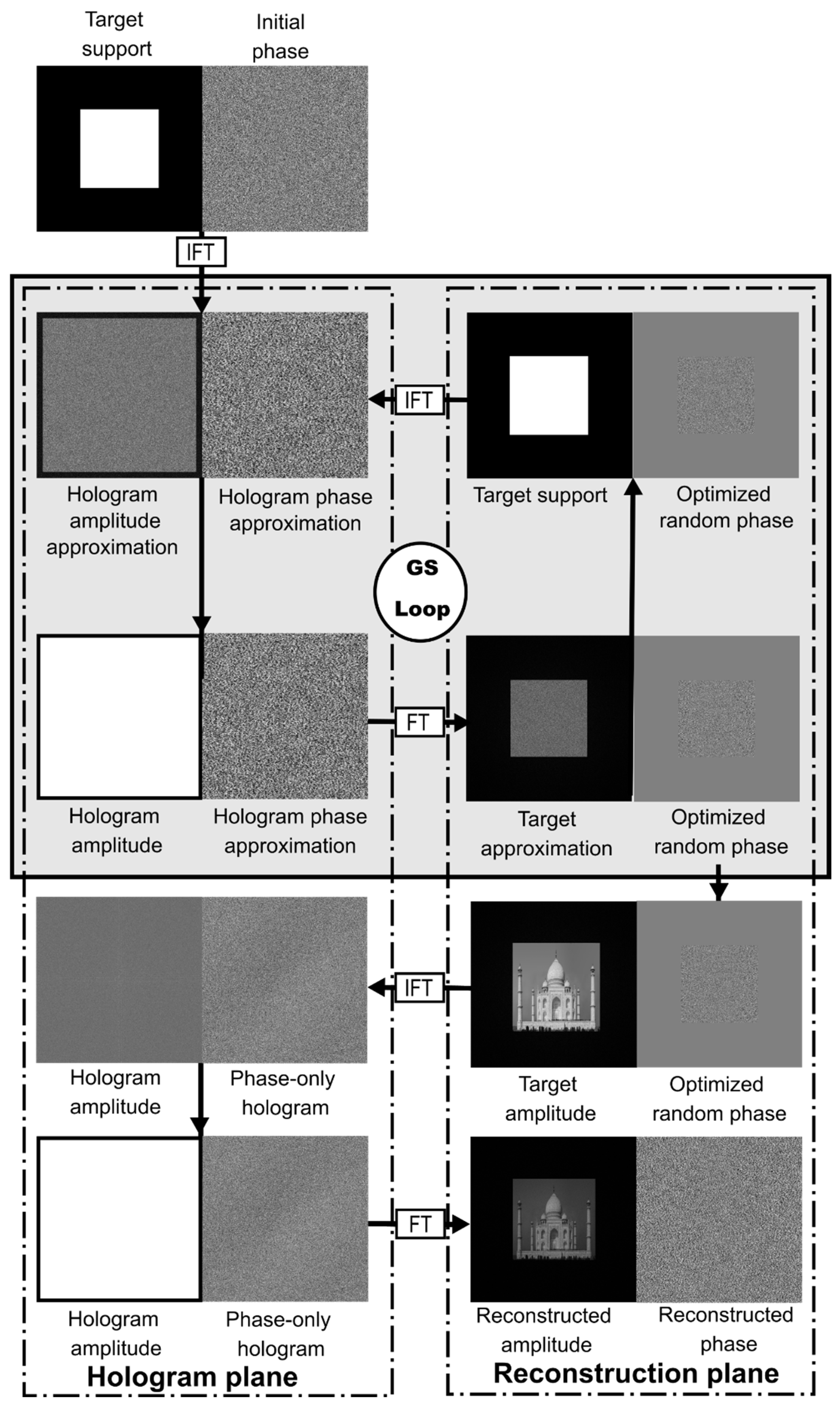
Figure 2 presents the initial random phase and the resulting optimized phases obtained using GS and SGD with the loss functions described in the previous section. It is noteworthy that the optimized phases obtained using GS and SGD for all tested loss functions exhibit a random-like structure, and the phase pattern resulting from the GS algorithm shows a clear difference outside the support area. This difference is due to the hard constraint imposed during the GS algorithm process, in which the amplitude in the reconstruction plane is replaced by the target support amplitude, as illustrated in Figure 1. In the SGD approach, this constraint is enforced indirectly by the minimization of the loss function, resulting in no visual difference between the phase inside and outside the support area.

These ORAPs were then used to generate the phase-only holograms of the same 2D target amplitude. The resulting holograms were reconstructed, and their quality was evaluated by comparing them with the original target amplitude using the CC and PSNR metrics.

The results of this test are presented in Figure 3. The phase-only hologram generated using an unoptimized random phase exhibited the lowest reconstruction quality, as indicated by the CC and PSNR metrics. In contrast, the hologram produced using the GS-based ORAP demonstrated a noticeable improvement in reconstruction quality. However, all the holograms generated using the SGD and different loss functions exhibited even higher quality, as measured by both metrics. The ORAP obtained with SGD and the $L_{mse}$ yielded the highest overall quality, followed by the $L_{psnr}$, $L_{cc}$, and, finally, the $L_{ssim}$. Although the reconstruction from the hologram generated with SGD and the $L_{ssim}$ function outperformed the GS-based ORAP, it exhibited reduced uniformity and dark regions near the image corners, particularly noticeable in the superior left corner.

To further analyze these results more effectively, a small region of interest (ROI) from each reconstruction in Figure 3 was selected to calculate the speckle contrast (SC) [35]. This analysis was relevant because the primary drawback of using random phases to generate phase-only holograms is the appearance of speckle noise in the reconstruction. The speckle contrast (SC) for an image $I$ is defined as

$$SC={\displaystyle \frac{\sqrt{〈I^2〉-{〈I〉}^2}}{〈I〉}}$$

(16)

where $〈I〉$ represents the mean value of the image. The SC takes values ranging from 0, indicating the absence of speckles or intensity fluctuations in the region of interest, to 1, which corresponds to a fully developed speckle pattern. Thus, in this test, a lower SC indicated reduced speckle degradation within region of interest of the reconstruction.

Figure 4 displays the enlarged region of interest for each reconstruction from Figure 3, along with the corresponding speckle contrast measurement for each case. Note that the unoptimized random phase reconstruction exhibited the highest level of speckle, with the speckle contrast nearly halved in the GS-ORAP case. Using SGD with all the loss functions, except for the CC loss function, resulted in an approximately 10% reduction in the SC compared with the GS-based result. As observed in Figure 2, the SGD $L_{mse}$ approach showed the best result with the lowest overall SC, with a nearly identical value to that obtained using the SGD $L_{psnr}$. It is worth noting that, although the SGD $L_{ssim}$produced the lowest CC and PSNR among all SGD-tested loss functions in Figure 3, it yielded a lower overall SC than the result obtained with the $L_{ssim}$. This suggests that $L_{ssim}$is less effective at preserving the overall contrast and structure of the original target amplitude but more effective at reducing speckle noise than the CC loss function.

We will now analyze how the reconstruction quality, as measured by the PSNR, CC, and SC for each tested method, related to the number of iterations used to obtain the ORAP.

Figure 5 presents the evolution of the reconstruction quality as a function of the number of ORAP optimization iterations using GS and SGD with different loss functions. The results indicate that SGD optimization with $L_{mse}$, $L_{psnr}$, and $L_{ssim}$ yielded faster and more significant improvements in the CC (Figure 5a), PSNR (Figure 5b), and SC (Figure 5c) as the number of iterations applied to the optimization of the ORAP increased in comparison with GS. In contrast, the SGD with the $L_{cc}$ function exhibited an initial decline in both the CC and PSNR during the first iterations, followed by a gradual recovery. After approximately 20 iterations, its performance became comparable to that of GS. Regarding the speckle contrast (Figure 5c), the $L_{cc}$ showed a trend nearly identical to that of GS, with only minor improvement observed after 20 iterations. For all the results presented in this work, 50 iterations were used for all the implemented methods to generate ORAPs. However, the results indicate that 20 iterations were sufficient to obtain an adequate ORAP with all the tested approaches, except in the case of SGD with $L_{cc}$. For SGD with loss functions other than $L_{cc}$, as well as for the GS algorithm, additional iterations yielded only marginal improvements in the reconstruction quality.

To obtain the ORAPs used for the results in Figure 3, Figure 4 and Figure 5, an RTX 3080 GPU and an Intel i9 12900K CPU were used, taking advantage of the GPU-based computation capabilities implemented via the PyTorch 2.7.0 library in the Python 3.12 programming language.

Table 1. Computation times required to obtain the ORAPs used in the results presented in Figure 3 and Figure 4.

Method	Computation Time
GS	0.246 s
SGD Lmse	0.350 s
SGD Lpsnr	0.409 s
SGD Lcc	0.463 s
SGD Lssim	1.614 s
Hologram generation with ORAP	0.002 s

presents the computation times required to generate the ORAPs using the methods discussed in Section 2.

Table 1 presents the computation time required to generate the ORAPs used in Figure 3 and Figure 4. As expected, the GS-based ORAP was the fastest to compute, requiring only 0.246 s, followed by SGD, using$L_{mse}$, $L_{psnr}$, and $L_{cc}$, with computation times ranging from 0.350 to 0.463 s. Notably, SGD with $L_{ssim}$ incurred the highest computational cost at 1.614 s due to the added complexity of evaluating structural similarity. These results highlight a well-known limitation of SGD optimization: as the complexity of the loss function increases, so does the time required to compute the gradient. It is worth noting that ORAP generation needs to be performed only once, and the resulting ORAP can be reused to generate any number of holograms of objects with the same support size. The hologram generation from an ORAP only required 0.002 s for all the results shown in this work, validating the practicality of the method. According to the results presented up to this point, the increased computation time of SGD-based ORAPs was well-justified by their capability to enable an improved reconstruction quality.

We then proceeded to evaluate the main advantage of the ORAP method: its ability to generate phase-only holograms for different scenes without the need for additional iterative procedures. For this test, we applied the ORAPs used to obtain the results in Figure 3 and Figure 4 to several distinct amplitude targets of the same size and resolution.

Figure 6 illustrates the effect of the contrast of the amplitude target on the quality of numerical reconstructions using ORAPs generated with GS and SGD optimized via different loss functions. As shown, lower-contrast amplitude targets with smoother intensity variations (center and right columns) were reconstructed with a higher quality across all ORAP variants, as measured by both the CC and PSNR. However, it is important to note that the improvements achieved with SGD using $L_{mse}$ and $L_{psnr}$, which were evident in the lower-contrast amplitude targets, were not observed in the high-contrast amplitude target shown in the left column of Figure 6 when compared with GS and SGD with $L_{ssim}$ ORAPs.

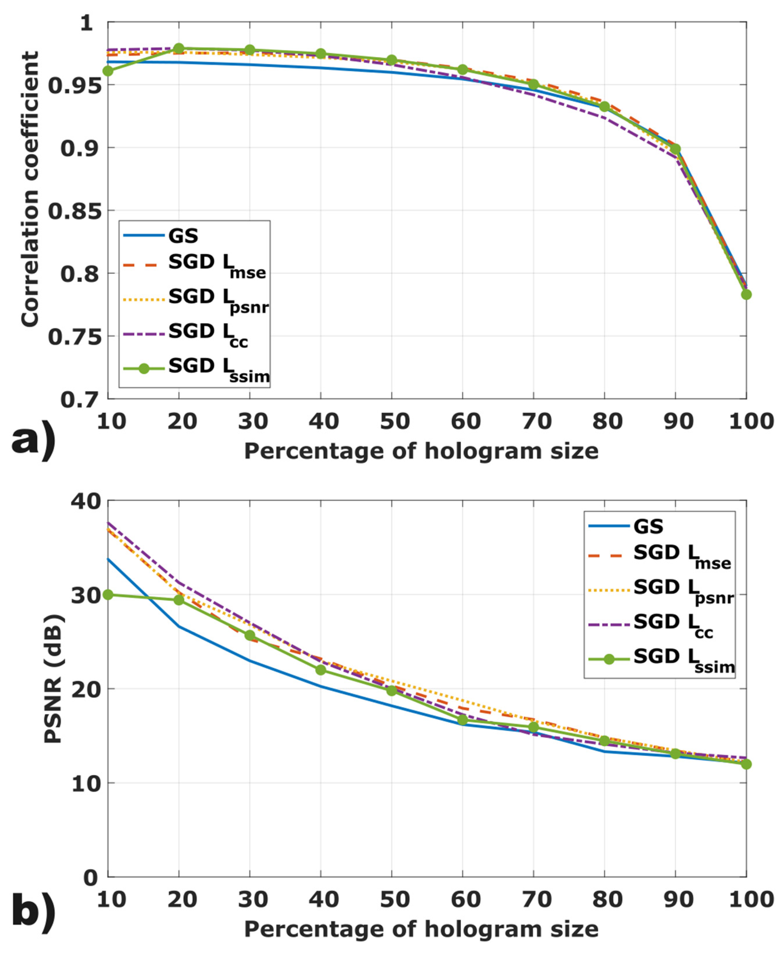
Finally, we tested how the ORAPs generated with GS and SGD performed when using different support sizes. To achieve this, we generated ORAPs for different target support sizes using GS and SGD with the four previously discussed loss functions. The target support sizes ranged from 10% and 100% of the hologram size. Once all ORAPs were obtained for each method and support size, we used them to generate the hologram of the amplitude target of Figure 3, scaled to the different support sizes used in the ORAP generation. The resulting holograms were then reconstructed, and we computed the CC and PSNR between the reconstructed amplitude and the scaled target amplitude in each case.

Figure 7 shows the results of this test. As the target support size increased from 10% to 100% of the hologram area, both the CC (Figure 7a) and the PSNR (Figure 7b) consistently decreased across all methods, indicating a degradation in the reconstruction quality with the increasing support size. Among the tested methods, the SGD-based approaches, particularly those optimized with $L_{mse}$ and $L_{psnr}$, achieved the highest reconstruction fidelity across the entire range of support sizes. All SGD implementations consistently outperformed the classical GS algorithm, especially within the 10% to 50% range, where the performance gap became more pronounced. However, the GS- and SGD-based approaches exhibited a similar performance when the support size equaled the full hologram size.

4. Experimental Results

We proceeded to experimentally reconstruct the holograms generated using the ORAPs from the previous section. To this end, we employed the holographic projection setup shown in Figure 8.

The experimental setup was based on a GAEA-2 spatial light modulator (SLM), HOLOEYE Photonics AG, Berlin, Germany, whose resolution of $3840\times 2160$ matched the resolution of the generated holograms. This device had a pixel size of 3.74 μm. Prior to being displayed on the SLM, the holograms were multiplied by a phase grating to avoid superposition between the reconstructed objects and the undiffracted light. Illumination was provided by a FISBA READYBeam Ind 2 laser, FISBA AG, St. Gallen, Switzerland, emitting at a wavelength of 520 nm, with an output power of 30 mW. The laser was coupled to a 3 μm single-mode fiber. To convert the divergent output from the fiber into a collimated beam, a collimation system comprising an adjustable iris and a 400 mm focal length converging lens was employed. A second converging lens with a 20 cm focal length was used to perform the Fourier transform of the holograms. The reconstructions were recorded using a Canon EOS R8 camera, Canon, Tokyo, Japan, with a resolution of $6000\times 4000$ and a pixel size of 6 μm.

The experimental results from projecting the holograms generated in the previous section are shown in Figure 9. It can be observed that the reconstruction quality was nearly identical across all methods, with only the result obtained using SGD with $L_{ssim}$ showing a slight difference. This was manifested as darker regions near the corners of the reconstruction and a proportionally increased brightness at the center. To better evaluate the differences between the reconstructions obtained from the holograms generated using ORAPs with all the discussed methods, we selected a region of interest in the reconstructions of the object shown in the first row of Figure 9 and computed the CC and PSNR with respect to the original object.

The results of this test are shown in Figure 10. Despite the visual similarity across all reconstructions, the results show a consistent, slight improvement over the GS approach in both the CC and PSNR for ORAPs generated using SGD with all the loss functions, except for $L_{ssim}$, which exhibited lower CC and PSNR values than GS.

The overall similarity between the reconstructions obtained using SGD- and GS-optimized ORAPs may be attributed to the significant speckle noise introduced by the experimental setup. Contributing factors included pixel crosstalk in the SLM, particularly affecting holograms with near-random phase distributions, such as those generated using ORAPs, as well as aberrations introduced by the reconstruction lens. Nevertheless, the results confirm that SGD, with all the tested loss functions, is a viable alternative to the standard GS-ORAP approach. The flexibility provided by SGD through custom loss functions suggests its potential for further improvement. In particular, incorporating loss functions that account for the physical characteristics of the optical setup and light propagation [36] may enable future implementations of SGD-ORAP to achieve superior experimental performance compared with GS-ORAP.

5. Discussion

The numerical results in Figure 3 and Figure 4 indicate that ORAPs optimized using SGD produced a superior reconstruction quality compared with GS-ORAPs, as evidenced by the higher CC and PSNR values and lower speckle contrast, particularly when the $L_{mse}$ and $L_{psnr}$ loss functions were employed. Among the tested loss functions, SGD with MSE loss yielded the highest overall performance. Notably, all SGD-optimized ORAPs performed significantly better on low-contrast targets than the GS-ORAP, as shown in Figure 5. This behavior is likely attributable to the similarity between these targets and the rectangular support function used during optimization. Importantly, while the initial generation of SGD-ORAPs incurred a modest additional computational cost, their reusability across diverse targets offered a compelling trade-off between reconstruction quality and computational efficiency. Additionally, although Table 1 shows that ORAP generation using SGD with all the tested loss functions required slightly more computation time than GS for 50 iterations, the results in Figure 5 indicate that 20 iterations or less for SGD were sufficient for all loss functions except $L_{cc}$.

Figure 7 further demonstrates that SGD-ORAP led to holograms with improved reconstructions across all target support sizes compared with GS-ORAP. However, this improvement diminished as the support sizes increased. A possible explanation of this effect is that the area outside the support is not considered during the loss function evaluation. As the support becomes smaller, optimization becomes easier because there are more pixels outside the support that can be freely adjusted to minimize the loss within the support area.

Finally, the optical reconstructions shown in Figure 9 and Figure 10 reveal minimal visual differences between the optical reconstruction of holograms generated with ORAPs using GS and SGD across all the tested loss functions. However, a slight improvement in the CC and PSNR was observed when employing SGD. As noted in the previous section, the comparable quality across the methods in experimental reconstructions may stem from noise sources in the holographic projection setup, absent in the numerical simulations, that potentially mask the quality enhancements achieved by the proposed methods. Nevertheless, these findings confirm that the SGD-ORAP method is a viable approach to the non-iterative generation of holograms.

Compared with recent advances in non-iterative hologram generation, most of which rely on convolutional neural networks (CNNs), the ORAP concept shown in this work offers a more accessible and computationally efficient alternative. Advanced CNN-based strategies, such as camera-in-the-loop setups [37], propagation error compensation [38], and learned light transport [36], can achieve a higher reconstruction quality than those reported in this work. However, CNN-based approaches require large datasets and a substantial training time. In contrast, ORAPs can be computed in under one second for most of the tested loss functions. Furthermore, CNNs typically demand significant memory to store trained parameters, which may limit their practicality in some scenarios. In ORAP-based holography, only the ORAP and the target amplitude need to be stored, often requiring less than 20 MB for high-resolution holograms such as those used in this work. The final hologram is then obtained through a simple multiplication followed by an inverse Fourier transform, enabling very fast hologram generation.

6. Conclusions

We proposed and evaluated for the first time, to the best of our knowledge, a non-iterative method for phase-only hologram generation, employing stochastic gradient descent (SGD) to optimize random phase functions. By minimizing loss functions based on common image quality metrics, specifically MSE, PSNR, CC, and SSIM, we generated optimized random phase masks (ORAPs) that can be reused across multiple target amplitudes with the same support size, enabling non-iterative hologram generation.

The numerical results show that the SGD method with all the tested loss functions presented an improved ORAP generation performance with a minimal computational cost compared with the GS algorithm. Furthermore, the experimental results show that the performance of SGD-ORAPs was nearly identical to that of GS-ORAP across all four evaluated loss functions. These findings confirm that SGD is a viable approach for non-iterative hologram generation based on ORAPs. Moreover, SGD expands the design space through customizable loss functions, making it a promising alternative to conventional GS-based phase-tailoring methods.

Future research could explore improvements in reconstruction quality through alternative loss functions tailored to the spectral properties of target amplitude distributions or the specific characteristics of experimental setups. Additionally, combining multiple image quality metrics into a unified loss function, or extending this approach to patterned or quadratic random phases, may further enhance the quality of phase-only holograms. Finally, the added flexibility of SGD over the GS algorithm implies that the random phase optimization presented in this work could also be applied to obtain optimized phase functions for the generation of Fresnel holograms representing a broader range of scenes beyond 2D objects.