Effects of Detector Configuration on X-Ray Luminescence Computed Tomography Imaging

Abstract

Background: X-ray luminescence computed tomography (XLCT) has emerged as a promising hybrid biomedical imaging modality for over a decade. However, the detector’s configuration has not been studied. Methods: We have built a benchtop XLCT imaging system and designed different detector holders to adjust the detector’s orientations and distances. Phantom experiments were performed to evaluate the performance of the detector’s configurations. We have also performed a Monte Carlo simulation to study the detectable photon numbers. Results: The photon detection efficiency is reduced by more than 10 times as the detector orientation is changed from 0 degrees to 45 degrees. The efficiency is not reduced as the detector is up to 10 mm away from the object. The efficiency is reduced by 33% when the distance is 30 mm. The numerical simulation indicates that a ring detector improves the collection efficiency by 11.3 times. Conclusions: The XLCT’s detector configuration plays a major role in the XLCT imaging system design. In the future, a ring detector will enhance the detection efficiency of XLCT imaging.

1. Introduction

One of the most common methods of medical imaging is the X-ray and since its inception has been adapted in many ways [1]. Each utilizes X-rays to reconstruct an image of a region of interest (ROI) allowing medical professionals to deliver accurate care [2,3]. One of the most popular is X-ray computed tomography (CT) which obtains the anatomical information of objects within tissues [4,5,6,7]. This method has also been improved using reconstruction algorithms and different applications of the technology [8,9]. Among these is X-ray Luminescence Computed Tomography (XLCT), which has made impressive strides in the last 15 years since Guillem Pratx et al. performed one of the first XLCT experiments [10]. XLCT utilizes nanophosphors that emit optical photons at wavelengths within the visible-to-near-infrared (vis-to-NIR) range when excited by high-energy X-ray photons. As far back as 2012 this technique was capable of spatial resolutions below 1 mm [11]. In the following studies, Zhang et al. demonstrated that it is possible to obtain the spatial resolution of XLCT imaging close to twice the size of the pencil beam diameter [12]. Then, with the improved scanning method, Zhang et al. further improved the spatial resolution of XLCT to be the diameter of the pencil beam [13]. Lun et al. performed phantom experiments to verify that XLCT can image the phosphor target at a concentration of 0.01 mg/mL in a deep turbid media [14]. These studies are crucial for extracting information about both anatomical and functional information found within the region of interest during imaging, especially in biomedical research using small animal models.

After 15 years of XLCT imaging development, two types of XLCT imaging systems based on the X-ray beam patterns have emerged. One type is the cone beam-based XLCT imaging, in which the cone beam X-ray is used to excite the imaged object [15,16,17]. The advantage of this method comes from the fast scanning speed. The disadvantage is its limited spatial resolution. Another type is the pencil beam-based XLCT imaging, in which a collimated or a focused superfine X-ray beam scans the object sequentially [18]. The pencil beam XLCT imaging can achieve a spatial resolution up to the superfine beam size (about 150 micrometers or better) [13]. The disadvantage of this method is the long scanning time.

Currently, our lab pursues pencil beam-based XLCT imaging because of its potential for high spatial resolution when imaging deep targets. To overcome its disadvantage of slow scanning speed, we proposed a multiple X-ray beam scanning method [19]. However, the improvement is limited by the number of X-ray beams. Furthermore, we have also developed a continuous scan scheme for superfast XLCT scanning [20]. The superfast scanning method makes it possible to have three-dimensional XLCT images in a reasonable time. However, its scanning speed is still limited by the collection efficiency of the single fiber bundle-based detector.

At first, an electron multiplying charge-coupled device (EMCCD) was used to collect the emitted optical photons on the object’s surface for XLCT image reconstruction [12]. The EMCCD can acquire the measurements on the whole surface so that the measured number of photons is large. However, due to the long exposure time and the low optical photon number, the measurement time is very long for each linear scan step. Then, we demonstrated that the measurement from one single fiber bundle with a photomultiplier tube (PMT) is sufficient for XLCT image reconstruction [18]. After this study, we used the single fiber bundle-based detection module for XLCT imaging due to its high measurement sensitivity.

So far, there is no systematic study on the detector’s configuration and its effects on the scanning speed and the image quality. The configuration parameters include the detector distance to the object, detector orientation, and detector number. This paper addresses these issues with both numerical simulations and phantom experiments.

The paper is organized as follows: In the Method and Materials Section, we describe the XLCT imaging system, the phantom geometry, and the numerical simulation setup. Then, in the Results Section, we describe the major results obtained. Finally, we conclude the paper with discussions.

2. Methods and Materials

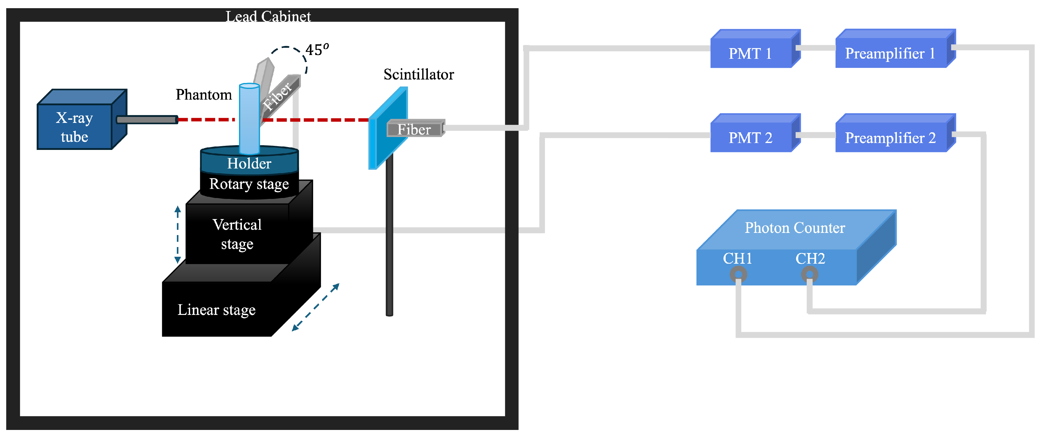
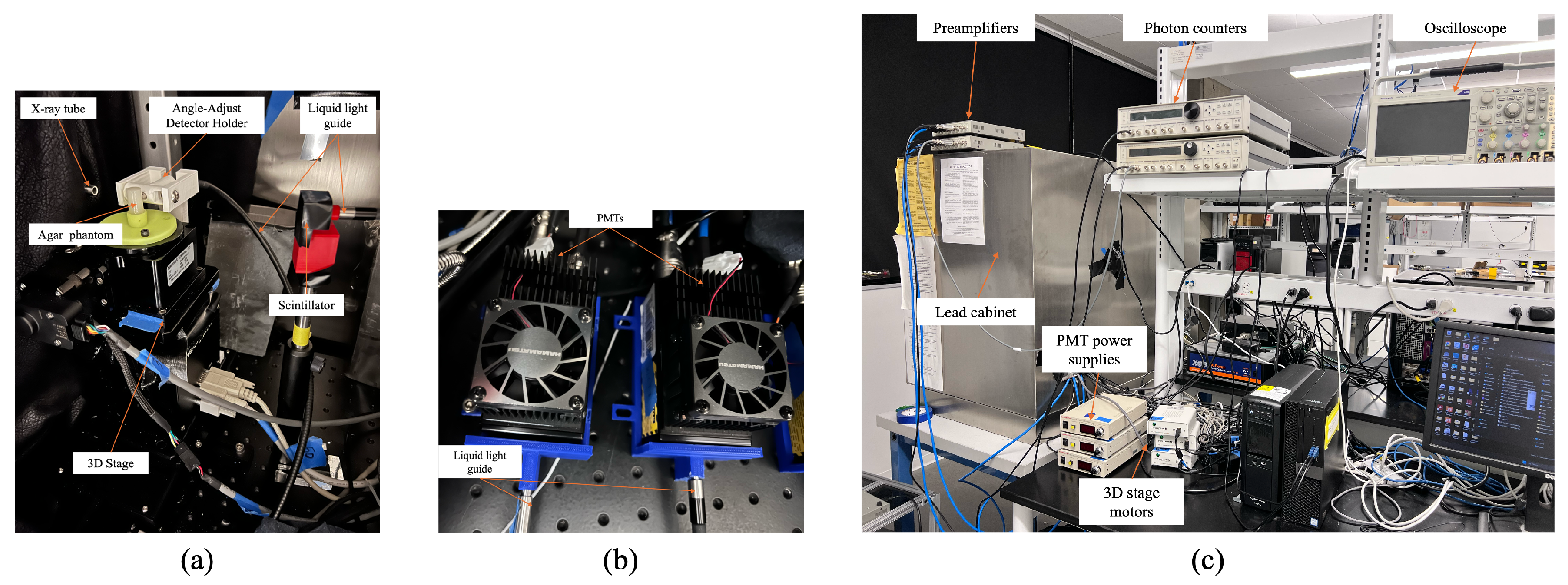
2.1. XLCT Imaging System

We described the lab-made X-ray luminescence computed tomography imaging system in our previous publications [20]. Figure 1 plots the schematic of the XLCT image. Figure 2 shows the photos of the system. Briefly, an X-ray tube with an optics lens (x-Beam Powerflux [Mo anode], XOS) forms a focused X-ray beam which scans one transverse section of the object in a manner like that of the first generation of CT scan. The object was placed on a powerful linear stage (NLE-100, Newmark Systems Inc., Rancho Santa Margarita, CA, USA), on which we mounted a motorized vertical stage (RT-3, Newmark System Inc.) and a rotary stage (VS-50, Newmark Systems Inc.). A small portion of the emitted optical photons were collected by a fiber bundle and sensed by a PMT. We have two PMTs in this system because the 2nd PMT was used to collect the photons from a scintillator-based X-ray beam detector. The electronic signals from both PMTs were amplified with pre-amplifiers (SR455A, Standford Research Systems, Sunnyvale, CA, USA), filtered with low-pass filters (BLP-10.7+, fc = 11 MHz, Mini-Circuits), and finally collected by a photon counter (SR400, Stanford Research System). The whole imaging system except for the electronics parts was placed inside an X-ray shielding and optical tight cabinet as shown in Figure 2.

To obtain the XLCT image of a transverse section, the linear stage moved the object linearly about 15 millimeters (mm) for each of the angular projections. The total angular projection number was 180 with an angular step size of 2 degrees. The total scanning time per transverse section was about 30 min, with a scanning speed of 2 mm per second continuously. And the optical photon collection time window was 10 ms. We acquired both the XLCT signals and the microCT signals simultaneously with the two PMTs. We can obtain three-dimensional (3D) XLCT images by scanning different transverse sections.

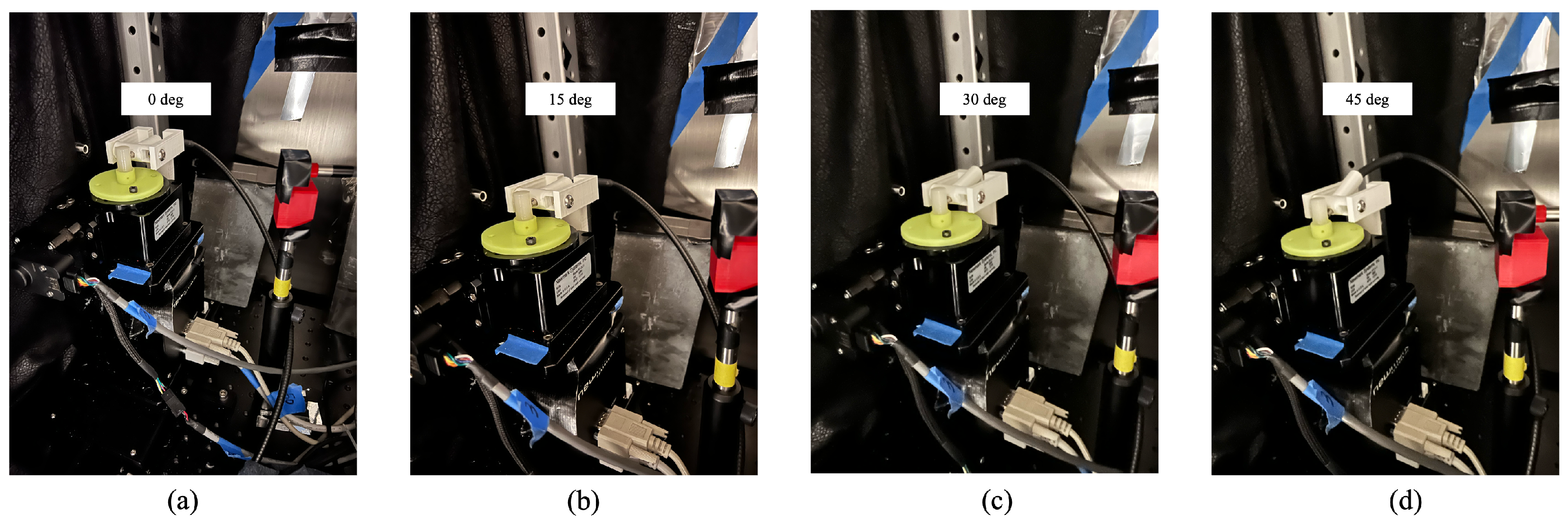
2.1.1. Detector Orientation Adjustment

In our previous studies, we always made the optical fiber bundle perpendicular (0 degrees) to the cylindrical phantom side surface. To investigate how the optical fiber bundle orientation affects the photon collection efficiency, we designed and printed a novel fiber bundle holder to adjust the orientations of the fiber bundle as shown in Figure 3, in which the white piece of plastic is the printed fiber bundle holder. We tested four different orientation angles: 0, 15, 30, and 45 degrees. We selected the range from 0 to 45 degrees since it covered the majority of the possible detector orientation angles and was sufficient to observe the trend in how the angle changes affect the measurements. Choosing the step size of 15 degrees was adequate for observing the trend and the subsequent data analysis. For each orientation, we scanned the same transverse section for each of the three unique phantoms as described in Section 2.2.

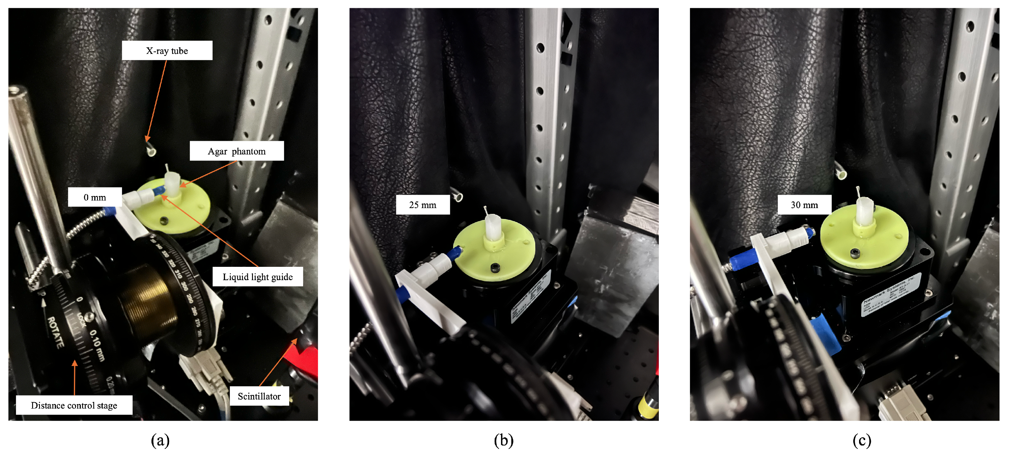
2.1.2. Detector Position Adjustment

To investigate how the distance between the fiber bundle and the side surface of the phantom (or the scanned object) affects XLCT measurements and imaging, we designed a setup to adjust the distance, as shown in Figure 4, in which the fiber bundle was fixed on a compact translational platform, a mechanical jack (LJ 750, Thorlabs, Newton, NJ, USA) with a maximum extension distance of 25.4 mm. After each measurement, we manually adjusted the jack for different distances from 0 mm to 30 mm. To achieve a distance of 30 mm which is beyond the jack extension distance, we manually moved the fiber bundle 4.6 mm away and calibrated the distance with a meter. For each distance, we performed a linear scan to analyze the measurement data. We performed two sets of measurements: One set had three different orientation angles of 0, 1, and 2 degrees with a step size of 1 degree. Another set of measurements also had three different orientation angles 0, 10, and 20 degrees with a step size of 10 degrees.

We also performed XLCT imaging for the phantom with four central targets (as described in Section 2.2) with distances of 1.5 mm and 4.5 mm.

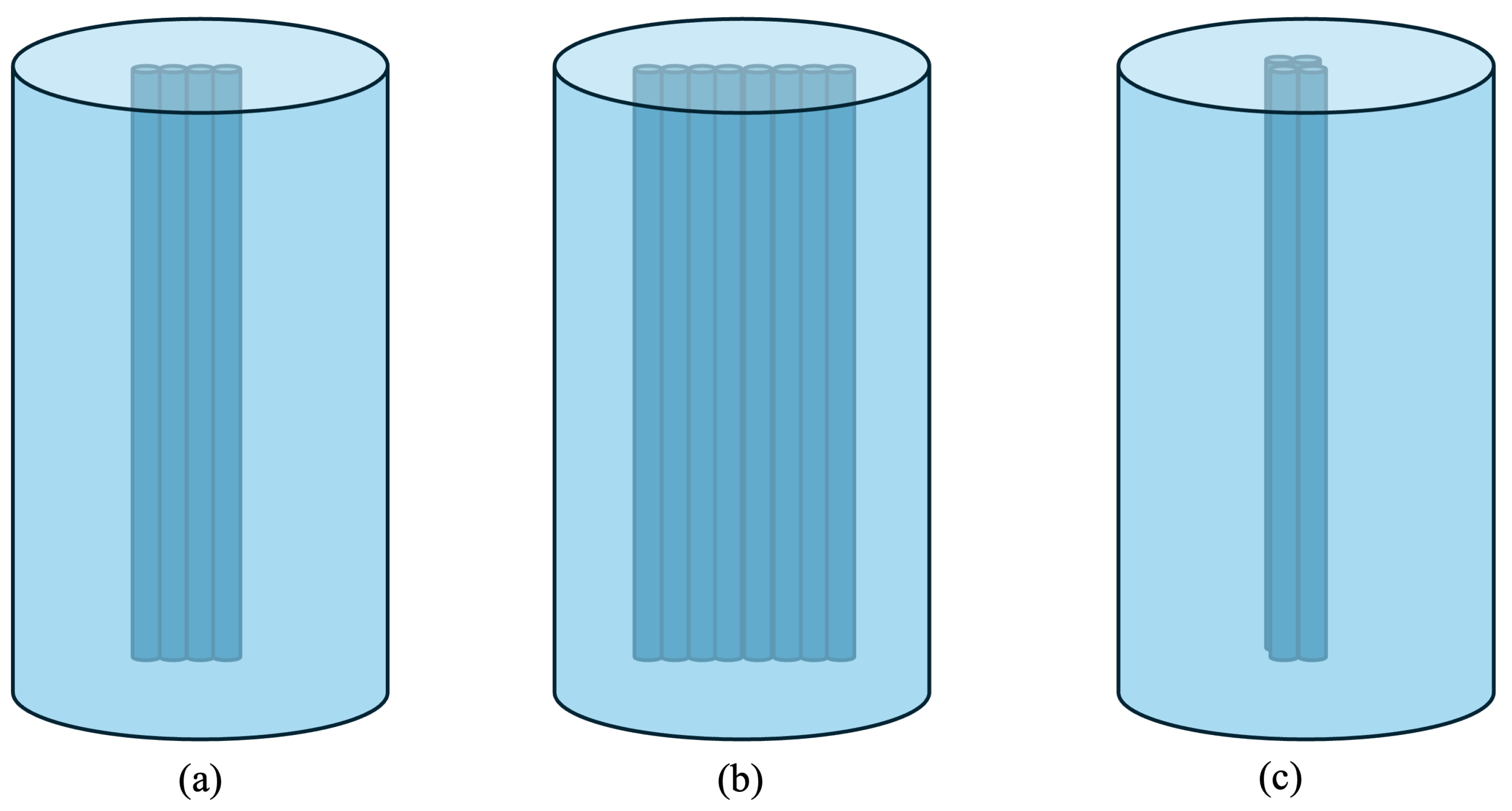
2.2. Phantom Design and Fabrication

We designed and fabricated phantoms with 3 different targets, as shown in Figure 5. The background phantom is cylindrical with a diameter of 12 mm and a height of 30 mm. The phantom was fabricated with 1% intralipid, 2% agar, and 97% water. The targets were transparent capillary tubes with an inner diameter of 0.4 mm and an outside diameter of 0.8 mm. These capillary tubes were filled with Gadolinium Oxysulfide doped with Europium ($G{d}_2{O}_{2}S$:Eu³⁺) particle solution at a concentration of 10 mg/mL. We have also added 2% agar inside the target solution to solidify the solution. We embedded the capillary tubes inside the cylindrical agar phantom for three cases: (a) four central targets in a row; (b) eight central targets in a row; and (c) four central targets that are adjacent to each other.

The XLCT imaging probe we used in this study is $G{d}_2{O}_{2}S$:Eu³⁺, which is a well-established phosphor material that exhibits strong luminescence under X-ray excitation, making it a promising candidate for XLCT imaging applications. One of its emission peaks is at 700 nm which offers relatively low absorption and scattering in biological tissues [21]. This makes the phosphor suitable for optical signal collection in small animal imaging. Therefore, using this material in our detector configuration study provides a relevant and practical basis for evaluating the performance of the system. Its well-characterized luminescence behavior under X-ray excitation ensures consistent signal generation, allowing us to focus on the impact of detector arrangements without introducing uncertainties from probe variability.

2.3. XLCT Reconstruction Algorithms

Here, we used the filtered back projection (FBP) as the reconstruction algorithm for both the XLCT images and the pencil-beam-based microCT images. FBP with the Ramp filter was selected because it is straightforward to apply. In our study, the reconstruction code was implemented in MATLAB. Briefly, the equation of the FBP can be written as follows:

$$f(x,y)={\int }_0^{2\pi }{g}_{\theta }(xcos\theta +ysin\theta )d\theta$$

(1)

where $g_{\theta }=h\left(r\right)\ast p_{\theta }\left(r\right)$ is the filtered projection and $p_{\theta }\left(r\right)$ is the measurement at projection $\theta$ and h(r) is the filter.

2.4. Criteria of Image Quality

For this study, two criteria were used to assess the quality of the reconstructed XLCT images: dice similarity coefficient (DICE) and contrast noise ratio (CNR). The DICE was calculated as follows:

$$DICE={\displaystyle \frac{2\times [RO{I}_r\cap RO{I}_t]}{|RO{I}_r+RO{I}_t]}}\times 100\%$$

(2)

where $RO{I}_r$ is the region of interest (ROI) from the reconstructed image. $RO{I}_t$ is the ROI from the ground truth image. In this study, $RO{I}_t$ is extracted from the reconstructed pencil beam micro-CT image, which serves as the ground truth image. Typically, a DICE score close to the DICE 100% indicates better image quality.

The Contrast-to-Noise Ratio (CNR) measures the ability to distinguish between different tissues by comparing the contrast difference to the noise in the image. Higher CNR indicates better image clarity and higher diagnostic accuracy.

$$CNR={\displaystyle \frac{S_{\mathrm{roi}}-S_{\mathrm{rob}}}{\sigma }}$$

(3)

where $S_{\mathrm{roi}}$ is the mean ROI value (such as target), $S_{\mathrm{rob}}$ is the mean background value, and $\sigma$ is the standard deviation of background noise.

2.5. XLCT Measurement Analysis

To analyze the effects of the detector distance on the photon collection efficiency, we used a phantom with one capillary tube target to perform a linear scan for two sets of three different angular projections (0, 1, and 2 degrees; 0, 10, and 20 degrees). For each linear scan, we obtained two outputs: the maximum photon counts among these linear scan steps and the sum of all photon counts for all linear steps of each linear scan. The maximum photon count came from the linear step when the X-ray beam passed through the target that emitted visible photons.

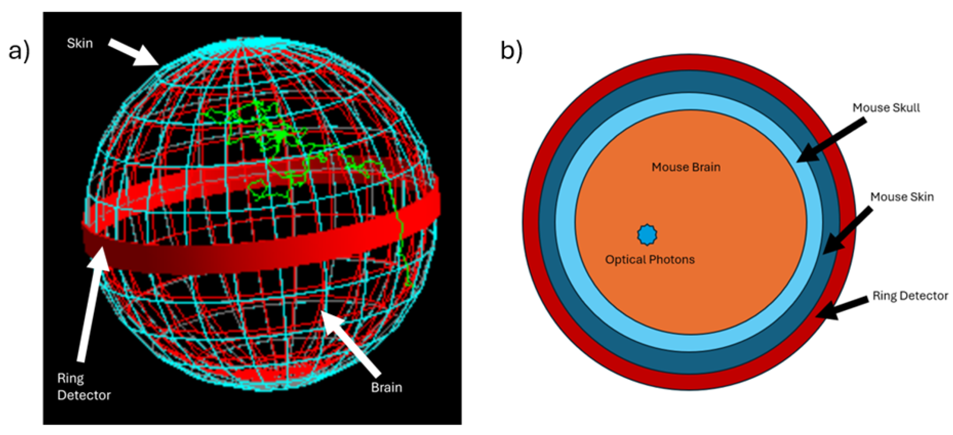
2.6. Monte Carlo Simulation Setup

To investigate the distribution of photons passing through the phantom and reaching its surface a numerical simulation was performed using Geant4 Application for Emission Tomography (GATE), a Monte Carlo simulation software (version 8.2) was installed in a 20 core CPU at 2.0 GHz and 128 GB memory, as described in [22,23]. Within the simulation environment, a spherical phantom was composed of brain tissue, skull, and mouse skin [24]. It was assigned a radius of 6 mm. Within the phantom an optical photon source generated 10⁶ optical photons at the energy of 1.99 eV. This optical photon source simulated the X-ray excitable particles emitting optical photons inside an object. Figure 6a plots the GATE simulation setup, in which the sphere simulated the geometry of an imaged object such as a mouse brain. The green curve represents a typical scattering path of an optical photon before it reaches the object’s surface. The optical source was offset by 4 mm in the transverse section of the ring detector as shown in Figure 6b. We have created a ring-ideal photon detector with 0.1 mm thickness and 1 mm in height. The ideal detector detected and absorbed all the detected optical photons. The Cartesian coordinates of each photon that made contact with the detector were recorded.

3. Results

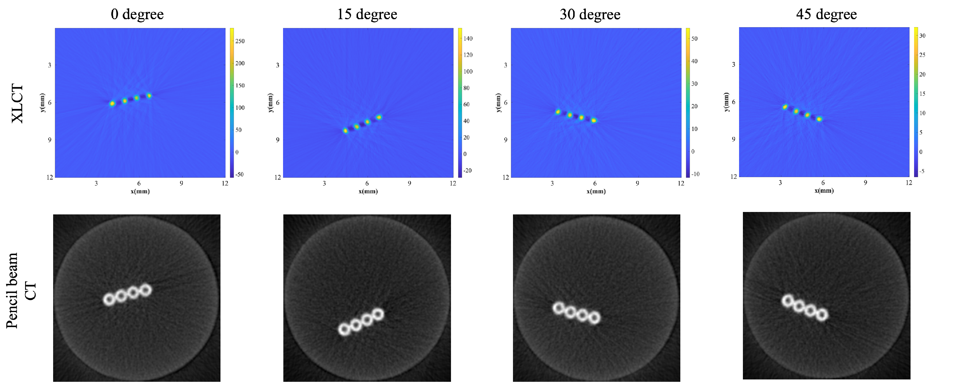
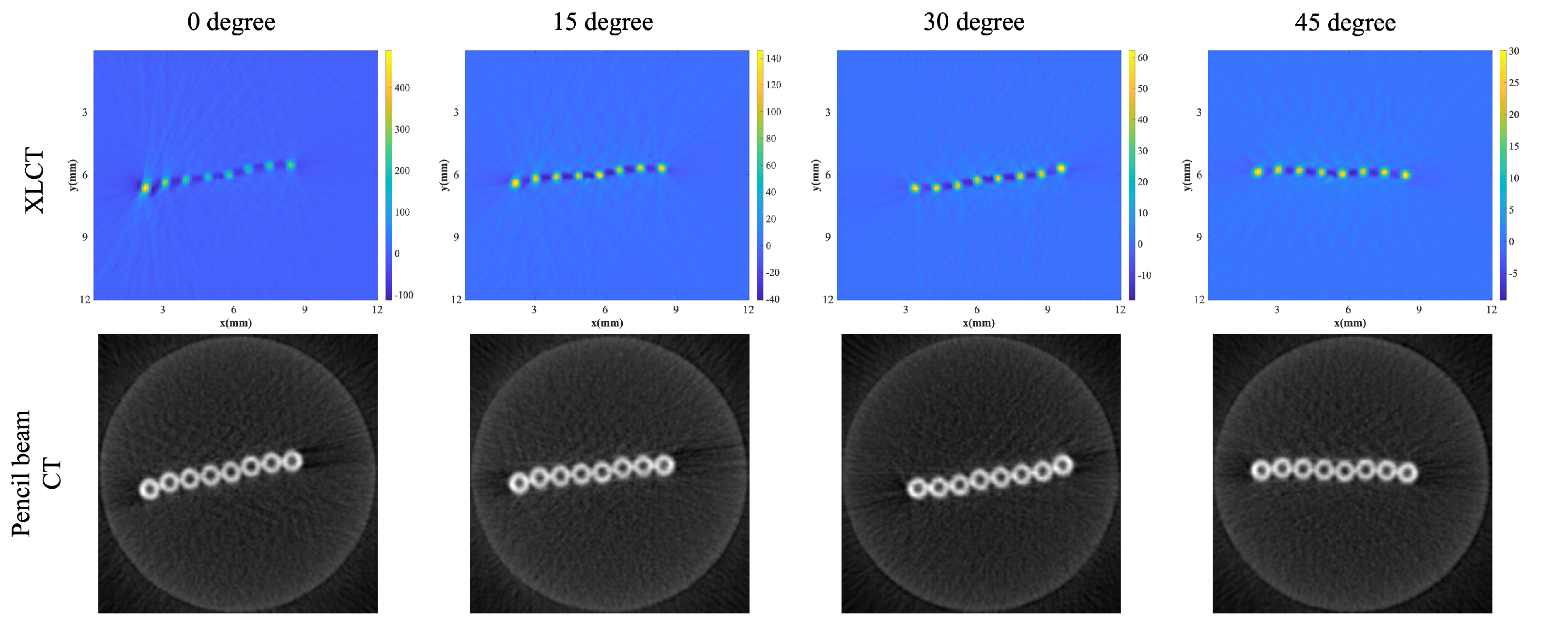
3.1. XLCT Imaging with Different Orientations of the Optical Fiber Bundle

Figure 7 plots the reconstructed XLCT images (top row) and their corresponding pencil beam-based microCT images (bottom row) for the phantom with four targets in a row. We scanned the phantom with the fiber bundle’s orientation of 0 degrees (the leftmost column) and repeated the scans for the orientations of 15 degrees (the second column from left), 30 degrees (the third column from left), and 45 degrees (the rightmost column). All the XLCT images have been reconstructed very well with a DICE larger than 83.17% and a CNR larger than 14.11 as shown in

Table 1. DICEs and CNRs values for phantom reconstructions with four and eight targets at detector orientation angles of 0, 15, 30, and 45 degrees.

Phantom	Degree	DICE	CNR
4 Targets	0 deg	86.9%	14.9
	15 deg	83.77%	14.29
	30 deg	85.99%	14.11
	45 deg	83.17%	14.15
8 Targets	0 deg	76.21%	8.34
	15 deg	82.5%	9.45
	30 deg	85.99%	9.84
	45 deg	83.91%	9.38

. Although the four targets are at different locations for different scans, their true location is validated by the simultaneously scanned microCT images. As expected, we have also observed that the reconstructed signals in XLCT images decreased from 250 to 140, 50, and 30 when we changed the orientations from 0 degrees to 15, 30, and 45 degrees, respectively. Because the X-ray excitable particles (GOS: Eu3 +) had a very high concentration of 10 mg/mL in all four targets, the XLCT measurements were still large enough for a good XLCT reconstruction so that the decrease has limited impacts on the quality of the reconstructed XLCT images. It is worth noting that the orientation of the detector’s fiber bundle has resulted in a lower photon collection efficiency by about eight times when the orientation is changed from 0 degrees to 45 degrees, which must be considered during the future XLCT imaging system design.

We repeated the above experiments with another phantom of eight targets in a row and the results are plotted in Figure 8, in which all graphs are plotted in the same pattern as in Figure 7. Similarly, all XLCT images were reconstructed very well with very high DICE coefficients and CNR as shown in Table 1. Although the XLCT image quality does not deteriorate, the photon collection efficiency is reduced by more than 10 times by adjusting the orientation angle from 0 degrees to 45 degrees, as indicated by the reconstructed XLCT images in Figure 8.

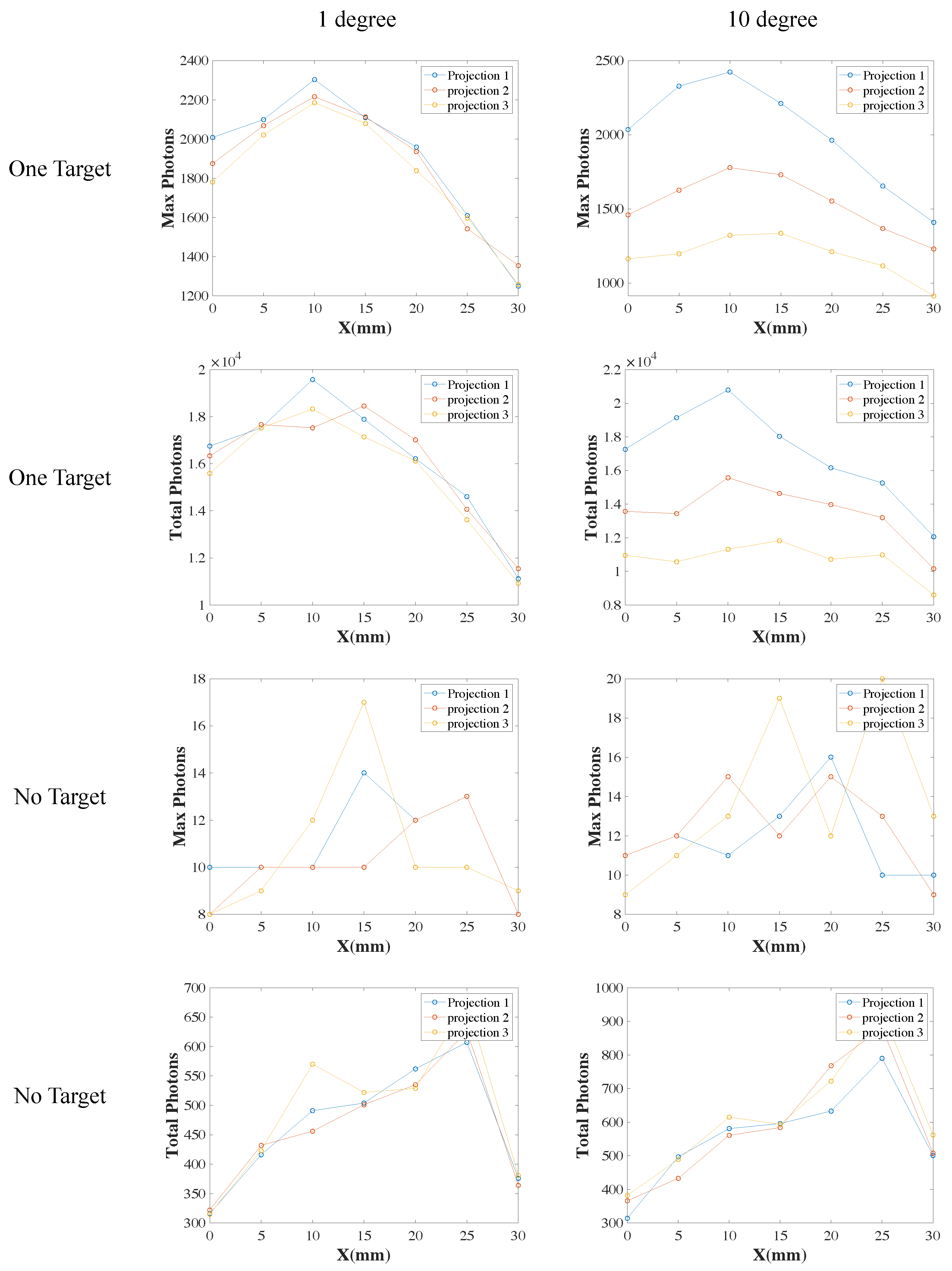
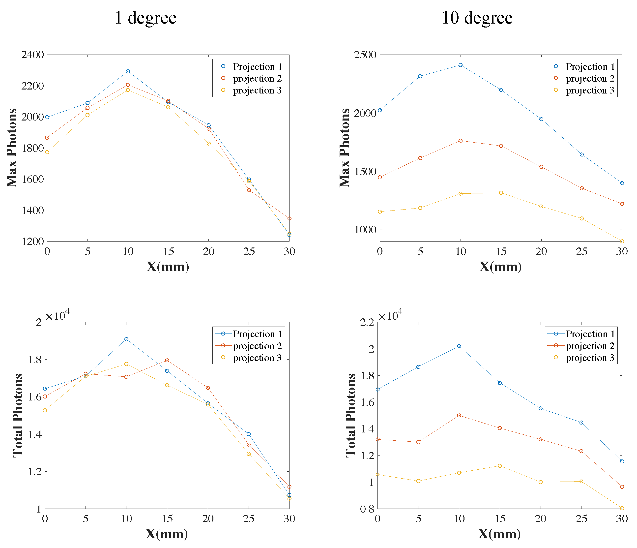
3.2. XLCT Measurements at Different Detector Distances

We have fabricated a cylindrical phantom with only one capillary tube target filled with Gd₂O₂S:Eu³⁺ particles at a concentration of 10 mg/mL. We recorded the XLCT measurements at each linear scan step for different fiber bundle distances. In Figure 9, we plotted the maximum (top row) and the total measurement (second row) for each linear scan. We repeated the experiments without targets and plotted the results in the bottom two rows of Figure 9. Then, we tilted the fiber bundle with an orientation angle of either 1 or 10 degrees and repeated the experiments and plotted the results in Figure 9. The three curves in each subfigure of Figure 9 are for the measurements of three angular projection angles (0, 1, and 2 degrees in the left column; 0, 10, and 20 degrees in the right column). To get rid of the effects of background photons on the results, we have subtracted the measurements (figures in the top two rows of Figure 9) with one target by the measurement without target (figures in the bottom two rows of Figure 9) and plot the subtracted measurements for each case in Figure 10.

We are surprised to observe that the measured photon number increased slightly up to 10% when increasing the fiber bundle distances from 0 to 10 mm. We repeated this many times, and used a black tube mounted at the end of the fiber bundle to eliminate ambient light. However, the same trend was observed. Furthermore, the same trend was observed in the subtracted measurements as shown in Figure 10, in which the effects of the electronic noises and the background lights were eliminated. When the distance increased beyond 10 mm, the measured photon number decreased almost linearly. For the distance of 30 mm, the measured photon number was reduced by 33% compared to the measurement at 0 mm.

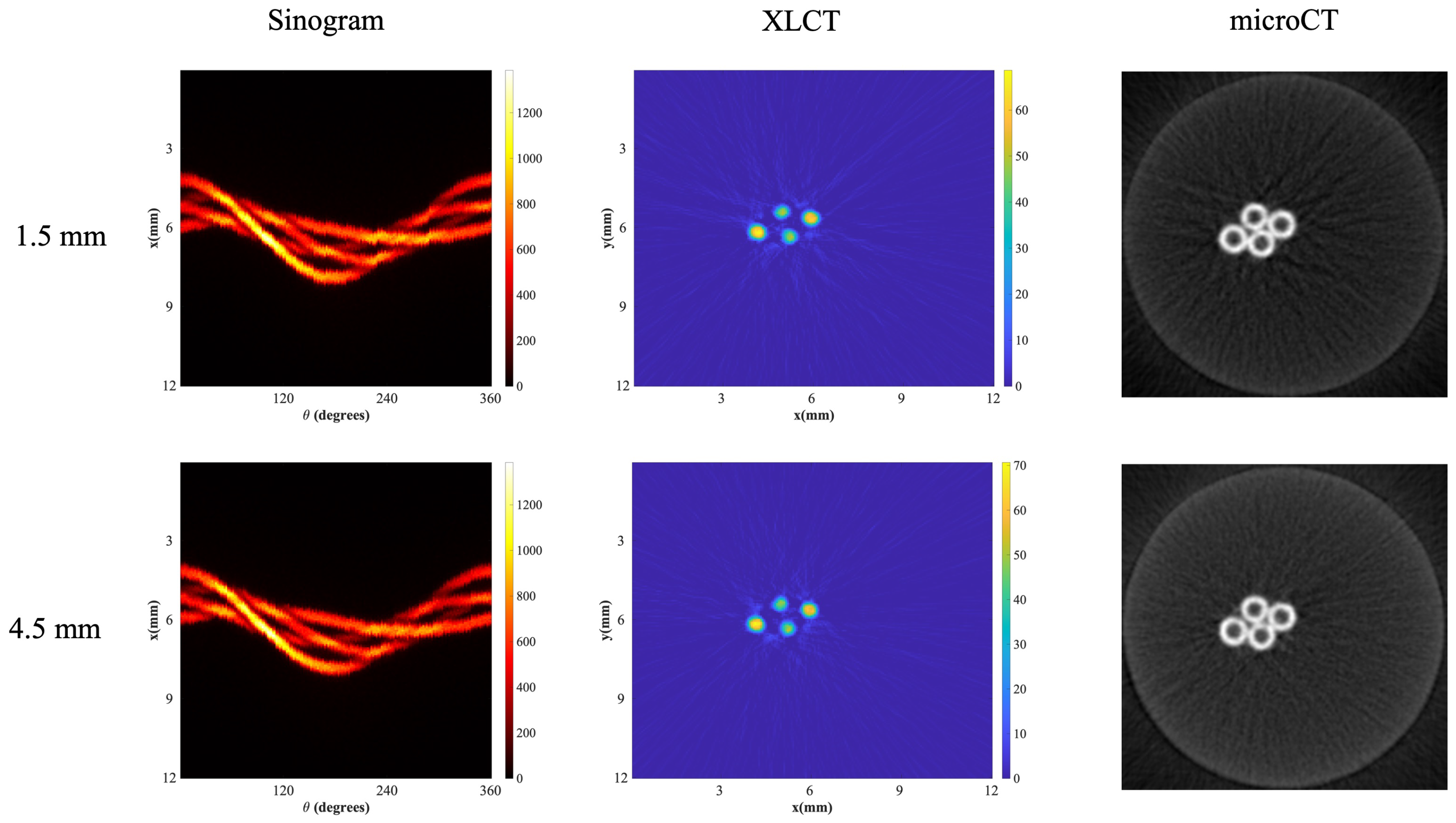
3.3. XLCT Imaging at Different Detector Distances

To verify what we observed in the top subsection, we have performed XLCT imaging for the phantom with four central targets for two different fiber bundle distances of 1.5 mm and 4.5 mm. In Figure 11, we plotted the sinograms (left column), the reconstructed images (middle column), and the corresponding pencil beam microCT images (right column). The figures in the top row and the bottom row are for the distance of 1.5 mm and 4.5 mm, respectively. The true target size and position were obtained from the simultaneous microCT images, from which we have calculated the maximum and the sum of the pixel intensities in the target region (ROI) as shown in

Table 2. Distances of 1.5 mm and 4.5 mm were studied for the four targets reconstructed images.

Distance	Max (ROI)	Sum (ROI)	DICE	CNR
1.5 mm	66.94	10715.82	71.92%	8.73
4.5 mm	68.68	10451.23	79.28%	8.2

. The maximum intensity increased slightly about 2.6% and the sum intensity reduced slightly about 2.5%, which indicates that the reconstructed intensity did not change significantly as the fiber bundle distance changed from 1.5 mm to 4.5 mm. We also calculated the DICEs and the CNRs for both cases as listed in Table 2. Both DICES are larger than 71.9% and both CNRs are higher than 8.2, which indicates that the reconstructed XLCT images have very good quality at both fiber bundle distances.

3.4. Monte Carlo Simulation Results

Of the 10⁶ optical photons in the simulation with the ring detector, 17,161 optical photons or 1.7% of the total emitted optical photons reached the ring detector. If we placed a fiber bundle with an inner diameter of 1 mm by 1 mm on the skin closest to the emission source, the detectable optical photon number is 1503, which is about 0.15% of the emitted photons. We also recorded 23.4% of the total emitted optical photons reaching the outside surface of the sphere or the skin layer of the simulated mouse brain. Our results indicate that we only detect a very small portion of the emitted photons less than 0.15% if we only use one fiber bundle-based detector for the XLCT imaging.

4. Discussion

One of the strengths of the pencil-beam-based XLCT imaging is its ability to simultaneously acquire the XLCT images and the microCT images so that the scan time and the radiation dose are reduced. Furthermore, because the two images are acquired simultaneously, the microCT image can serve as the ground truth image for XLCT reconstruction. Since we use a pencil-beam X-ray source to excite the nanoparticle, the image resolution is about the X-ray beam size, which is approximately 150 µm in this study. The imaging depth is about centimeters since both X-ray and NIR photons can penetrate into deep tissues for a whole-body mouse imaging.

While our superfine beam-based XLCT imaging system provides high-resolution imaging, the scanning time is relatively longer compared to cone-beam XLCT. In our setup, one transverse section scan takes about 30 min with 180 angular projections at a scan speed of 2 mm/s, with each linear scan covering 15 mm.

For the orientation study, at first, it is true that the detector at 0 degrees collected the most emission photons, which is very important for the XLCT imaging studies with a target with very low concentrations such as 0.01 mg/mL. Secondly, we observed that the XLCT image quality is slightly worse for the 0 degree case compared with other cases as shown in Table 1 for the eight targets phantom study. The main reason is the reconstruction algorithm (FBP without correction) we used in this study. The utilization of FBP makes the XLCT reconstruction quicker and easier to be implemented with acceptable image quality, as shown in Figure 7 and Figure 8, in which all the targets have been reconstructed very well. However, there are some artifacts due to the FBP reconstruction, especially for the target close to the boundary (the leftmost target in Figure 8). For the 0 degree case, the photons from the boundary target were scattered less compared to photons from other targets. If there is an angle more than 15 degrees, the difference of scattering effects will be reduced.

The orientation of the fiber bundle or the detector has a substantial impact on the photon collection efficiency. For the XLCT targets with high concentrations, the reduction in photon collection efficiency does not have an impact on the reconstructed XLCT image quality. For the low-concentration target and the future in vivo study in which the nanoparticle delivery is challenging, we must make sure the fiber bundle is vertical to the measurement surface for maximum photon collection efficiency.

The distance has also affected the photon collection efficiency, especially when the distance increased beyond 10 mm. We are not certain why the measured photon number increases when the distance increases from 0 mm to 10 mm, although the increase is relatively small. One possible reason is that the pre-amplifier gain may be changed during the measurements. We will investigate this topic with better electronic devices in the future. What we can learn from this study is that it is fine to keep the detector a few millimeters away from the object’s surface without reducing the measured photon numbers. It means that we can design a ring detector without touching the imaged object such as a mouse.

We also repeated the measurements of the photon number at different distances after we placed a black tube between the fiber bundle and the phantom surface to remove all the ambient light effects from the background inside the cabinet. We observed similar curves as those plotted in Figure 9. These measurements excluded the factor of the ambient photons in the measurements.

The simulation results help us understand how to design a multiple detector-based XLCT imaging system in the future. With a ring of detectors, the total photon collection efficiency increased from 0.15% to 1.7%. Further simulations can be done to determine how other detector patterns such as patch detector or spherical detector configurations affect the photon collection efficiency. Finally, we may simulate the detector orientation’s effects on the photon collection efficiency too. We may consider this approach in the future to produce the best sensitivity and short scan time for XLCT imaging, especially for the pencil beam-based XLCT imaging.

5. Conclusions

We investigated the effects of the orientation and the distance of the detector fiber bundle on XLCT imaging systematically. Our results indicate that the fiber bundle can be 10 mm away from the object’s surface without sacrificing the XLCT image quality. We also found that it is better to make the fiber bundle vertical to the object’s surface. Our simulation results indicate that the detector photon collection efficiency can be improved by 11.3 times if we utilize a ring detector compared with a single fiber bundle detector.

References

1. Ou, X.; Chen, X.; Xu, X.; Xie, L.; Chen, X.; Hong, Z.; Bai, H.; Liu, X.; Chen, Q.; Li, L.; et al. Recent development in x-ray imaging technology: Future and challenges. Research 2021, 2021, 9892152. [Google Scholar] [CrossRef] [PubMed]
2. Dong, J.; Ling, R.; Huang, Z.; Xu, Y.; Wang, H.; Chen, Z.; Huang, M.; Stankovic, V.; Zhang, J.; Hu, Z. Feasibility exploration of myocardial blood flow synthesis from a simulated static myocardial computed tomography perfusion via a deep neural network. J. X-Ray Sci. Technol. 2025, 33, 578–590. [Google Scholar] [CrossRef]
3. Yu, J.; Ding, Y.; Wang, L.; Hu, S.; Dong, N.; Sheng, J.; Ren, Y.; Wang, Z. Radiomics and deep learning features of pericoronary adipose tissue on non-contrast computerized tomography for predicting non-calcified plaques. J. X-Ray Sci. Technol. 2025, 33, 96–108. [Google Scholar] [CrossRef]
4. Wang, G.; Yu, H.; De Man, B. An outlook on x-ray CT research and development. Med. Phys. 2008, 35, 1051–1064. [Google Scholar] [CrossRef]
5. Shen, Y.; Liang, N.; Zhong, X.; Ren, J.; Zheng, Z.; Li, L.; Yan, B. CT image super-resolution under the guidance of deep gradient information. J. X-Ray Sci. Technol. 2025, 33, 58–71. [Google Scholar] [CrossRef] [PubMed]
6. Maire, E.; Withers, P.J. Quantitative X-ray tomography. Int. Mater. Rev. 2014, 59, 1–43. [Google Scholar] [CrossRef]
7. Lusic, H.; Grinstaff, M.W. X-ray-computed tomography contrast agents. Chem. Rev. 2013, 113, 1641–1666. [Google Scholar] [CrossRef] [PubMed]
8. Thilagavathi, P.; Geetha, R.; Jothi Shri, S.; Somasundaram, K. An effective COVID-19 classification in X-ray images using a new deep learning framework. J. X-Ray Sci. Technol. 2025, 33, 297–316. [Google Scholar] [CrossRef]
9. Long, Y.; Zhong, Q.; Lu, J.; Xiong, C. A novel detail-enhanced wavelet domain feature compensation network for sparse-view X-ray computed laminography. J. X-Ray Sci. Technol. 2025, 33, 488–498. [Google Scholar] [CrossRef]
10. Pratx, G.; Carpenter, C.M.; Sun, C.; Xing, L. X-ray luminescence computed tomography via selective excitation: A feasibility study. IEEE Trans. Med. Imaging 2010, 29, 1992–1999. [Google Scholar] [CrossRef]
11. Badea, C.; Stanton, I.; Johnston, S.; Johnson, G.; Therien, M. Investigations on X-ray luminescence CT for small animal imaging. In Proceedings of the SPIE, San Diego, CA, USA, 2 March 2012; Volume 8313, p. 83130T. [Google Scholar]
12. Zhang, W.; Lun, M.C.; Nguyen, A.A.T.; Li, C. X-ray luminescence computed tomography using a focused x-ray beam. J. Biomed. Opt. 2017, 22, 116004. [Google Scholar] [CrossRef]
13. Zhang, Y.; Lun, M.C.; Li, C.; Zhou, Z. Method for improving the spatial resolution of narrow x-ray beam-based x-ray luminescence computed tomography imaging. J. Biomed. Opt. 2019, 24, 086002. [Google Scholar] [CrossRef] [PubMed]
14. Lun, M.C.; Zhang, W.; Li, C. Sensitivity study of x-ray luminescence computed tomography. Appl. Opt. 2017, 56, 3010–3019. [Google Scholar] [CrossRef]
15. Liu, T.; Rong, J.; Gao, P.; Zhang, W.; Liu, W.; Zhang, Y.; Lu, H. Cone-beam x-ray luminescence computed tomography based on x-ray absorption dosage. J. Biomed. Opt. 2018, 23, 026006. [Google Scholar] [CrossRef] [PubMed]
16. Zhang, G.; Liu, F.; Liu, J.; Luo, J.; Xie, Y.; Bai, J.; Xing, L. Cone beam x-ray luminescence computed tomography based on Bayesian method. IEEE Trans. Med. Imaging 2016, 36, 225–235. [Google Scholar] [CrossRef]
17. Chen, D.; Zhu, S.; Yi, H.; Zhang, X.; Chen, D.; Liang, J.; Tian, J. Cone beam x-ray luminescence computed tomography: A feasibility study. Med. Phys. 2013, 40, 031111. [Google Scholar] [CrossRef] [PubMed]
18. Zhang, W.; Zhu, D.; Lun, M.; Li, C. Collimated superfine x-ray beam based x-ray luminescence computed tomography. J. X-Ray Sci. Technol. 2017, 25, 945–957. [Google Scholar] [CrossRef]
19. Zhang, W.; Zhu, D.; Lun, M.; Li, C. Multiple pinhole collimator based x-ray luminescence computed tomography. Biomed. Opt. Express 2016, 7, 2506–2523. [Google Scholar] [CrossRef]
20. Fang, Y.; Zhang, Y.; Lun, M.C.; Li, C. Superfast scan of focused X-ray luminescence computed tomography imaging. IEEE Access 2023, 11, 134183–134190. [Google Scholar] [CrossRef]
21. Michail, C.; Valais, I.; Seferis, I.; Kalyvas, N.; David, S.; Fountos, G.; Kandarakis, I. Measurement of the luminescence properties of Gd2O2S: Pr, Ce, F powder scintillators under X-ray radiation. Radiat. Meas. 2014, 70, 59–64. [Google Scholar] [CrossRef]
22. Cortez, J.; Romero, I.; Ngo, J.; Azam, M.S.T.; Niu, C.; Almeida-da Silva, C.L.C.; Cabido, L.F.; Ojcius, D.M.; Chin, W.C.; Wang, G.; et al. Multiple energy X-ray imaging of metal oxide particles inside gingival tissues. J. X-Ray Sci. Technol. 2024, 32, 87–103. [Google Scholar] [CrossRef] [PubMed]
23. Romero, I.O.; Fang, Y.; Li, C. Correlation between X-ray tube current exposure time and X-ray photon number in GATE. J. X-Ray Sci. Technol. 2022, 30, 667–675. [Google Scholar] [CrossRef] [PubMed]
24. Soleimanzad, H.; Gurden, H.; Pain, F. Optical properties of mice skull bone in the 455- to 705-nm range. J. Biomed. Opt. 2017, 22, 010503. [Google Scholar]
Figure 1. The schematic of the XLCT imaging system.
Photonics 12 00483 g001
Figure 2. Photograph of the XLCT imaging system. (a) The X-ray tube, the stages, and the fiber bundle inside a cabinet. (b) The two PMTs. (c) The electronic components outside the cabinet.
Photonics 12 00483 g002
Figure 3. The optical fiber bundle at different orientations: (a) 0 degrees; (b) 15 degrees; (c) 30 degrees; and (d) 45 degrees.
Photonics 12 00483 g003
Figure 4. The optical fiber bundle at different distances from the imaged phantom: (a) 0 mm; (b) 25 mm; and (c) 30 mm.
Photonics 12 00483 g004
Figure 5. Cylindrical phantom with different targets: (a) 4 targets in a row; (b) 8 targets in a row; and (c) four central targets.
Photonics 12 00483 g005
Figure 6. (a) GATE Simulation setup. (b) A transverse slice of the simulation setup. The source of the optical photons is offset by 4 mm in the transverse section. This is within the brain tissue sphere. The second layer is the mouse skull, and the third layer is the mouse skin while the final layer is the plexiglass detector.
Photonics 12 00483 g006
Figure 7. Four different orientations of the fiber bundle, the reconstructed XLCT image (top row) and microCT images (bottom row) for the phantom with four targets in a row. Left most column for 0 degrees; the second column from the left for 15 degrees; the third column from the left for 30 degrees; and the right most column for 45 degrees.
Photonics 12 00483 g007
Figure 8. Eight different orientations of the fiber bundle, the reconstructed XLCT image (top row) and microCT images (bottom row) for the phantom withe eight targets in a row. Left most column for 0 degree; the second column from the left for 15 degrees; the third column from the left for 30 degrees; and the right most column for the 45 degrees.
Photonics 12 00483 g008
Figure 9. The maximum (first and third row) and the sum (second and forth row) of the XLCT measurements for different detector distances for the phantom with one target (top two rows) and without target (bottom two rows). The left and right columns are for the measurement set with the step size of 1 and 10 degrees, respectively. For the left column, projections 1, 2, and 3 represent the orientation angle 0, 1, and 2 degrees, respectively. For the right column, projections 1 to 3 indicate the orientation angles 0, 10 and 20 degrees, respectively.
Photonics 12 00483 g009
Figure 10. The maximum and the sum of measurements at different detector distances after calibration of subtracting top four figures in Figure 9 from the bottom four figures in Figure 9.
Photonics 12 00483 g010
Figure 11. The sinogram (left column), the reconstructed XLCT images (middle column) and microCT images] (right column) for the detector distances of 1.5 mm (top row) and 4.5 mm (bottom row).
Photonics 12 00483 g011