Article

A Deep Learning Model for Spectral Reconstruction of Arrayed Micro-Resonators

1
State Key Laboratory of Photonics and Communications, School of Electronics, Peking University, Beijing 100871, China
2
Peng Cheng Laboratory, Shenzhen 518055, China
*
Authors to whom correspondence should be addressed.
Photonics 2025, 12(5), 449; https://doi.org/10.3390/photonics12050449
Submission received: 6 April 2025 / Revised: 29 April 2025 / Accepted: 1 May 2025 / Published: 6 May 2025

Abstract

:
Miniaturized spectrometers employing photonic crystal cavity arrays in conjunction with computational reconstruction have gained attention as effective tools for spectral analysis. Nevertheless, achieving an optimal balance among spectral resolution, detection range, and device compactness remains challenging, particularly when complex nonlinear mappings, inter-pattern correlations, and noise interference are involved. In this work, we present ESTspecNet, a deep learning framework that integrates EfficientNet, the Swin Transformer, and spatial-channel attention mechanisms to improve spectral reconstruction accuracy. We reconstructed near-infrared spectra over an 80 nm range using a 144-unit photonic crystal cavity array, and achieved a single-peak resolution of 0.47 nm and a double-peak resolution of 0.7 nm. Compared to conventional methods, the proposed model demonstrates superior performance in both wide-range spectral reconstruction and fine-resolution tasks, thus highlighting its ability to effectively capture intricate spectral features and long-range dependencies, thereby advancing the reconstruction capabilities of miniaturized spectrometers.

1. Introduction

Spectroscopy plays a crucial role in material characterization with applications in agriculture, medicine, and communication [1,2]. In particular, miniaturized spectrometers address the limitations of bulky and expensive instruments, offering advantages such as compact size, low cost, easy integration, and in situ measurement capabilities [3]. However, balancing size, resolution, and detection range for miniaturized spectrometers remains challenging. Conventional dispersive and Fourier transform spectrometers can achieve high resolution but often come at the cost of response time and device size [4,5,6]. Accordingly, array-based strategies become a promising solution to solve this dilemma, by integrating many spectral-selective elements, such as nanowires [7,8], photonic crystals [9,10], quantum dots [11,12], and microring resonators [13,14], to generate collective responses for parallel detection. These structures are highly customizable, scalable, and compact in unit sizes, making them ideal for miniaturized designs [15]. However, a new question arises regarding how to reconstruct the spectrum from such vast amounts of data. Traditional spectral reconstruction algorithms, including least squares [16], regularization methods [17], and compressed sensing [18], require spectral priors and face challenges in handling complex non-linear mappings. Consequently, new methods are waiting.
Deep learning has emerged as a powerful alternative due to its great ability to process high-dimensional data and capture nonlinear relationships, thus offering superior generalization and noise resistance [19]. Unlike conventional signal processing and regression approaches, deep learning enables end-to-end learning of the intricate mapping between input data and spectra without requiring prior knowledge [20]. For instance, deep neural networks (DNNs) are quite powerful in feature extraction, but they struggle with spatial dependencies in spectral data, particularly in capturing long-range correlations [21]. Convolutional neural networks (CNNs) further improve the local feature extraction through weight sharing and local receptive fields, yielding promising results in image and spectral data analysis [22,23]. However, CNNs are still limited in modeling global dependencies [24]. Recently, transformers have emerged as successful models, leveraging self-attention mechanisms, which can effectively capture long-range dependencies and enhance spectral analysis accuracy and global perception [25], and high-precision feature extraction for complex tasks often requires multi-model fusion. The channel attention mechanism enables channel-wise dynamic weighting of fused features, enhancing critical features while suppressing redundancies, thus optimizing cross-modal feature representation and improving model performance [26]. Nevertheless, a comprehensive deep-learning model targeted at the spectral reconstruction of arrayed resonators is still absent.
In this work, we propose using ESTspecNet—a deep learning model that integrates EfficientNet, Swin Transformer, and attention mechanisms, to promote spectral reconstruction accuracy. Specifically, the EfficientNet module can efficiently extract features, the Swin Transformer module captures long-range dependencies, and spatial-channel attention mechanisms can adaptively emphasize critical spectral features. We use a photonic crystal (PhC) cavity array composed of 144 units with different quality factors (Qs), to support spectrum reconstruction in an 80 nm bandwidth. The model is trained by testing 9265 sets of array responses, resulting in a single peak resolution of 0.47 nm and a dual peak resolution of 0.7 nm. ESTspecNet also improves central wavelength error by over 82% and FWHM error by over 18% compared to the baseline model in single-peak reconstruction. These results highlight the ability of our model to solve complex spectral features and nonlinear dependencies, providing a scalable and adaptable solution for advancing the reconstruction performance of miniaturized spectrometers.

2. Materials and Methods

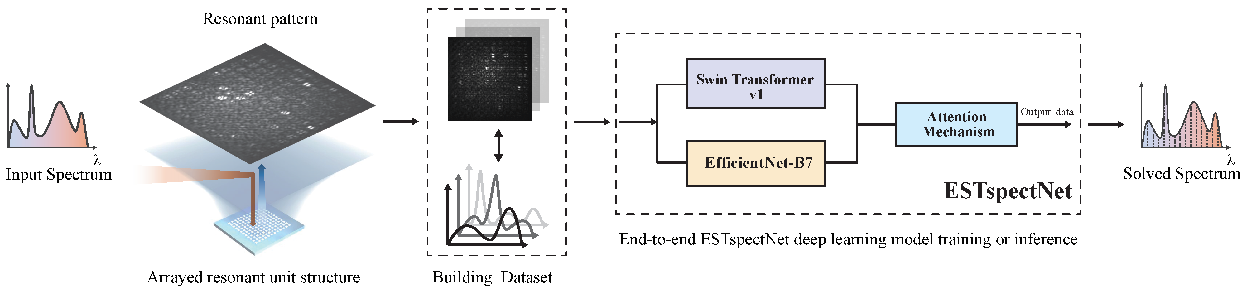
2.1. Principle of Spectrum Reconstruction Using an Array Strategy

We aim to achieve accurate spectral reconstruction through optimizing the algorithms upon snapshotting the spectral-selective response from arrayed resonators as schematically shown in Figure 1. Specifically, we work on an array whose unit elements exhibit distinct resonant responses, enabling efficient features for learning and data processing. The essence of spectral reconstruction lies in precisely recovering the incident spectral information from the array’s response signal. Such a task requires mathematical modeling and signal processing of the array data. For a typical narrowband array, its spectral response can be expressed as
R array ( r array , λ ) = f array I incident ( r array , λ ) , r array , λ ,
where I incident ( r array , λ ) represents the input spectrum at the position r array . The intensity response can be captured by a Complementary Metal-Oxide-Semiconductor (CMOS) detector, I CMOS ( r CMOS , λ ) , modeled as
I CMOS ( r CMOS , λ ) = R array ( r array , λ ) · T ( r array r CMOS ) · I incident ( r array , λ ) d r array ,
where T ( r array r CMOS ) represents the transfer function from the array elements to the CMOS detector. Conventional reconstruction methods are typically based on linear algebra or compressed sensing theory, to estimate the spectral distribution by solving the following inverse problem:
S λ = R ( I CMOS ( r CMOS , λ ) ) ,
where R ( · ) denotes the conventional reconstruction operator. However, these approaches encounter three major challenges:
  • Ill-posedness: Due to the undersampling nature of array responses, the reconstruction problem is inherently ill-posed. Conventional methods require strong regularization constraints, which may lead to the loss of spectral details.
  • Nonlinear responses: Practical systems are usually less ideal in detector’s nonlinearities and optical crosstalk. Conventional linear models struggle to accurately capture these nonlinear characteristics.
  • Noise sensitivity: Various noise sources, including CMOS readout noise and dark current noise, significantly degrade reconstruction quality. Traditional denoising methods have limitations in preserving spectral features effectively.
We propose to use a deep learning method to overcome these challenges. Through an end-to-end training process, deep learning models can automatically learn the complex nonlinear mapping between input data and output spectra, thereby reducing dependence on prior information. Deep learning also effectively captures intricate factors such as detector nonlinearities and optical crosstalk. Moreover, deep learning models extract multi-level features, significantly enhancing adaptability and generalization capability. Importantly, deep learning-based models exhibit high robustness to noise. Even under severe noise interference, they maintain high reconstruction accuracy, effectively avoiding information loss inherent in traditional denoising methods. Given these advantages, deep learning offers an efficient and reliable pathway for spectral reconstruction, paving the way for improved performance in miniature spectrometers.

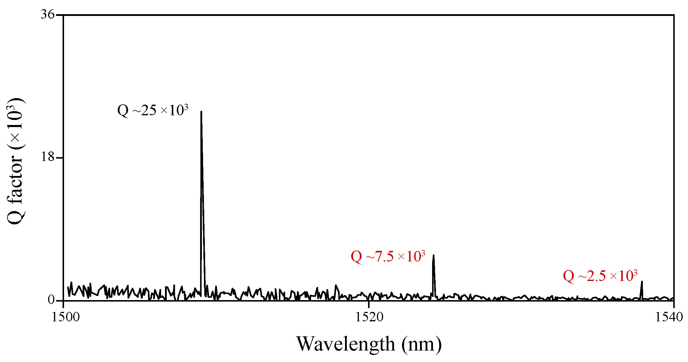
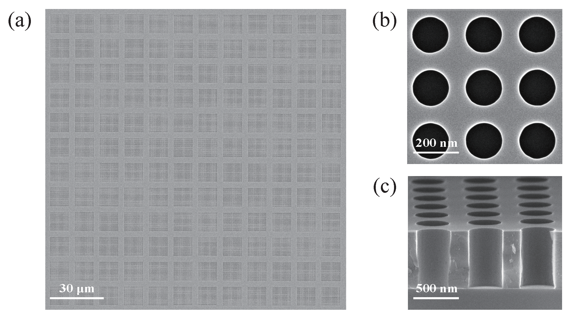
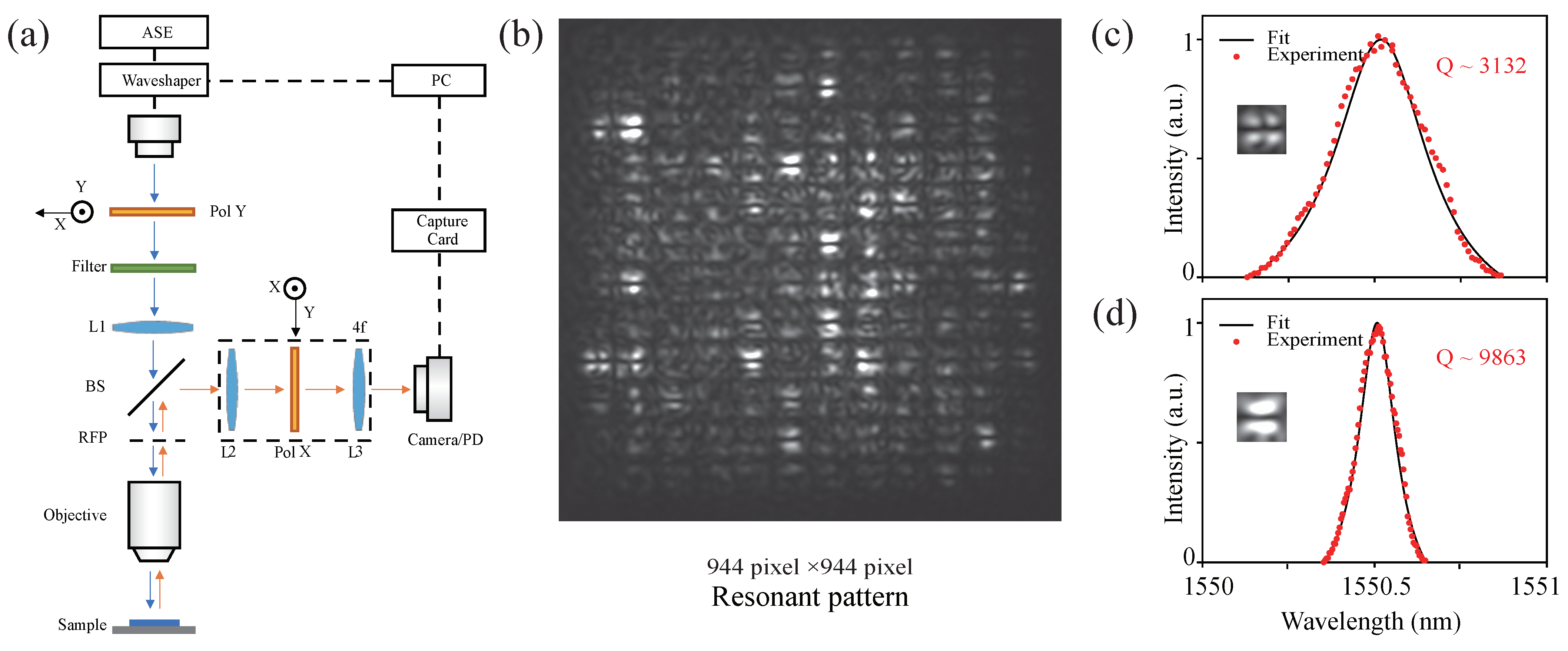
2.2. Photonic Crystal Microcavity Array: Design, Fabrication, and Testing

We further introduce our physical system cooperating with the deep learning model, which is a PhC cavity array with distinct resonance patterns at different excitation wavelengths. Specifically, we adopt miniaturized bound states in the continuum (mini-BICs) cavities with high Q-factors and rich modes as resonant units [27] for our validation. By continuously tuning the lattice constant, the cavity array can cover a wide spectral range (for details, refer to our previous work [28]). The 144-unit array features a lattice constant a = 520–539.48 nm in the core region and b = 537–561.48 nm in the boundary region, separated with gap distances g = 525–549.48 nm at 0.17 nm steps. As shown in Figure 2, numerical simulations confirm that such a silicon-on-insulator (SOI)-based cavity array achieves resonant responses with Q-factors of 7.5 × 10 3 and 2.5 × 10 3 (FWHM values of 0.6 and 0.2 nm) across the detection range.
We fabricate our sample on an SOI wafer using electron-beam lithography (EBL) and inductively coupled plasma (ICP) etching, which consists of the following processes: spin coating resist 420 nm ZEP520A, exposure to EBL (1 nA beam current, 500  μ m field size), ICP etching with SF6/CHF3 mixture, and resist removal with DMAC. As shown in Figure 3a–c, SEM images clearly display the fabricated resonator array structure with well-defined photonic crystal holes and sidewalls, confirming excellent fabrication quality.
For characterization, a tunable laser (Santec TSL-550) was employed for characterization, offering a wavelength range of 1525–1605 nm, an output power of 12 dBm, and a wavelength accuracy of 5 pm. This instrument was selected due to its precise wavelength control and stable output, qualities essential for resonant excitation. The output passes through a Y-Pol polarizer and L1 lens before 50× objective focusing. Reflected/scattered light is collected through the same objective, reduced by a 0.5× 4f system, filtered through X-Pol, and detected by a photodiode. Resonance peaks are recorded via a high-speed data acquisition card and fitted with Lorentzian functions. A flip mirror enables switching to an InGaAs CMOS camera. As illustrated in Figure 4a, an array response pattern was recorded using a CMOS camera (944 × 944 pixels). The experimental setup comprised a 5× objective, an amplified spontaneous emission (ASE) broadband source, which generates incoherent light via stimulated and spontaneous emission within a gain medium, and a programmable waveshaper. The system automatically synchronizes spectrum shaping and data acquisition for neural network training. As shown in Figure 4b–d, the measured array response clearly displays the mini-BICs modes, with experimental Qs matching well with simulations.

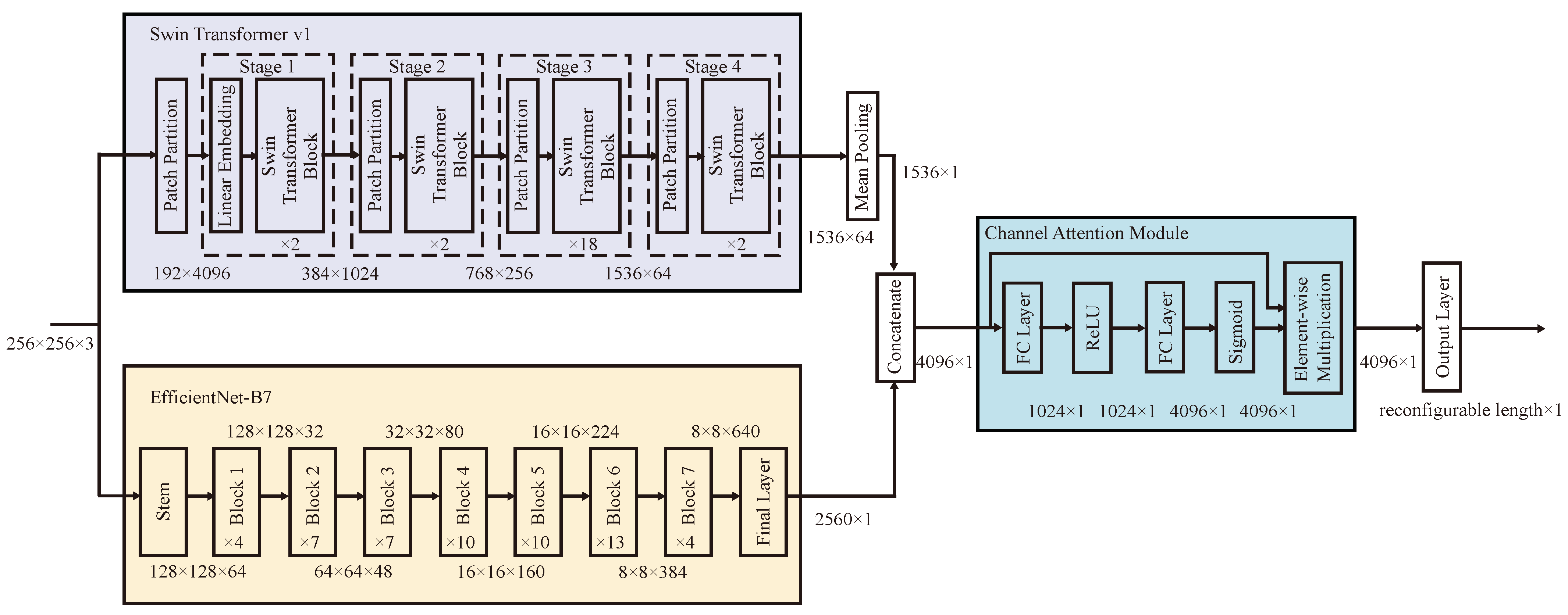
2.3. ESTspecNet: An End-to-End Learning Model for Image-to-Spectrum Reconstruction

Next, we elaborate on our end-to-end deep learning model—ESTspecNet, for image-to-spectrum reconstruction. The model integrates a multimodal feature extraction mechanism to overcome the aforementioned limitations through efficient feature learning and data processing. As shown in Figure 5, the architecture of ESTspecNet comprises an image resizing module, parallel feature extraction networks (EfficientNet-B7 and Swin Transformer v1), a channel attention mechanism, and a feature fusion layer, optimized using a composite loss function.
Initially, the cavities’ response patterns from external incident light are collected by the measurement system and serve as the network input. The input image, with a size of 944 × 944 , is resized to 256 × 256 using 3 × 3 Gaussian kernel convolution and bilinear interpolation by the image resizing module, which achieves noise smoothing and matches the pre-training input size of our model. The resized image is then fed into two parallel networks: EfficientNet-B7 and Swin Transformer v1. EfficientNet-B7, consisting of 239 MBConv layers, outputs a 2560-dimensional feature vector, while Swin Transformer v1, utilizing 12 layers of window-based multi-head self-attention modules, generates a 1536-dimensional feature vector. These networks work in parallel to extract local features and capture global dependencies, thereby enhancing the accuracy of spectral reconstruction comprehensively.
Next, in the feature fusion stage, the 2D feature map from EfficientNet-B7 is flattened and concatenated with the 1D feature vector from Swin Transformer v1, forming a joint feature vector F joint R 4096 . This joint feature vector is then weighted using the channel attention module, which operates through the following steps:
  • Dimension Compression: The first fully connected layer compresses the feature dimension from 4096 to 1024 using learnable parameters W 1 R 1024 × 4096 and b 1 R 1024 :
    z = W 1 F joint + b 1
  • Non-Linear Activation applies ReLU activation to introduce non-linearity:
    a = max ( 0 , z )
  • Dimension Expansion: The second fully connected layer restores the original dimensionality with W 2 R 4096 × 1024 and b 2 R 4096 :
    e = W 2 a + b 2
  • Adaptive Weighting generates channel-wise attention weights α [ 0 , 1 ] 4096 through sigmoid activation:
    α = σ ( e )
  • Feature Enhancement performs element-wise multiplication to obtain the final weighted features:
    F = F joint α
This bottleneck architecture (4096 → 1024 → 4096) facilitates cross-channel interaction, enabling the network to emphasize discriminative wavelength components through learned transformations defined by W 1 and W 2 . The resulting weighted feature vector, F out R 4096 , represents an enhanced spectral representation where critical components are automatically prioritized based on their wavelength-specific importance.
The weighted feature vector is mapped to the target output dimension via a fully connected layer, where the output dimension is dynamically determined by the spectral data length. In this study, the output dimension is set to 4000, corresponding to spectral data with a precision of 0.02 nm. This process effectively maps high-dimensional image features to low-dimensional spectral data, yielding accurate spectral reconstruction results.
To optimize the model, we also designed a composite loss function incorporating cosine similarity loss, mean squared error (MSE) loss, and steepness penalty, mathematically expressed as
L total = α L c o s i n e + β L mse + γ L steepness
where L total represents the total loss, L c o s i n e is the cosine similarity loss, L mse is the mean squared error loss, and L steepness is the steepness penalty. The hyperparameters α , β , and γ control the relative weights of each loss component. Their definitions are elaborated as follows:
Cosine Similarity Loss measures the angular difference between the predicted and target spectra:
L c o s i n e = 1 y · y ^ y 2 y ^ 2
where y and y ^ denote the target and predicted spectra, respectively, y 2 and y ^ 2 are their L2 norms, and y · y ^ represents their dot product, reflecting directional consistency.
MSE Loss quantifies the squared difference between the predicted and actual spectral data:
L mse = 1 N i = 1 N ( y i y ^ i ) 2
where N is the spectral data dimension, ensuring numerical consistency between the predicted and target spectra.
Steepness Penalty Loss constrains abrupt spectral variations to preserve the characteristics of narrow linewidth samples, preventing overfitting or excessive sensitivity to noise. Physically, it enforces second-order smoothness in the reconstructed spectrum by penalizing squared second derivatives of the reconstruction errors, which corresponds to constraining abrupt changes in the error gradient:
L steepness = 1 N 2 i = 2 N 1 ( y i y ^ i ) ( y i 1 y ^ i 1 ) ( y i 1 y ^ i 1 ) ( y i 2 y ^ i 2 ) 2
This composite loss function comprehensively addresses the multifaceted requirements of spectral reconstruction, ensuring spectral shape accuracy, numerical precision, and smoothness. By incorporating these mechanisms, ESTspecNet demonstrates exceptional performance in handling complex nonlinear mappings, noise interference, and high-dimensional data, offering an efficient and reliable spectral reconstruction solution.

3. Results

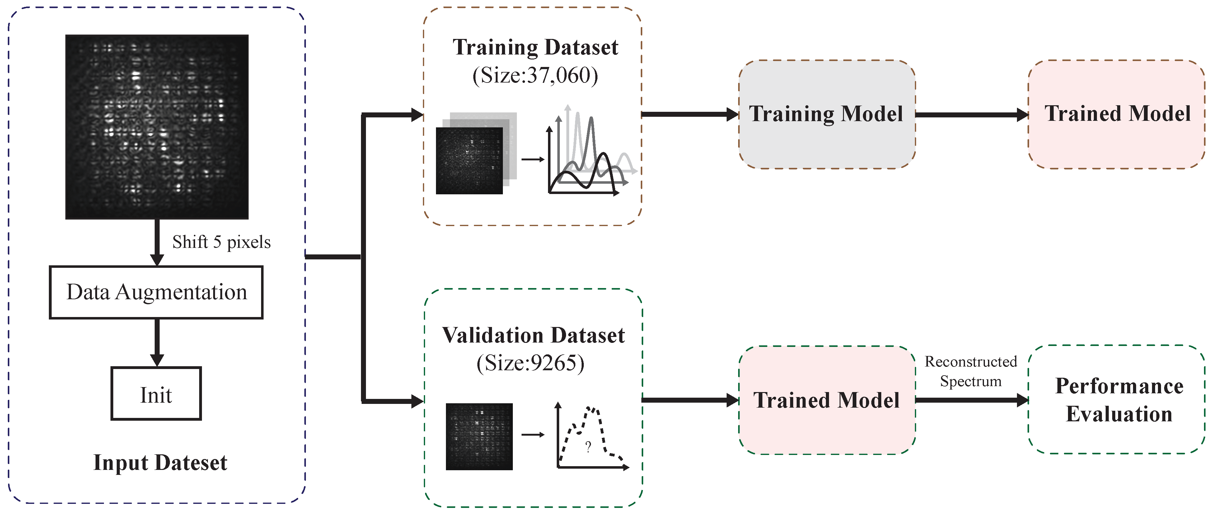
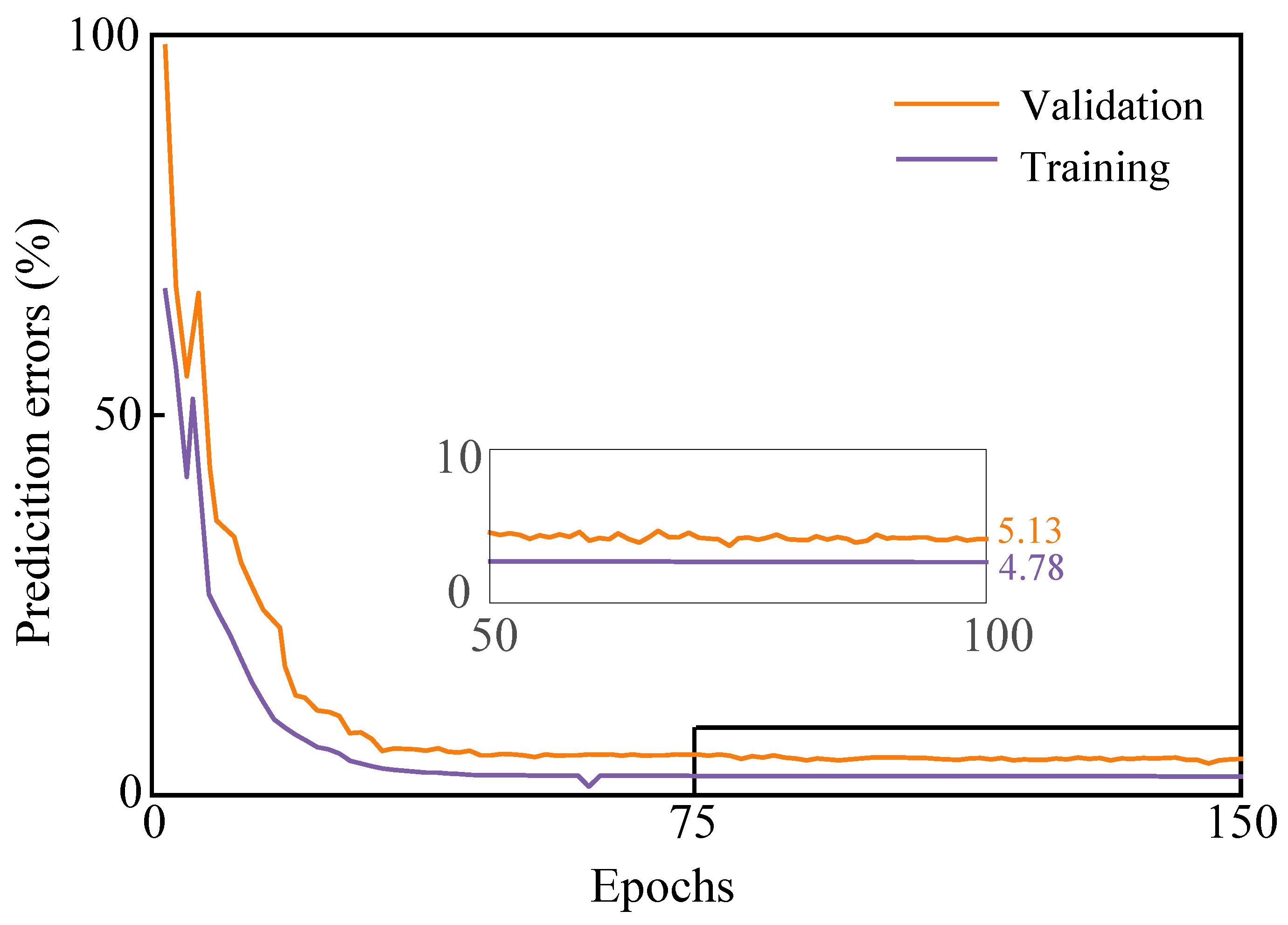
3.1. Experimental Data and Training Process

As shown in Figure 6, the training flow on the array response is depicted as follows: first, the input spectrum is recorded by a commercial spectrometer as reference, while its array response patterns are captured using a CMOS (SONY IMX990) camera, comprising a total of 9265 images with a resolution of 944 × 944 pixels. To expand the dataset, each image undergoes data augmentation via a 5-pixel translation, ultimately increasing the dataset size to 46,325. The spectral data has a length of 4000, corresponding to a measurement range of 1525–1605 nm with a spectral resolution of 0.02 nm. Among the dataset, 80% of the data are used for training and 20% for validation.
During the training phase, a mixed-precision optimization strategy (AMP) is employed to accelerate training and reduce memory consumption. The Adam optimizer is utilized with an initial learning rate of 1 × 10 4 , and a cosine annealing learning rate scheduler dynamically adjusts the learning rate to balance convergence speed and stability. The loss function consists of three components: cosine similarity loss (weight α = 0.1 ), which measures the directional consistency between the reconstructed and ground truth spectra, MSE loss (weight β = 0.9 ), which optimizes numerical precision, and a second-order difference penalty term (weight Γ = 10 ), which suppresses noise interference and prevents overfitting. The weighted combination of these losses ensures both directional consistency and numerical accuracy in spectral reconstruction. The training process runs for 150 epochs, with model performance evaluated on the validation set at the end of each epoch, and the model checkpoint with the lowest validation loss is saved.

3.2. Metrics for Evaluating Spectral Reconstruction Performance

We evaluate the model performance from two aspects: narrow-peak reconstruction ability and multi-feature peak fitting accuracy. The narrow-peak reconstruction performance can be depicted by Peak Error (PE), which measures the absolute error of narrow peaks (assumed at wavelengths λ 1 and λ 2 ), calculated as
P E k = y λ k y ^ λ k ( k = 1 , 2 )
where y λ k and y ^ λ k are the reference and reconstructed spectral intensity values at wavelength λ k , respectively. A lower PE indicates higher reconstruction accuracy of narrow peak wavelengths. Additionally, Full-Width at Half-Maximum Error (FWHM Error, FE) can assess the reconstruction accuracy of peak width, defined as
F E k = FWHM ( y λ k ) FWHM ( y ^ λ k ) ( k = 1 , 2 )
where FWHM ( · ) denotes the function for computing full-width at half-maximum. A lower FE indicates better reconstruction accuracy of peak widths.
On the other hand, multi-feature peak reconstruction performance in a wide spectrum can be described by Mean Squared Error (MSE), which measures the global numerical discrepancy between the reconstructed and actual spectra, as shown in Formula (11). Peak Signal-to-Noise Ratio (PSNR) evaluates the overall fidelity of spectral waveforms, as follows:
P S N R = 10 log 10 M A X 2 M S E
where M A X is the maximum intensity value of the spectral data. A higher PSNR indicates lower noise in the reconstructed spectrum. Additionally, the Structural Similarity Index (SSIM) assesses the structural similarity between spectral waveforms:
S S I M = 2 μ y μ y ^ + C 1 2 σ y y ^ + C 2 μ y 2 + μ y ^ 2 + C 1 σ y 2 + σ y ^ 2 + C 2
where μ y and μ y ^ are the mean values of the actual and reconstructed spectra, σ y and σ y ^ are their standard deviations, σ y y ^ represents covariance, and C 1 and C 2 are constants. An SSIM value closer to 1 indicates higher structural similarity between the reconstructed and actual spectra.

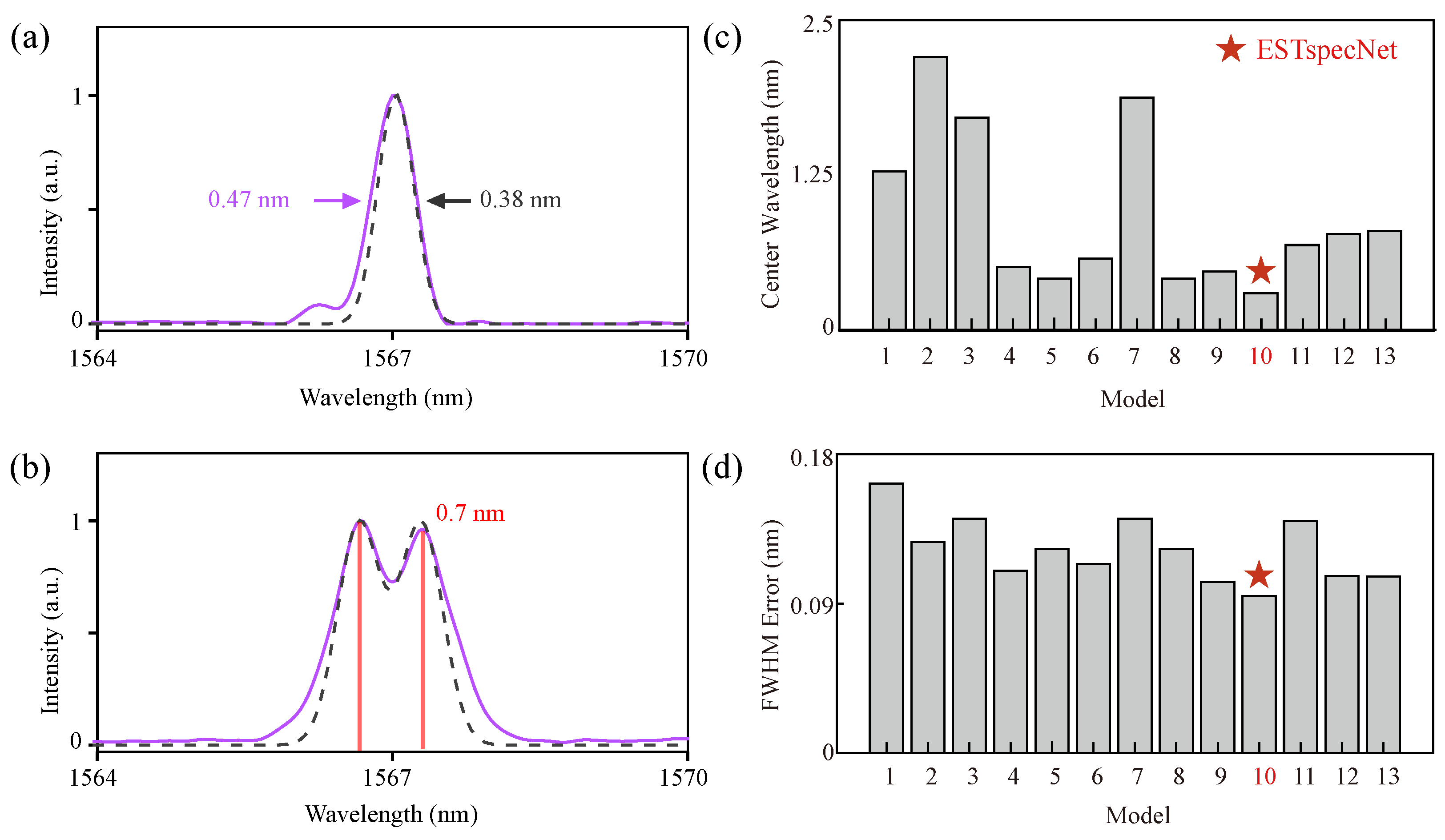
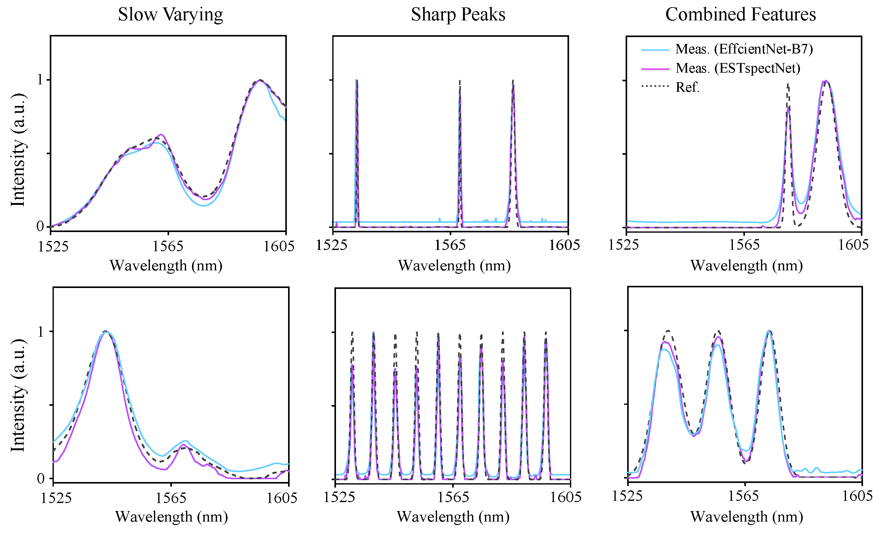
3.3. Model Performance and Analysis

To comprehensively evaluate the performance of different models, we implemented a progressive experiment. Baseline models encompassed three modules: EfficientNet-B7, ResNet, and Swin Transformer, each trained under two conditions, namely without data augmentation (baseline group) and with 5-pixel shift augmentation. In further experiments, attention mechanisms were induced, and the effectiveness of different model combinations was explored, including single-model configurations, dual-model fusion, and triple-model fusion, with specific model combinations and identifiers detailed in Table 1. Model performance was evaluated based on the metrics mentioned above—MSE, PSNR, and SSIM, along with FWHM error and central wavelength λ c error.

3.4. Model Performance Comparison

The results presented in Table 2 reveal some differences across the models. Swin Transformer outperforms ResNet in terms of MSE and SSIM under non-augmented conditions. This advantage stems from its hierarchical attention mechanism, where the shifting window strategy allows for cross-window global dependency modeling, whereas Model 2’s (ResNet-50) residual blocks are constrained by the local receptive field of 3 × 3 convolutions. Notably, Model 3 (Swin Transformer) exhibits a central wavelength error of only 1.71 nm, lower than EfficientNet’s performance. This could be attributed to the pure attention mechanism’s relative insensitivity to spatial localization. EfficientNet, leveraging compound scaling to balance depth, width, and resolution, benefits from its progressive downsampling strategy, which is advantageous for coordinating regression tasks.

3.5. Impact of Data Augmentation

To investigate the impact of data augmentation, the dataset is enlarged 5 times by shifting the images by 5 pixels in four directions. Table 2 compares single-model performance before and after augmentation. The results indicate that data augmentation significantly improves model performance.
After augmentation, EfficientNet’s MSE decreases by 23.13% and central wavelength error reduces by 60.42%, demonstrating its ability to learn more robust features. ResNet’s MSE increases slightly by 0.2%, yet PSNR improves by 0.83 dB. This suggests that, while MSE is sensitive to global errors, PSNR prioritizes peak signal fidelity—ResNet may have learned enhanced peak detection capabilities (reducing central wavelength error by 81.28%) but at the cost of overall reconstruction precision. This phenomenon highlights architectural limitations in spectral reconstruction tasks. Swin Transformer also benefits from augmentation, reducing FWHM error by 19.46%, indicating that its hierarchical attention mechanism effectively utilizes augmented data.

3.6. Effect of Attention Mechanism

Applying attention mechanisms shows distinct performance across models, as evidenced in Table 3. While ResNet-based implementations (Model 8) show negligible MSE variation and a stable PSNR, both EfficientNet (Model 7) and Swin Transformer (Model 9) exhibit performance degradation upon attention module insertion. Specifically, EfficientNet suffers a 4.78% MSE increase coupled with 0.94 dB PSNR reduction, while Swin Transformer demonstrates a more pronounced 7.29% MSE deterioration and 0.47 dB PSNR decline. This divergence stems from fundamental architectural characteristics: EfficientNet’s inherent Mobile Inverted Bottleneck (MBConv) layers already integrate Squeeze-and-Excitation (SE) attention for channel-wise feature recalibration. Additional attention modules create conflicting channel weighting priorities, particularly in spectral background regions where redundant activation patterns increase reconstruction noise.
Conversely, Swin Transformer’s performance degradation arises from positional encoding conflicts—the base architecture employs absolute positional embeddings, while the supplementary attention module utilizes relative positional encoding. This mismatch induces phase alignment errors in high-frequency spectral components, evidenced by a 23% increase in reconstruction error for spectral peaks where FWHM < 0.15 nm. The results demonstrate that attention mechanisms require careful architectural co-design rather than naive module insertion.

3.7. Analysis of Model Fusion Strategies

The evaluation in Table 4 recognizes ESTspecNet (Model 10) as the optimal fusion strategy, achieving state-of-the-art performance across all critical metrics. With a central wavelength error of 0.29 nm, ESTspecNet demonstrates 57.29% improvement over the ResNet+EfficientNet ensemble (Model 11) and 63.16% superiority to the ResNet+Swin combination (Model 12). This performance advantage originates from the complementary strengths of its constituent architectures: Swin Transformer’s global dependency modeling capability, evidenced by its 0.943 SSIM in baseline measurements (Table 2), synergizes with EfficientNet’s localized precision reflected in 1.27 nm native λ c accuracy. The fusion mechanism effectively balances these attributes through learned attention gates.
Technically, the proposed ESTspecNet is implemented using the PyTorch 2.3.1 framework, trained and validated on an NVIDIA H20 GPU. To balance memory consumption and training efficiency, the batch size is set to 32. Mixed-precision training is employed via PyTorch’s torch.cuda.amp module, with gradient scaling managed by GradScaler. The cosine annealing learning rate scheduler is configured with a minimum learning rate of 1 × 10 6 and a cycle length of 150 epochs. As shown in Figure 7, the training dynamics confirm its stability, with prediction errors for both the training dataset (purple curve) and the test dataset (orange curve) decreasing to below 6%.
To further assess the spectral reconstruction capability in detail, particularly in terms of narrow peak restoration and reconstruction performance, Figure 8a,b presents the average λ c e n t e r error and FWHM error for the 13 model combinations in single-peak reconstruction. The results indicate that the single-peak resolution achieved by the ESTspecNet-based reconstructed spectrum is 0.47 nm, while the double-peak resolution reaches 0.7 nm, demonstrating superior resolution performance (Figure 8c,d). Additionally, spectral reconstruction using a single EfficientNet model achieves a single-peak resolution of 0.55 nm and a double-peak resolution of 0.8 nm. These findings confirm that ESTspecNet improves narrow peak resolution by more than 10%. Specifically, the central wavelength error of ESTspecNet is 0.29 nm, representing an 82.98% reduction compared to the baseline Swin Transformer, while the FWHM error is 0.09 nm, showing an 18.18% improvement over the data-enhanced version of EfficientNet.
We explain that the superior performance of this approach primarily stems from its multi-scale feature extraction, efficient feature fusion, and enhanced robustness. By integrating the compound scaling mechanism of EfficientNet with the hierarchical attention mechanism of the Swin Transformer, the model effectively captures both local details and the global structure of spectral signals, particularly when addressing complex spectral peak overlap issues.
Finally, the reconstruction performance and physical consistency of the model were further validated. As illustrated in Figure 9, the reconstruction results for slowly varying spectra, multi-peak spectra, and fused spectral profiles are presented, based on both the EfficientNet-B7 baseline and the proposed ESTspecNet model. The blue curves represent the reconstruction outputs of the EfficientNet-B7 model, while the purple curves correspond to those of ESTspecNet. The results confirm that ESTspecNet exhibits excellent reconstruction performance in terms of both peak shape fidelity and signal-to-noise ratio, consistently outperforming the baseline across various spectral types. These findings support the model’s enhanced capability to accurately recover the physical characteristics of real-world spectra in practical sensing scenarios.

4. Discussion and Conclusions

The major challenge in parallel detection of spectral-selective resonator arrays lies in coordinating a large number of resonant elements, where precise fabrication and calibration present significant technical barriers [29,30]. End-to-end deep learning optimization strategies offer an innovative solution—leveraging data-driven deep network training paradigms [31,32,33] enables implicit modeling of the complex responses across massive resonant units, circumventing the dependence on prior physical models inherent in traditional methods.
In this study, we propose an architecture with adaptability for spectral reconstruction tailored to general resonator arrays. By constructing a hybrid convolution-attention feature extraction module, our approach achieves synergistic perception of both local perturbation features and global correlation patterns. Integrating a physics-constrained loss function with a dynamic weight optimization strategy, the method effectively addresses key challenges, including inter-channel crosstalk, nonlinear feature superposition, and unit response coupling in large-scale arrays. This approach not only preserves physical interpretability but also attains sub-nanometer spectral reconstruction accuracy.
Experimental results demonstrate that, for single-peak reconstruction tasks in the near-infrared range (80 nm bandwidth), our model reduces the central wavelength error to 0.29 nm, achieving an 82.4% improvement over baseline models, while optimizing the FWHM error to 0.09 nm, representing a relative enhancement of 18.18%. The current resolution limitation primarily arises from the Q-factor of the resonant units and the array scale. However, optimizing unit design and expanding the array dimensions can effectively overcome this bottleneck.
While offering substantial performance improvements, this approach presents computational challenges that scale with increasing complexity. The high-Q nature of the resonant units also highlights the importance of precise temperature control to minimize wavelength drift; active stabilization or periodic recalibration may be required in certain environments. Our model’s adaptable architecture and modular design offer promising avenues for future research into transfer learning techniques, which could potentially reduce the need for full retraining when applied to novel resonator geometries such as plasmonic or dielectric metasurfaces.
Notably, the proposed method exhibits strong compatibility with wavelength-selective materials (e.g., quantum dots [12]) and its modular design supports rapid adaptive training across diverse resonant array architectures, laying a critical foundation for intelligent spectral sensing systems. To address scalability challenges, future work will explore distributed training across multiple devices to alleviate computational burdens.
Beyond restoring real spectral properties with high fidelity, ESTspecNet provides a novel framework for deep learning in spectral analysis. Its broad applicability to spectral detection micro-nanostructures makes it a key enabler for next-generation intelligent spectral sensor chips, with strong potential for high-density integration and real-time applications.

Author Contributions

X.Z., C.Z. and C.P. conceived the idea for this work. C.Z., H.L. and C.P. supervised the research. X.Z. was responsible for the design of the devices and fabricated the sample. X.Z. and C.Z. built the measurement system and conducted experimental measurements. X.Z., C.Z. and Z.Z. performed data processing and analysis. All of the authors discussed the results and contributed to the preparation of the manuscript and discussions. All authors have read and agreed to the published version of the manuscript.

Funding

This work was partly supported by the National Key Research and Development Program of China (2022YFA1404804 and 2023YFB2905501) and the National Natural Science Foundation of China (No. 62325501 and No. 62135001). The simulation of this work was supported by High-Performance Computing Platform of Peking University.

Institutional Review Board Statement

Not applicable.

Informed Consent Statement

Not applicable.

Data Availability Statement

The data supporting this study’s findings are available from the corresponding author upon reasonable request.

Conflicts of Interest

The authors declare that there are no conflicts of interest.

Abbreviations

The following abbreviations are used in this manuscript:
Qquality factor
MLmachine learning
mini-BICsminiaturized bound states in the continuum
ASEamplified spontaneous emission
SOIsilicon-on-insulator
ICPinductively coupled plasma
EBLelectron beam lithography
SNRsignal-to-noise ratios
MBConvmobile inverted bottleneck convolution
CNNsconvolutional neural networks
DNNsdeep neural networks
SEsqueeze-and-excitation
MSEmean square error
FWHMfull width at half maximum
PSNRPeak Signal-to-Noise Ratio
SSIMStructural Similarity Index
PEPeak error
FEfull width at half maximum error
CMOSComplementary Metal-Oxide-Semiconductor

References

  1. Babos, D.V.; Tadini, A.M.; De Morais, C.P.; Barreto, B.B.; Carvalho, M.A.; Bernardi, A.C.; Oliveira, P.P.; Pezzopane, J.R.; Milori, D.M.; Martin-Neto, L. Laser-induced breakdown spectroscopy (LIBS) as an analytical tool in precision agriculture: Evaluation of spatial variability of soil fertility in integrated agricultural production systems. Catena 2024, 239, 107914. [Google Scholar] [CrossRef]
  2. Barulin, A.; Kim, Y.; Oh, D.K.; Jang, J.; Park, H.; Rho, J.; Kim, I. Dual-wavelength metalens enables Epi-fluorescence detection from single molecules. Nat. Commun. 2024, 15, 26. [Google Scholar] [CrossRef] [PubMed]
  3. Li, A.; Yao, C.; Xia, J.; Wang, H.; Cheng, Q.; Penty, R.; Fainman, Y.; Pan, S. Advances in cost-effective integrated spectrometers. Light. Sci. Appl. 2022, 11, 174. [Google Scholar] [CrossRef]
  4. Calafiore, G.; Koshelev, A.; Dhuey, S.; Goltsov, A.; Sasorov, P.; Babin, S.; Yankov, V.; Cabrini, S.; Peroz, C. Holographic planar lightwave circuit for on-chip spectroscopy. Light. Sci. Appl. 2014, 3, e203. [Google Scholar] [CrossRef]
  5. Zheng, S.; Cai, H.; Song, J.; Zou, J.; Liu, P.Y.; Lin, Z.; Kwong, D.L.; Liu, A.Q. A single-chip integrated spectrometer via tunable microring resonator array. IEEE Photonics J. 2019, 11, 1–9. [Google Scholar] [CrossRef]
  6. Kita, D.M.; Miranda, B.; Favela, D.; Bono, D.; Michon, J.; Lin, H.; Gu, T.; Hu, J. High-performance and scalable on-chip digital Fourier transform spectroscopy. Nat. Commun. 2018, 9, 4405. [Google Scholar] [CrossRef]
  7. Zheng, Q.; Nan, X.; Chen, B.; Wang, H.; Nie, H.; Gao, M.; Liu, Z.; Wen, L.; Cumming, D.R.; Chen, Q. On-Chip Near-Infrared Spectral Sensing with Minimal Plasmon-Modulated Channels. Laser Photonics Rev. 2023, 17, 2300475. [Google Scholar] [CrossRef]
  8. Yang, Z.; Albrow-Owen, T.; Cui, H.; Alexander-Webber, J.; Gu, F.; Wang, X.; Wu, T.C.; Zhuge, M.; Williams, C.; Wang, P.; et al. Single-nanowire spectrometers. Science 2019, 365, 1017–1020. [Google Scholar] [CrossRef]
  9. Lin, X.; Wang, W.; Zhao, Y.; Yan, R.; Li, J.; Chen, H.; Lu, G.; Liu, F.; Du, G. High-accuracy direction measurement and high-resolution computational spectral reconstruction based on photonic crystal array. Opt. Express 2024, 32, 36085–36092. [Google Scholar] [CrossRef]
  10. Wang, Z.; Yi, S.; Chen, A.; Zhou, M.; Luk, T.S.; James, A.; Nogan, J.; Ross, W.; Joe, G.; Shahsafi, A.; et al. Single-shot on-chip spectral sensors based on photonic crystal slabs. Nat. Commun. 2019, 10, 1020. [Google Scholar] [CrossRef]
  11. Zhao, D.; Shao, H.; Zheng, Y.; Xu, Y.; Bao, J. Dual-layer broadband encoding spectrometer: Enhanced encoder basis orthogonality and spectral detection accuracy. Opt. Express 2024, 32, 39222–39244. [Google Scholar] [CrossRef] [PubMed]
  12. Zhu, X.; Bian, L.; Fu, H.; Wang, L.; Zou, B.; Dai, Q.; Zhang, J.; Zhong, H. Broadband perovskite quantum dot spectrometer beyond human visual resolution. Light. Sci. Appl. 2020, 9, 73. [Google Scholar] [CrossRef] [PubMed]
  13. Zhou, J.; Al Husseini, D.; Li, J.; Lin, Z.; Sukhishvili, S.; Cote, G.L.; Gutierrez-Osuna, R.; Lin, P.T. Mid-Infrared Serial Microring Resonator Array for Real-Time Detection of Vapor-Phase Volatile Organic Compounds. Anal. Chem. 2022, 94, 11008–11015. [Google Scholar] [CrossRef] [PubMed]
  14. Chen, X.; Gan, X.; Zhu, Y.; Zhang, J. On-chip micro-ring resonator array spectrum detection system based on convex optimization algorithm. Nanophotonics 2023, 12, 715–724. [Google Scholar] [CrossRef]
  15. Guan, Q.; Lim, Z.H.; Sun, H.; Chew, J.X.Y.; Zhou, G. Review of miniaturized computational spectrometers. Sensors 2023, 23, 8768. [Google Scholar] [CrossRef]
  16. Björck, Å. Least squares methods. Handb. Numer. Anal. 1990, 1, 465–652. [Google Scholar]
  17. Oliver, J.; Lee, W.; Park, S.; Lee, H.N. Improving resolution of miniature spectrometers by exploiting sparse nature of signals. Opt. Express 2012, 20, 2613–2625. [Google Scholar] [CrossRef]
  18. Wang, W.; Dong, Q.; Zhang, Z.; Cao, H.; Xiang, J.; Gao, L. Inverse design of photonic crystal filters with arbitrary correlation and size for accurate spectrum reconstruction. Appl. Opt. 2023, 62, 1907–1914. [Google Scholar] [CrossRef]
  19. LeCun, Y.; Bengio, Y.; Hinton, G. Deep learning. Nature 2015, 521, 436–444. [Google Scholar] [CrossRef]
  20. Silver, D.; Hasselt, H.; Hessel, M.; Schaul, T.; Guez, A.; Harley, T.; Dulac-Arnold, G.; Reichert, D.; Rabinowitz, N.; Barreto, A.; et al. The predictron: End-to-end learning and planning. In Proceedings of the International Conference on Machine Learning, PMLR, Sydney, Australia, 6–11 August 2017; pp. 3191–3199. [Google Scholar]
  21. Chen, J.; Li, P.; Wang, Y.; Ku, P.C.; Qu, Q. Sim2Real in reconstructive spectroscopy: Deep learning with augmented device-informed data simulation. APL Mach. Learn. 2024, 2, 036106. [Google Scholar] [CrossRef]
  22. Alzubaidi, L.; Zhang, J.; Humaidi, A.J.; Al-Dujaili, A.; Duan, Y.; Al-Shamma, O.; Santamaría, J.; Fadhel, M.A.; Al-Amidie, M.; Farhan, L. Review of deep learning: Concepts, CNN architectures, challenges, applications, future directions. J. Big Data 2021, 8, 1–74. [Google Scholar]
  23. Tan, M.; Le, Q. EfficientNet: Rethinking Model Scaling for Convolutional Neural Networks. In Proceedings of the 36th International Conference on Machine Learning, PMLR, Long Beach, CA, USA, 9–15 June 2019; pp. 6105–6114. [Google Scholar]
  24. Wang, J.; Zhang, F.; Zhou, X.; Shen, X.; Niu, Q.; Yang, T. Miniaturized spectrometer based on MLP neural networks and a frosted glass encoder. Opt. Express 2024, 32, 30632–30641. [Google Scholar] [CrossRef] [PubMed]
  25. Sun, B.; Wu, C.; Yu, M. Spectral Reconstruction for Internet of Things Based on Parallel Fusion of CNN and Transformer. IEEE Internet Things J. 2024, 12, 3549–3562. [Google Scholar] [CrossRef]
  26. Guo, M.H.; Xu, T.X.; Liu, J.J.; Liu, Z.N.; Jiang, P.T.; Mu, T.J.; Zhang, S.H.; Martin, R.R.; Cheng, M.M.; Hu, S.M. Attention mechanisms in computer vision: A survey. Comput. Vis. Media 2022, 8, 331–368. [Google Scholar] [CrossRef]
  27. Chen, Z.; Yin, X.; Jin, J.; Zheng, Z.; Zhang, Z.; Wang, F.; He, L.; Zhen, B.; Peng, C. Observation of miniaturized bound states in the continuum with ultra-high quality factors. Sci. Bull. 2022, 67, 359–366. [Google Scholar] [CrossRef]
  28. Zhou, X.; Zhang, C.; Zhang, X.; Zuo, Y.; Zhang, Z.; Wang, F.; Chen, Z.; Li, H.; Peng, C. Miniaturized spectrometer enabled by end-to-end deep learning on large-scale radiative cavity array. arXiv 2024, arXiv:2411.13353. [Google Scholar]
  29. Peng, J.; Nie, W.; Li, T.; Xu, J. An end-to-end DOA estimation method based on deep learning for underwater acoustic array. In Proceedings of the OCEANS 2022, Hampton Roads, VA, USA, 17–20 October 2022; pp. 1–6. [Google Scholar]
  30. Gupta, A.; Mishra, R.; Zhang, Y. SenGLEAN: An End-to-End Deep Learning Approach for Super-Resolution of Sentinel-2 Multiresolution Multispectral Images. IEEE Trans. Geosci. Remote Sens. 2024, 62, 1–19. [Google Scholar] [CrossRef]
  31. Signoroni, A.; Savardi, M.; Baronio, A.; Benini, S. Deep Learning Meets Hyperspectral Image Analysis: A Multidisciplinary Review. J. Imaging 2019, 5, 52. [Google Scholar] [CrossRef]
  32. Gao, L.; Qu, Y.; Wang, L.; Yu, Z. Computational spectrometers enabled by nanophotonics and deep learning. Nanophotonics 2022, 11, 2507–2529. [Google Scholar] [CrossRef]
  33. Zhang, J.; Zhu, X.; Bao, J. Solver-informed neural networks for spectrum reconstruction of colloidal quantum dot spectrometers. Opt. Express 2020, 28, 33656. [Google Scholar] [CrossRef]
Figure 1. The architecture of spectral reconstruction based on end-to-end learning model, ESTspecNet.
Photonics 12 00449 g001
Figure 2. Simulation results of the response of a single mini-BICs microcavity.
Photonics 12 00449 g002
Figure 3. Scanning electron microscopy (SEM) images. (a) Fabricated mini-BICs cavity array. (b,c) Side view of the etched pores of mini-BICs cavity.
Photonics 12 00449 g003
Figure 4. Measurement systems and results. (a) Schematic of the measurement setup; (b) Typical CMOS image illustrating the spatial signature of the cavity array when the input wavelength coincides with the resonance. (c,d) Pattern of modes and measured reflection spectrum.
Photonics 12 00449 g004
Figure 5. Schematic and detailed parameter settings of the ESTspecNet model.
Photonics 12 00449 g005
Figure 6. Training and validating flow of spectrum reconstruction based on the input of array responses.
Photonics 12 00449 g006
Figure 7. Training sequence of the ESTspecNet model. The evolution of prediction error for training (purple) and validation (orange) datasets during iteration. Insets: the details after 50 iteration steps, showing that the training converges to the prediction errors.
Photonics 12 00449 g007
Figure 8. Comparison of performance metrics between ESTspecNet and other fusion model combinations. (a) Single-peak reconstruction results based on ESTspecNet. (b) Double-peak reconstruction results based on ESTspecNet. (c) Comparison of average central wavelength errors of 13 model combinations. (d) Comparison of average FWHM errors of 13 model combinations.
Photonics 12 00449 g008
Figure 9. Results of spectral reconstruction. ESTspecNet (purple) closely matches the reference spectra (black dashed), outperforming the baseline EfficientNet-B7 (blue) across all feature types: slow variations, sharp peaks, and combined features.
Photonics 12 00449 g009
Table 1. Model configurations for progressive spectral reconstruction experiments.
Model IDArchitectureTraining Configuration
Model 1EfficientNet-B7(baseline)
Model 2ResNet-50
Model 3Swin Transformer
Model 4EfficientNet-B7+ data augmentation
Model 5ResNet-50
Model 6Swin Transformer
Model 7EfficientNet-B7+ Attention + data augmentation
Model 8ResNet-50
Model 9Swin Transformer
Model 10EfficientNet-B7 + ResNet-50+ Attention + data augmentation
Model 11EfficientNet-B7 + Swin Transformer
Model 12ResNet-50 + Swin Transformer
Model 13EfficientNet-B7 + ResNet-50 + Swin Transformer+ Attention + data augmentation
Table 2. Single model performance comparison.
ModelMSE ( 10 3 )PSNR (dB)SSIM λ c Error (nm)FWHM Error (nm)
Model 15.330.390.9241.270.16
Model 24.331.570.9312.190.13
Model 34.231.880.9431.710.14
Model 44.131.910.9480.500.11
Model 54.532.400.9380.410.12
Model 64.032.460.9500.570.11
Table 3. Attention mechanism introduces performance comparison.
ModelMSE ( 10 3 )PSNR (dB)SSIM λ c Error (nm)FWHM Error (nm)
Model 74.3131.490.9441.8670.14
Model 84.5332.400.9380.410.12
Model 94.3231.990.9390.460.10
Table 4. Model fusion performance comparison.
ModelMSE ( 10 3 )PSNR (dB)SSIM λ c Error (nm)FWHM Error (nm)
Model 104.0132.630.950.290.09
Model 114.6731.360.9380.680.14
Model 124.8531.420.9340.770.11
Model 134.6431.120.9320.790.11
* Model 10 is the ESTspecNet proposed in this paper.
Disclaimer/Publisher’s Note: The statements, opinions and data contained in all publications are solely those of the individual author(s) and contributor(s) and not of MDPI and/or the editor(s). MDPI and/or the editor(s) disclaim responsibility for any injury to people or property resulting from any ideas, methods, instructions or products referred to in the content.

