Circuit-QED for Multi-Loop Fluxonium-Type Qubits

Abstract

Fluxonium qubits, designed to mitigate charge noise and enhance anharmonicity, are among the most promising superconducting platforms for quantum computing. To understand and exploit their quantum properties and design novel fluxonium-based architectures with improved functionalities, these systems require an accurate Hamiltonian formulation to capture their energy level structure and quantum dynamics. This work presents a systematic method for constructing the Hamiltonian for multi-loop circuits that partitions the system into a set of uncoupled harmonic oscillators and a coupled anharmonic part originating from the Josephson circuit elements, allowing clear identification of independent modes and isolating the nonlinearity in the Josephson terms. While demonstrated for fluxonium-type multi-loop circuits, this method can be generalized to other superconducting qubit architectures within the broader context of circuit QED, making it a versatile tool for exploring different circuit configurations. Our systematic and flexible modeling approach forms the theoretical basis for the qubit measurement and control experiments validating multi-loop fluxonium architectures.

1. Introduction

Superconducting qubits have become a leading platform for quantum computing due to their balance of flexibility, performance, and scalability enabled by established microfabrication techniques. They are well-suited for quantum gate operations, including both single and two-qubit gates and precise state readout, essential for implementing quantum algorithms. Additionally, these qubits offer excellent addressability, allowing individual qubits to be controlled and measured with high precision using microwave pulses [1,2,3,4,5].

However, the stability and performance of superconducting qubits depend strongly on their circuit architecture. Key properties such as anharmonicity, noise resilience, and coupling strength determine how well a qubit maintains coherence and executes precise quantum operations. Different qubit designs address decoherence sources (including charge, flux, and dielectric noise) in various ways: for instance, transmon qubits focus on reducing charge noise, while fluxonium qubits mitigate both charge and flux noise [6,7].

Superconducting qubits, when coupled with quantum resonators, enable measurement and control of qubit states via resonator-mediated interactions. This forms the foundation of circuit quantum electrodynamics (circuit QED), the superconducting analog of traditional cavity QED [8]. While cavity QED explores interactions between atoms and optical photons confined in a cavity, circuit QED adapts this to the microwave domain, with superconducting circuits acting as artificial atoms and resonators as microwave cavities [9]. This allows for strong light–matter interactions at gigahertz frequencies, usually using a coplanar waveguide or a 3D cavity [10,11].

Among the different types of superconducting qubits, the fluxonium qubit is one of the most promising architectures, offering high anharmonicity, improved coherence, and control properties [12,13,14,15,16,17,18,19,20,21,22,23,24,25]. To overcome charge noise sensitivity and the limited anharmonicity (encountered in charge qubits), fluxonium was designed with a large inductive shunt. Since standard inductors cannot provide sufficiently high inductance, fluxonium uses a Josephson junction array, known as a superinductor, to achieve this [26]. This design preserves strong Josephson nonlinearity while suppressing charge noise by shifting the qubit’s primary variable from charge to flux, making it tunable via external magnetic flux ${\varphi }_{ext\left(i\right)}$, denoted ${\varphi }_{e_i}$ throughout this text for simplicity. However, as for all superconducting qubits, fluxonium remains vulnerable to stability issues from external flux fluctuations and other environmental noise that cause decoherence. Alternative multi-loop architectures have been proposed to address stability-related challenges [27,28].

Before experimentally exploring these novel architectures and their properties, it is essential to first understand their energy level structures and dynamics at a theoretical level. This is achieved through circuit QED, which provides a framework for modeling quantum behavior in superconducting circuits and analyzing how these systems interact with electromagnetic fields. For multi-loop fluxonium qubits, it is especially useful to decompose the circuit into two distinct parts: one that consists of uncoupled harmonic oscillators and another that contains the coupled, nonlinear elements (the Josephson junctions). This separation allows for a clearer theoretical understanding of the system’s behavior. The harmonic part can be treated exactly, while the nonlinear Josephson terms (responsible for the system’s anharmonicity) can be addressed either perturbatively, if the nonlinearity is weak, or numerically, by representing the system in a truncated Hilbert space, often constructed from the eigenstates of the harmonic oscillators (Fock basis).

This tutorial provides a detailed introduction to the theoretical analysis of fluxonium-type circuits, especially for newcomers aiming to design qubits. This structured approach allows for a rigorous analysis of the system’s energy spectrum and dynamical properties. The focus of this tutorial is solely on the theoretical analysis of superconducting circuits, thus the experimental fabrication and implementation aspects are not covered but can be reviewed in Refs. [6,14,26,29,30,31,32,33]. This tutorial is intended as a stepping stone for readers before exploring more advanced literature [1,34,35,36,37,38,39,40], particularly for those interested in the theoretical foundations necessary to study and analyze fluxonium-type qubits. By providing a robust theoretical foundation, our method initiates the way for optimizing qubit design, enhancing coherence properties and improving the overall performance of high impedance architectures.

The paper is organized as follows: In Section 2.1, the focus is on presenting the multi-loop fluxonium circuit, detailing its structure and how to choose independent variables that effectively describe its behavior. This includes identifying the relevant node and branch flux variables and introducing a method for selecting a minimal and efficient set of variables that simplifies analysis. Section 2.2 develops the Lagrangian formulation of the system in terms of energy contributions from capacitive, inductive, and Josephson elements. Section 2.3 explains how redistributing external fluxes is done, in order to remove them from the inductive terms and move them entirely into the Josephson junction contributions, simplifying the circuit’s mathematical representation. Section 2.4 introduces the Hamiltonian formulation and redefining the coordinates that decouple the system into normal modes setting up a basis for numerical calculations and experimental investigation.

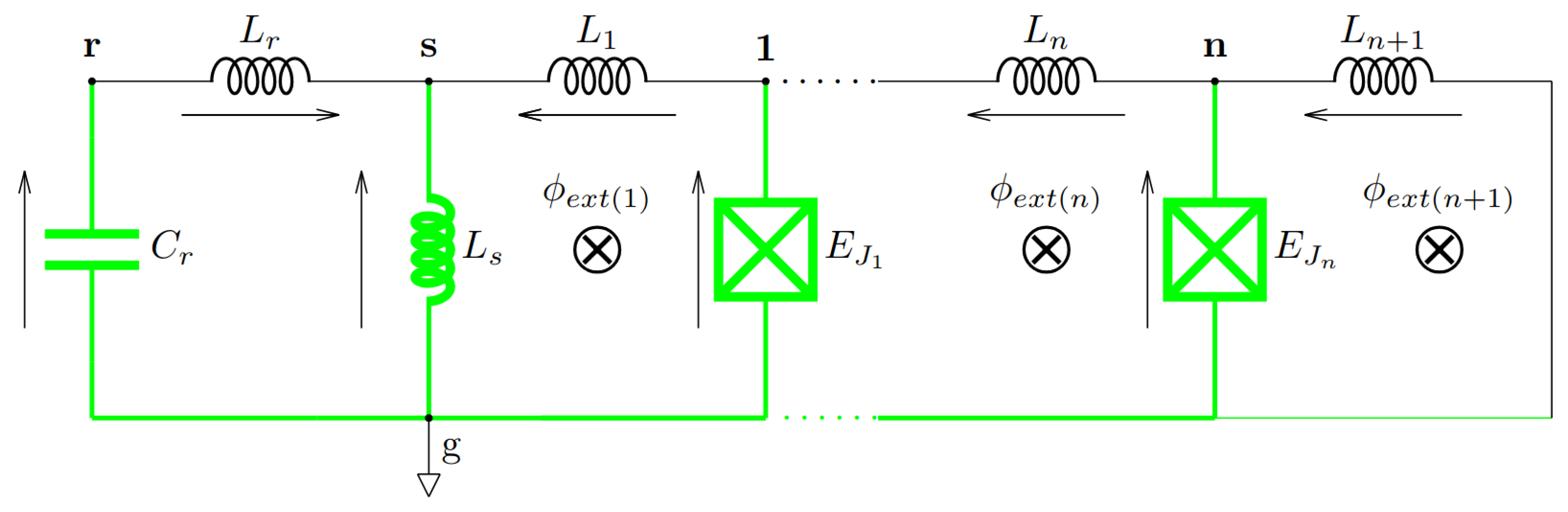
2. Multi-Loop Fluxonium

2.1. Circuit and Independent Variable Selection

The circuit includes a readout resonator, identified by the index r, which is inductively coupled to the main body of the circuit through a shared inductance. This shared element represents a fraction of the superinductance that belongs to the first loop of the circuit’s anharmonic section, playing a key role in how the resonator interacts with the rest of the system. Structurally, the circuit includes n Josephson junctions and $n+1$ loops, allowing each loop to be controlled separately through its own external magnetic flux. This individual control over the loops provides flexibility in tuning the circuit’s behavior. Additionally, by setting specific parameters to zero, this architecture can be simplified to resemble known designs such as the fluxonium [26] or gradiometric fluxonium [27] circuits, making it adaptable for a range of quantum applications.

The method suggests a systematic approach to analyzing superconducting qubits, beginning with the circuit model and progressing through well-defined steps. The process starts by deriving the Lagrangian using Kirchhoff’s laws, ensuring an accurate mathematical representation of the system. Next, we transform the Lagrangian to its normal mode representation, simplifying the analysis of its dynamical behavior. From there, the quantum Hamiltonian is obtained in the oscillator basis, followed by numerical diagonalization which is performed to extract the energy levels. Since the system is nonlinear, its simplification and linearization is refined upon the approach of Smith et al. [41], where the system is approximated as linear around a specific operating point. The approach presented enables automatic calculation of normal mode coefficients for different parameter sets.

The first step in deriving the system’s Lagrangian is identifying the minimum spanning tree (MST) [42]. The MST is a subgraph that connects all nodes in a network while ensuring the total edge weight is minimized. More specifically, it includes all the graph’s nodes, avoiding loops, ensuring the most efficient connectivity with the smallest sum of edge weights [43]. In our superconducting circuit, the MST (highlighted green part in Figure 1) serves as the structural foundation for defining the system’s equations. Since the MST incorporates all nodes but avoids closed loops, it allows for a systematic selection of independent degrees of freedom. This approach simplifies the Hamiltonian’s formulation by eliminating redundant variables and ensuring that only relevant phase differences or node voltages are considered. Once the MST is chosed, the next step involves determining the loop equations based on branch variables.

In circuit analysis, loops form when we reintroduce the omitted edges from the MST, forming independent closed paths within the network. In classical circuit analysis, Kirchhoff’s voltage law states that the sum of voltages around a closed loop must be zero. In superconducting circuits, where Josephson junctions and inductors play a dominant role, it is often more useful to express loop equations in terms of flux variables rather than voltages. Using flux variables provides a natural and efficient framework for analysis, incorporating key physical principles like flux quantization, Josephson relations and inductive energy storage.

In superconducting loops magnetic flux is quantized in discrete units of ${\mathrm{\Phi }}_0=h/2e$ (magnetic flux quantum, see

Table A1. Summary of frequently used symbols throughout the manuscript.

Symbol	Description
$C_r$	Capacitance of the readout resonator
$C_i$	Capacitance of the i-th Josephson junction
$L_r$	Inductance of the readout resonator
$L_i$	Inductance of the i-th loop in the qubit section
$L_s$	Shared inductance between resonator and first loop
$E_{J_i}$	Josephson energy of the i-th junction
$E_C$	Charging energy
$E_L$	Inductive energy
${\varphi }_i$	Node flux variable at node i
${\varphi }_{e_i}$	External magnetic flux threading loop i
${\mathrm{\Phi }}_0$	Magnetic flux quantum, $h/2e$
$Q_i$	Generalized conjugate charge variable to ${\varphi }_i$
${\phi }_i$	Reduced phase variable: ${\phi }_i=2\pi {\varphi }_i/{\mathrm{\Phi }}_0$
$\mathbf{C}$	Capacitance matrix
$1/\mathbf{L}$	Inductance matrix
$\mathbf{T}$	Transformation matrix to normal modes
$\mathrm{\Phi }$	Vector of normal mode flux variables
$\mathcal{A}$	Flux coupling vector (external flux contributions)
$\mathcal{L}$	Lagrangian
$\mathcal{H}$	Hamiltonian

in Appendix A), meaning the total flux can only take on integer multiples of ${\Phi }_0$. Expressing loop equations in terms of flux variables directly accounts for this quantization, simplifying circuit modeling [42].

The Josephson equations state that the supercurrent through a junction is given by the current-phase relation $I=I_{c}sin\left(\phi \right)$ with $I_c$ the critical current and $\phi$ the phase difference across the junction and the voltage-phase relation $V={\displaystyle \frac{\hslash }{2e}}{\displaystyle \frac{d\phi }{dt}}$ with V the voltage across the junction. Because phase $\phi$ is directly linked to the magnetic flux through the relation $\phi ={\displaystyle \frac{2\pi }{{\mathrm{\Phi }}_0}}\varphi$, it becomes natural to express Josephson junction dynamics using flux variables.

The loop equations describe the relationship between Josephson junction phases, inductive fluxes, and external fluxes applied to the circuit. These equations establish the generalized coordinates required for deriving the system’s Lagrangian, from which the Hamiltonian is found through a Legendre transformation.

Additionally, it is important to distinguish between branch variables and node variables when formulating these equations (see Figure 2). Branch variables represent the difference in flux across circuit elements, while node variables correspond to the absolute flux values at each node. Since branch variables are often expressed as differences between node variables, the loop equations naturally incorporate them. For each branch that is part of MST, the branch flux is expressed in terms of the node fluxes at its endpoints. This means that, rather than treating branch fluxes as independent variables, they are directly determined by the node flux values [44].

These variables are not directly measurable in experiments. Instead, experimental control is implemented through externally applied magnetic fluxes ${\varphi }_{e_i}$, which enter the fluxoid quantization conditions for each loop [42]. These conditions place limits on the possible combinations of internal phase differences across the Josephson junctions and they shape the form of the system’s Hamiltonian directly affecting the structure of its energy spectrum. While the MST-based variables serve as mathematical coordinates, their evolution under applied flux leads to changes in observable quantities such as transition frequencies and dispersive shifts. These observables are probed experimentally via spectroscopic techniques in the circuit QED regime. So, although not directly accessed, the MST variables capture the essential degrees of freedom that govern the qubit’s physical behavior and response to control. Moreover, the parameters of the circuit ($L_i$, $C_i$, $E_{J_i}$) are not measured directly either. Instead, they are extracted by fitting the measured transition frequencies or spectra to the theoretical model of the Hamiltonian. By diagonalizing the flux-dependent Hamiltonian for various guessed parameter sets and comparing with experimental spectra, one can derive the best fit values that reproduce the measured transitions [13].

In order to define the node flux variables uniquely, we must choose one node as the ground node, where the flux is set to zero. This choice removes redundancy in the equations and ensures that all other node fluxes are measured relative to this reference. Without selecting a ground node, the system would have an arbitrary global offset. This convention is applied throughout the circuit depicted in Figure 1, where the node fluxes serve as the fundamental variables for formulating the equations of the loops. Once a ground node is chosen, the fluxoid quantization conditions around each loop yield independent equations, allowing for a consistent derivation of the system’s Lagrangian and Hamiltonian. This leads to the following set of loop equations:

$$\begin{array}{ccc}{\varphi }_{L_r}-{\varphi }_{L_s}+{\varphi }_{C_r}& =& 0\\ {\varphi }_{E_{J_1}}+{\varphi }_{L_1}-{\varphi }_{L_s}& =& -{\varphi }_{e_1}\\ \cdots \\ {\varphi }_{E_{J_n}}+{\varphi }_{L_n}-{\varphi }_{E_{J_{n-1}}}& =& -{\varphi }_{e_n}\\ {\varphi }_{L_{n+1}}-{\varphi }_{E_{J_n}}& =& -{\varphi }_{e_{n+1}}.\end{array}$$

(1)

Flux variables for branches directly connected to the ground node are rewritten in terms of the node flux at the non-ground terminal of each element:

$$\begin{array}{c}\hfill {\varphi }_{C_r}={\varphi }_r-{\varphi }_g={\varphi }_r\\ \hfill {\varphi }_{L_s}={\varphi }_s-{\varphi }_g={\varphi }_s\\ \hfill {\varphi }_{E_{J_1}}={\varphi }_1-{\varphi }_g={\varphi }_1\\ \hfill \cdots \\ \hfill {\varphi }_{E_{J_n}}={\varphi }_n-{\varphi }_g={\varphi }_n\end{array}$$

(2)

We can take advantage of the fact that our circuit contains three branches consisting solely of inductances around the node shared between the resonator and qubit part, allowing us to use their current relationships to eliminate the shared inductance variable, which means reducing the number of independent degrees of freedom

$${\displaystyle \frac{1}{L_r}}{\varphi }_{L_r}+{\displaystyle \frac{1}{L_s}}{\varphi }_{L_s}+{\displaystyle \frac{1}{L_1}}{\varphi }_{L_1}=0,$$

(3)

So, substituting the variables above, the shared inductance flux variable becomes

$${\varphi }_s={\varphi }_r{\displaystyle \frac{L_s{L}_1}{\Lambda }}+({\varphi }_1+{\varphi }_{e_1}){\displaystyle \frac{L_s{L}_r}{\Lambda }},$$

(4)

where we noted

$$\Lambda =L_s{L}_r+L_r{L}_1+L_1{L}_s.$$

(5)

2.2. Lagrangian Formulation

Starting from loop equations given in Equation (1) and the shared inductance flux above (Equation (4)), we systematically replace each branch flux with its corresponding node flux expression. This transforms the set of equations into a more compact and intuitive form. Some of the inductive flux variables are redundant due to their linear dependencies in the loop equations. To simplify the system, we eliminate these redundant variables by expressing them in terms of node fluxes and replace the expressions in the Lagrang ian:

$$\begin{array}{c}\mathcal{L}={\displaystyle \frac{1}{2}}{C}_r{\dot{{\varphi }_r}}^2+{\displaystyle \frac{1}{2}}{C}_1{\dot{{\varphi }_1}}^2+\cdots +{\displaystyle \frac{1}{2}}{C}_n{\dot{{\varphi }_n}}^2\\ -{\varphi }_r^2{\displaystyle \frac{1}{2}}{\displaystyle \frac{L_1+L_s}{\Lambda }}-{\varphi }_1^2{\displaystyle \frac{1}{2}}({\displaystyle \frac{L_s+L_r}{\Lambda }}+{\displaystyle \frac{1}{L_2}})-{\varphi }_2^2{\displaystyle \frac{1}{2}}({\displaystyle \frac{1}{L_2}}+{\displaystyle \frac{1}{L_3}})-\cdots -{\varphi }_n^2{\displaystyle \frac{1}{2}}({\displaystyle \frac{1}{L_n}}+{\displaystyle \frac{1}{L_{n+1}}})\\ +{\varphi }_r{\varphi }_1{\displaystyle \frac{L_s}{\Lambda }}+{\varphi }_1{\varphi }_2{\displaystyle \frac{1}{L_2}}+\cdots +{\varphi }_{n-1}{\varphi }_n{\displaystyle \frac{1}{L_n}}\\ -{\varphi }_1{\varphi }_{e_1}{\displaystyle \frac{L_s+L_r}{\Lambda }}-{\varphi }_2{\varphi }_{e_2}{\displaystyle \frac{1}{L_2}}-\cdots -{\varphi }_n{\varphi }_{e_n}{\displaystyle \frac{1}{L_n}}\\ +{\varphi }_1{\varphi }_{e_2}{\displaystyle \frac{1}{L_2}}+{\varphi }_2{\varphi }_{e_3}{\displaystyle \frac{1}{L_3}}+\cdots +{\varphi }_{n-1}{\varphi }_{e_n}{\displaystyle \frac{1}{L_n}}+{\varphi }_n{\varphi }_{e_{n+1}}{\displaystyle \frac{1}{L_{n+1}}}\\ +E_{J_1}cos\left({\phi }_1\right)+E_{J_2}cos\left({\phi }_2\right)+\cdots +E_{J_n}cos\left({\phi }_n\right).\end{array}$$

(6)

To proceed with the quantization of the circuit in Figure 1, we introduce the capacitive $\mathbf{C}$ and inductive ${\displaystyle \frac{\mathbf{1}}{\mathbf{L}}}$ matrices, which determine the quadratic energy terms associated with charge and flux variables:

$$\mathbf{C}=\left(\begin{array}{cccc}{C}_r& 0& \cdots & 0\\ 0& C_1& & 0\\ ⋮& & \ddots & ⋮\\ 0& 0& \cdots & C_n\end{array}\right)$$

$${\displaystyle \frac{\mathbf{1}}{\mathbf{L}}}=\left(\begin{array}{cccccc}{\displaystyle \frac{L_1+L_s}{\Lambda }}& -{\displaystyle \frac{L_s}{\Lambda }}& 0& \cdots & 0& 0\\ -{\displaystyle \frac{L_s}{\Lambda }}& {\displaystyle \frac{L_s+L_r}{\Lambda }}+{\displaystyle \frac{1}{L_2}}& -{\displaystyle \frac{1}{L_2}}& & 0& 0\\ 0& -{\displaystyle \frac{1}{L_2}}& {\displaystyle \frac{1}{L_2}}+{\displaystyle \frac{1}{L_3}}& & 0& 0\\ ⋮& & & & \ddots & ⋮\\ 0& 0& 0& & & -{\displaystyle \frac{1}{L_n}}\\ 0& 0& 0& \cdots & -{\displaystyle \frac{1}{L_n}}& {\displaystyle \frac{1}{L_n}}+{\displaystyle \frac{1}{L_{n+1}}}\end{array}\right)$$

In the inductive matrix, we observe that only nearest-neighbor elements are nonzero, which significantly simplifies the system’s representation. With this observation, we can now express the Lagrangian in matrix form, which provides a more structured and compact representation. In this representation, matrix $\mathcal{A}$ is the coupling between the external flux terms and the flux variables in the system:

$$\mathcal{A}=\left(\begin{array}{c}{\displaystyle \frac{L_s}{\Lambda }}{\varphi }_{e_1}\\ {\displaystyle \frac{L_s+L_r}{\Lambda }}{\varphi }_{e_1}-{\displaystyle \frac{1}{L_2}}{\varphi }_{e_2}\\ {\displaystyle \frac{1}{L_2}}{\varphi }_{e_2}-{\displaystyle \frac{1}{L_3}}{\varphi }_{e_3}\\ ⋮\\ {\displaystyle \frac{1}{L_n}}{\varphi }_{e_n}-{\displaystyle \frac{1}{L_{n+1}}}{\varphi }_{e_{n+1}}\end{array}\right).$$

(7)

This matrix captures how the applied external flux influences the dynamics of the circuit by interacting with the internal degrees of freedom. Including it, we ensure that the external flux contributions are properly accounted in the system’s equations for an accurate description of the circuit’s response to external magnetic fields. Thus, the Lagrangian in the matrix form reads:

$$\mathcal{L}={\displaystyle \frac{1}{2}}{\left(\begin{array}{c}\dot{{\varphi }_r}\\ \dot{{\varphi }_1}\\ ⋮\\ \dot{{\varphi }_n}\end{array}\right)}^{\mathbf{T}}\mathbf{C}\left(\begin{array}{c}\dot{{\varphi }_r}\\ \dot{{\varphi }_1}\\ ⋮\\ \dot{{\varphi }_n}\end{array}\right)-{\displaystyle \frac{1}{2}}{\left(\begin{array}{c}{\varphi }_r\\ {\varphi }_1\\ ⋮\\ {\varphi }_n\end{array}\right)}^{\mathbf{T}}{\displaystyle \frac{1}{\mathbf{L}}}\left(\begin{array}{c}{\varphi }_r\\ {\varphi }_1\\ ⋮\\ {\varphi }_n\end{array}\right)+{\left(\begin{array}{c}{\varphi }_r\\ {\varphi }_1\\ ⋮\\ {\varphi }_n\end{array}\right)}^{\mathbf{T}}\mathcal{A}+\mathrm{JJ} \mathrm{part},$$

(8)

where JJ part refers to the anharmonic Josephson part of the Lagrangian.

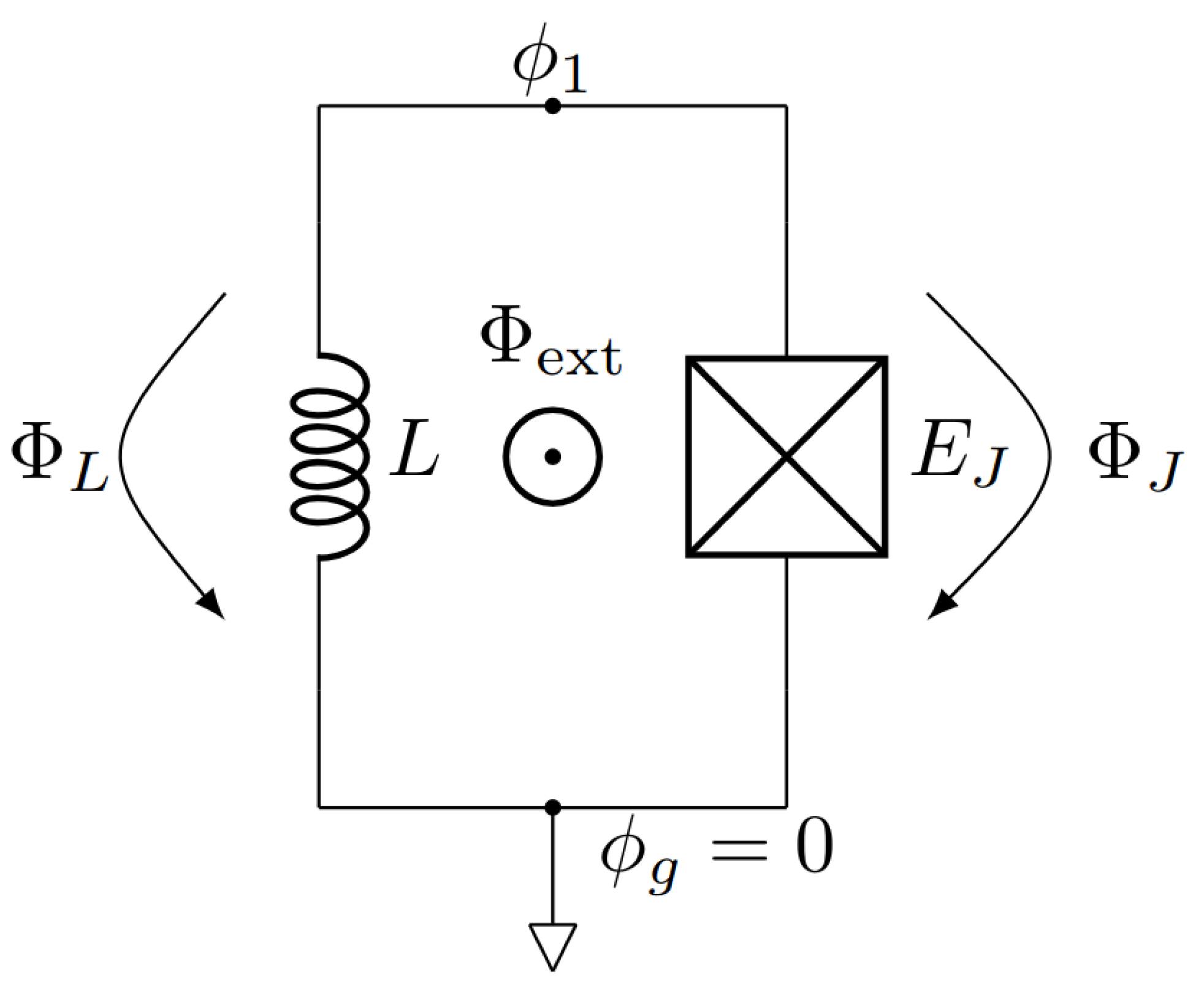
2.3. Redistributing External Fluxes

Certain terms, such as ${\varphi }_{e_i}$ (external flux terms) remain constant and do not vary with time. Since the derivative of a constant is always zero, these terms do not appear in the Hamiltonian because do not contribute to the system’s evolution and can be safely ignored in the equations of motion. More, eliminating these unnecessary terms simplifies the equations, removing complexity that does not add new information about the system.

Taking out the potential part of the system, we have:

$$\begin{array}{c}U={\varphi }_r^2{\displaystyle \frac{1}{2}}{\displaystyle \frac{L_1+L_s}{\Lambda }}+{\varphi }_1^2{\displaystyle \frac{1}{2}}({\displaystyle \frac{L_s+L_r}{\Lambda }}+{\displaystyle \frac{1}{L_2}})+{\varphi }_2^2{\displaystyle \frac{1}{2}}({\displaystyle \frac{1}{L_2}}+{\displaystyle \frac{1}{L_3}})+\cdots +{\varphi }_n^2{\displaystyle \frac{1}{2}}({\displaystyle \frac{1}{L_n}}+{\displaystyle \frac{1}{L_{n+1}}})\\ -{\varphi }_r{\varphi }_1{\displaystyle \frac{L_s}{\Lambda }}-{\varphi }_1{\varphi }_2{\displaystyle \frac{1}{L_2}}-\cdots -{\varphi }_{n-1}{\varphi }_n{\displaystyle \frac{1}{L_n}}\\ +{\varphi }_1{\varphi }_{e_1}{\displaystyle \frac{L_s+L_r}{\Lambda }}+{\varphi }_2{\varphi }_{e_2}{\displaystyle \frac{1}{L_2}}+\cdots +{\varphi }_n{\varphi }_{e_n}{\displaystyle \frac{1}{L_n}}\\ -{\varphi }_1{\varphi }_{e_2}{\displaystyle \frac{1}{L_2}}-{\varphi }_2{\varphi }_{e_3}{\displaystyle \frac{1}{L_3}}-\cdots -{\varphi }_{n-1}{\varphi }_{e_n}{\displaystyle \frac{1}{L_n}}-{\varphi }_n{\varphi }_{e_{n+1}}{\displaystyle \frac{1}{L_{n+1}}}\\ -E_{J_1}cos\left({\phi }_1\right)-E_{J_2}cos\left({\phi }_2\right)-\cdots -E_{J_n}cos\left({\phi }_n\right).\end{array}$$

(9)

By setting the potential energy U to zero and also shifting the coordinates to absorb the effect of the external flux, we solve for the stationary points, allowing us to determine how the external flux shifts the equilibrium flux values in the circuit, so setting the potential energy to zero we find the shifting due to the external flux in the system. First, we ignore the Josephson energy term and focus only on the part of the potential energy that does not include it. The potential energy matrix can be written as:

$$\mathbf{U}={\displaystyle \frac{1}{2}}{\left(\begin{array}{c}{\varphi }_r\\ {\varphi }_1\\ ⋮\\ {\varphi }_n\end{array}\right)}^{\mathbf{T}}{\displaystyle \frac{1}{\mathbf{L}}}\left(\begin{array}{c}{\varphi }_r\\ {\varphi }_1\\ ⋮\\ {\varphi }_n\end{array}\right)+{\left(\begin{array}{c}{\varphi }_r\\ {\varphi }_1\\ ⋮\\ {\varphi }_n\end{array}\right)}^{\mathbf{T}}\mathcal{A}.$$

(10)

The inductive energy term generates a quadratic potential and directly determines the flux equilibrium shift due to external flux, while the Josephson energy introduces nonlinearity that complicates the solution. If we remove the Josephson part, we are left with just the inductive part, which still gives insight into how the external flux affects the system in the absence of nonlinearity. This will be corrected when we reintroduce the Josephson part. We perform a coordinate transformation that absorbs the external flux shift and we redefine flux variables relative to this new equilibrium. Firstly, we complete the square in the potential energy expression. This mathematical technique allows us to reorganize terms, especially those involving products between flux variables and external fluxes, into a squared form that isolates the flux variables. By doing this, the external fluxes appear in a shifted form, different from their original definitions. Because the $\mathbf{1}/\mathbf{L}$ matrix is symmetric, we can write this equation, as

$$\begin{array}{c}\hfill {\mathrm{\Phi }}^T{\displaystyle \frac{1}{\mathbf{L}}}\mathbf{x}={\mathrm{\Phi }}^T\mathcal{A},\\ \hfill {\displaystyle \frac{1}{\mathbf{L}}}\mathbf{x}=\mathcal{A}.\end{array}$$

(11)

Solving this equation yields the shift vector introduced by the external fluxes, which effectively relocates their influence from the inductive terms to the Josephson junction contributions. This transformation simplifies the system by embedding the external flux effects into the Josephson phase dynamics, avoiding complications in the inductive energy terms. As a result, the flux variables are redefined to naturally incorporate external flux, leading to a more concise and intuitive formulation of the Hamiltonian. For the inductively coupled fluxonium-resonator system, solving the equation above yields the following shift vector:

$${\mathrm{x}}_{\mathrm{fluxonium}}=\left(\begin{array}{c}0\\ {\varphi }_{e_1}\end{array}\right).$$

(12)

For architectures with n Josephson junctions and $n+1$ loops, the $\mathrm{x}$ vector contains the results of the above Equation (11):

$$\mathrm{x}=\left(\begin{array}{c}-{\displaystyle \frac{L_s}{L_1+L_2+\cdots +L_n+L_{n+1}+L_s}}({\varphi }_{e_1}+{\varphi }_{e_2}+\cdots +{\varphi }_{e_n}+{\varphi }_{e_{n+1}})\\ {\displaystyle \frac{(L_2+L_3+\cdots +L_{n+1}){\varphi }_{e_1}-(L_1+L_s)({\varphi }_{e_2}+\cdots +{\varphi }_{e_{n+1}})}{L_1+L_2+\cdots +L_n+L_{n+1}+L_s}}\\ ⋮\\ {\displaystyle \frac{(L_{i+1}+\cdots +L_{n+1})({\varphi }_{e_1}+\cdots +{\varphi }_{e_i})-(L_1+\cdots +L_i+L_s)({\varphi }_{e_{i+1}}+\cdots +{\varphi }_{e_{n+1}})}{L_1+L_2+\cdots +L_n+L_{n+1}+L_s}}\\ ⋮\\ {\displaystyle \frac{(L_n+\cdots +L_{n+1})({\varphi }_{e_1}+\cdots +{\varphi }_{e_n})-(L_1+\cdots +L_{n-1}+L_s)({\varphi }_{e_n}+{\varphi }_{e_{n+1}})}{L_1+L_2+\cdots +L_n+L_{n+1}+L_s}}\\ {\displaystyle \frac{L_{n+1}({\varphi }_{e_1}+\cdots +{\varphi }_{e_n})-(L_1+\cdots +L_n+L_s){\varphi }_{e_{n+1}}}{L_1+L_2+\cdots +L_n+L_{n+1}+L_s}}\end{array}\right)=\left(\begin{array}{c}{x}_r\\ x_1\\ ⋮\\ x_i\\ ⋮\\ x_{n-1}\\ x_n\end{array}\right),$$

(13)

where i is number of the intermediate $i\mathit{th}$ loop and takes values from 1 to $(n-1)$, with n being the total number of the junctions. For two loops, we retrieve the values for the gradiometric fluxonium [27], where the effective external flux depends on the flux imbalance in the two loops, having an inductance asymmetry controlling its sensitivity to global magnetic flux variations. When the asymmetry is 0, the system achieves immunity to uniform flux noise, the spectrum being equivalent to a standard fluxonium with an equivalent flux offset:

$${\mathrm{x}}_{\mathrm{gr}.\mathrm{fluxonium}}=\left(\begin{array}{c}-{\displaystyle \frac{L_s}{L_1+L_2+L_s}}({\varphi }_{e_1}+{\varphi }_{e_2})\\ {\displaystyle \frac{L_2{\varphi }_{e_1}-(L_1+L_s){\varphi }_{e_2}}{L_1+L_2+L_s}}\end{array}\right).$$

(14)

2.4. Hamiltonian Formulation

We use the Legendre transformation $\mathcal{H}={\sum }_i{Q}_i{\dot{\varphi }}_i-\mathcal{L}$ to derive the Hamiltonian $\mathcal{H}$ from the Lagrangian $\mathcal{L}$, where $Q_i$ is the generalized charge conjugate to the flux variable ${\varphi }_i$, defined as $Q_i={\displaystyle \frac{\partial \mathcal{L}}{\partial {\dot{\varphi }}_i}}$ and ${\dot{\varphi }}_i$ is the time derivative of the node flux ${\varphi }_i$. Once the Hamiltonian is established, it acts as the system’s energy model, showing how energy is shared between the capacitors, inductors, and Josephson junctions. For this, the Hamiltonian must be quantized, transforming classical variables into quantum operators.

The quantization process involves transforming the Hamiltonian into a form where it operates on quantum states, by promoting classical variables flux and charge, into quantum operators that satisfy commutation relations. In circuit QED, qubits interact with microwave resonators in a way that allows for coherent quantum control and readout. Quantization ensures that energy transitions between discrete levels can be manipulated using microwave photons and the Hamiltonian describes the discrete set of energy levels of our system [45].

Thus, the Hamiltonian of the system is constructed based on the degrees of freedom associated with the $n+1$ loops and n Josephson junctions and the corresponding flux variables:

$$\begin{array}{c}\mathcal{H}={\displaystyle \frac{1}{2C_r}}{Q}_r^2+{\displaystyle \frac{1}{2C_1}}{Q}_1^2+\cdots +{\displaystyle \frac{1}{2C_n}}{Q}_n^2\\ +{\varphi }_r^2{\displaystyle \frac{1}{2}}{\displaystyle \frac{L_1+L_s}{\Lambda }}+{\varphi }_1^2{\displaystyle \frac{1}{2}}({\displaystyle \frac{L_s+L_r}{\Lambda }}+{\displaystyle \frac{1}{L_2}})+{\varphi }_2^2{\displaystyle \frac{1}{2}}({\displaystyle \frac{1}{L_2}}+{\displaystyle \frac{1}{L_3}})+\cdots +{\varphi }_n^2{\displaystyle \frac{1}{2}}({\displaystyle \frac{1}{L_n}}+{\displaystyle \frac{1}{L_n+1}})\\ -{\varphi }_r{\varphi }_1{\displaystyle \frac{L_s}{\Lambda }}-{\varphi }_1{\varphi }_2{\displaystyle \frac{1}{L_2}}-\cdots -{\varphi }_{n-1}{\varphi }_n{\displaystyle \frac{1}{L_n}}\\ -E_{J_1}cos({\phi }_1+x_1{\displaystyle \frac{2\pi }{{\varphi }_0}})-E_{J_2}cos({\phi }_2+x_2{\displaystyle \frac{2\pi }{{\varphi }_0}})-\cdots -E_{J_n}cos({\phi }_n+x_n{\displaystyle \frac{2\pi }{{\varphi }_0}})\end{array}$$

(15)

By setting $L_2\cdots L_{n+1}$ and ${\varphi }_{e_2}\cdots {\varphi }_{e_{n+1}}$ to zero, we recover the fluxonium limit, where the system simplifies to a single Josephson junction shunted by a large inductance [26]. This result aligns with the standard fluxonium formulation, where the inductive energy and Josephson energy define the qubit’s quantum states and the circuit behaves as an artificial atom with well defined flux dependent energy levels. Also, setting $L_3\cdots L_{n+1}$ and ${\varphi }_{e_3}\cdots {\varphi }_{e_{n+1}}$ to zero, we recover the gradiometric fluxonium limit designed to suppress sensitivity to uniform magnetic field fluctuations by incorporating a symmetric structure [27].

The new coordinates are calculated liniarizing the Lagrangian according to Smith et al. [41] and can be expressed using normal modes:

$$\begin{array}{cc}{\varphi }_r=& T_{00}{\mathrm{\Phi }}_R+T_{01}{\mathrm{\Phi }}_{Q_1}+\cdots +T_{0n}{\mathrm{\Phi }}_{Q_n}\\ {\varphi }_{q_1}=& T_{10}{\mathrm{\Phi }}_R+T_{11}{\mathrm{\Phi }}_{Q_1}+\cdots +T_{1n}{\mathrm{\Phi }}_{Q_n}\\ ⋮\\ {\varphi }_{q_n}=& T_{n0}{\mathrm{\Phi }}_R+T_{n1}{\mathrm{\Phi }}_{Q_1}+\cdots +T_{nn}{\mathrm{\Phi }}_{Q_n},\end{array}$$

(16)

where $\mathbf{T}$ is the transformation matrix (for details see Appendix B).

Introducing these expressions (16) into the Lagrangian results in a kinetic energy term that involves time derivatives of the node flux variables, specifically ${\dot{\mathrm{\Phi }}}^2$ terms, which in turn gives rise to $\ddot{\mathrm{\Phi }}$ contributions in the equations of motion. The kinetic energy term is:

$$\begin{array}{c}{T}_{kin}={\displaystyle \frac{1}{2}}(C_r{T}_{00}^2+C_{q_1}{T}_{01}^2+\cdots +C_{q_n}{T}_{0n}^2){\dot{\mathrm{\Phi }}}_R^2\\ +{\displaystyle \frac{1}{2}}(C_r{T}_{10}^2+C_{q_1}{T}_{11}^2+\cdots +C_{q_n}{T}_{1n}^2){\dot{\mathrm{\Phi }}}_{Q_1}^2\\ +\cdots +{\displaystyle \frac{1}{2}}(C_r{T}_{n0}^2+C_{q_1}{T}_{n1}^2+\cdots +C_{q_2}{T}_{nn}^2){\dot{\mathrm{\Phi }}}_{Q_n}^2\\ +(C_r{T}_{00}{T}_{01}+C_{q_1}{T}_{10}{T}_{11}+\cdots +C_{q_n}{T}_{n0}{T}_{n1}){\dot{\mathrm{\Phi }}}_R{\dot{\Phi }}_{Q_1}\\ +\cdots +(C_r{T}_{0i}{T}_{0j}+\cdots +C_p{T}_{pi}{T}_{pj}+\cdots ){\dot{\mathrm{\Phi }}}_i{\dot{\mathrm{\Phi }}}_j+\cdots ,\end{array}$$

(17)

where the cross-terms involving ${\dot{\mathrm{\Phi }}}_i{\dot{\mathrm{\Phi }}}_j$ are the mixed time derivative terms. By choosing $\mathbf{T}$ wisely, such that ${\mathbf{T}}^T\mathbf{C}\mathbf{T}=D$ (becomes diagonal), the mixed terms are eliminated, thus transforming into normal modes [46]. This ensures that the kinetic energy has no cross-terms, leaving us with n independent normal modes. This normal mode transformation redefines the variables into independent modes. By regrouping the terms in the Hamiltonian, we can identify effective parameters that characterize the system’s adjusted behavior and for the general case, the adjusted parameters are:

$$\begin{array}{cc}{\mathbf{C}}_{\mathbf{R}}& =C_r{T}_{00}^2+C_1{T}_{01}^2+\cdots +C_n{T}_{0n}^2\\ {\mathbf{C}}_{\mathbf{1}}& =C_r{T}_{10}^2+C_1{T}_{11}^2+\cdots +C_n{T}_{1n}^2\\ ⋮\\ {\mathbf{C}}_{\mathbf{n}}& =C_r{T}_{n0}^2+C_1{T}_{n1}^2+\cdots +C_n{T}_{nn}^2\end{array}$$

(18)

$$\begin{array}{c}{\mathbf{L}}_{\mathbf{R}}={\displaystyle \frac{L_1+L_s}{\Lambda }}{T}_{00}^2+\left({\displaystyle \frac{L_s+L_r}{\Lambda }}+{\displaystyle \frac{1}{L_2}}\right)T_{10}^2+\left({\displaystyle \frac{1}{L_2}}+{\displaystyle \frac{1}{L_3}}\right)T_{20}^2+\cdots +\left({\displaystyle \frac{1}{L_n}}+{\displaystyle \frac{1}{L_{n+1}}}\right)T_{n0}^2\\ -{\displaystyle \frac{L_s}{\Lambda }}{T}_{00}{T}_{10}-{\displaystyle \frac{1}{L_2}}{T}_{10}{T}_{20}-\cdots -{\displaystyle \frac{1}{L_n}}{T}_{(n-1)0}{T}_{n0}\end{array}$$

(19)

$$\begin{array}{c}{\mathbf{L}}_{\mathbf{1}}={\displaystyle \frac{L_1+L_s}{\Lambda }}{T}_{01}^2+\left({\displaystyle \frac{L_s+L_r}{\Lambda }}+{\displaystyle \frac{1}{L_2}}\right)T_{11}^2+\left({\displaystyle \frac{1}{L_2}}+{\displaystyle \frac{1}{L_3}}\right)T_{21}^2+\cdots +\left({\displaystyle \frac{1}{L_n}}+{\displaystyle \frac{1}{L_{n+1}}}\right)T_{n1}^2\\ -{\displaystyle \frac{L_s}{\Lambda }}{T}_{01}{T}_{11}-{\displaystyle \frac{1}{L_2}}{T}_{11}{T}_{21}-\cdots -{\displaystyle \frac{1}{L_n}}{T}_{(n-1)1}{T}_{n1}\\ ⋮\end{array}$$

(20)

$$\begin{array}{c}{\mathbf{L}}_{\mathbf{n}}={\displaystyle \frac{L_1+L_s}{\Lambda }}{T}_{0n}^2+\left({\displaystyle \frac{L_s+L_r}{\Lambda }}+{\displaystyle \frac{1}{L_2}}\right)T_{1n}^2+\left({\displaystyle \frac{1}{L_2}}+{\displaystyle \frac{1}{L_3}}\right)T_{2n}^2+\cdots +\left({\displaystyle \frac{1}{L_n}}+{\displaystyle \frac{1}{L_{n+1}}}\right)T_{nn}^2\\ -{\displaystyle \frac{L_s}{\Lambda }}{T}_{0n}{T}_{1n}-{\displaystyle \frac{1}{L_2}}{T}_{1n}{T}_{2n}-\cdots -{\displaystyle \frac{1}{L_n}}{T}_{(n-1)n}{T}_{nn}.\end{array}$$

(21)

After shifting the external fluxes and applying the appropriate parameter transformations, the Hamiltonian can be expressed in a form that clearly separates the harmonic dynamics of the system from its nonlinear components. Specifically, the Hamiltonian now consists of a normal mode part, which includes the capacitive and inductive energies written in terms of decoupled charge and flux variables and a Josephson junction part, which retains the nonlinearity through cosine terms dependent on the shifted phases and external fluxes. The full Hamiltonian is given by:

$$\mathcal{H}={\displaystyle \frac{1}{2}}{\mathbf{Q}}^{\mathbf{T}}{\mathbf{C}}^{-1}\mathbf{Q}+{\displaystyle \frac{1}{2}}{\mathrm{\Phi }}^{\mathbf{T}}{\displaystyle \frac{\mathbf{1}}{\mathbf{L}}}\mathrm{\Phi }+\sum _k{E}_{j_k}cos(T_k\overrightarrow{\phi }+x_k{\displaystyle \frac{2\pi }{{\mathrm{\Phi }}_0}}),$$

(22)

where $\mathbf{Q}$ is the vector containing the modified conjugate charge variables, and $\mathrm{\Phi }$ represents the vector of modified flux variables corresponding to the system’s normal modes. Additionally, $\mathbf{C}$ and ${\displaystyle \frac{\mathbf{1}}{\mathbf{L}}}$ are capacitive and inductive matrices containing the new coordinates. These flux variables are defined such that the quadratic part of the Hamiltonian becomes diagonal, effectively decoupling the modes and simplifying the analysis. Here, $T_k$ denotes the k-th row of the transformation matrix used to diagonalize the linear part of the Hamiltonian and isolate the normal modes. Additionally, $\overrightarrow{\phi }$ is the vector containing the transformed reduced flux variables, which are related to the physical phases across the Josephson junctions and appear in the nonlinear cosine terms and $x_k$ is the new equivalent external flux for the k loop. This formulation highlights the separation between the linear, diagonalizable dynamics of the system and the nonlinear contributions from the Josephson junctions. Next, to calculate the Hamiltonian matrix elements, the cosine term must be broken down using the addition formula $cos(X\pm Y)=cosXcosY\mp sinXsinY$ adapted for the number of elements in the cosine. This allows the cosine and sine matrix elements to be computed analytically through expressions involving the associated Laguerre polynomials $\mathcal{L}$, following the method outlined by Smith et al. [41].

3. Conclusions

In this work, we introduced a structured method for constructing the Hamiltonian matrix of fluxonium-based superconducting circuits, particularly for systems where the capacitance matrix is diagonal, ensuring no direct capacitive coupling between different elements of the circuit. Central to this method is a variable redefinition process that allows the complete elimination of cross-terms by selecting a set of independent variables that decouple the system through normal mode decomposition.

For the multi-loop fluxonium architecture, this redefinition has a significant outcome: all external flux contributions are fully transferred to the Josephson junction anharmonic terms. This shift simplifies the overall circuit representation and facilitates a more organized formulation of the system’s Hamiltonian. Also the matrix elements associated with the Josephson terms can be expanded using Laguerre polynomials, enabling efficient numerical diagonalization and analysis of the energy spectrum.

This approach not only aligns with known limits, such as standard fluxonium [26] and gradiometric fluxonium [27] configurations but also provides a broader framework applicable to more complex superconducting qubit circuits. By decoupling the dynamics into normal modes, we are able to isolate the behavior of each loop within the circuit. This isolation supports targeted experimental investigations, especially those involving quantum non-demolition (QND) measurements [47].

By transforming the system into a basis in which the linear part of the Hamiltonian is diagonal, the modes become decoupled at the quadratic level. This enables clearer identification of the dominant dynamical degrees of freedom and facilitates analysis of how different noise channels couple to the system.

We propose that this theoretical framework can serve as a blueprint for analyzing the dynamics of multi-loop qubits, providing the theoretical tool that helps determining the quantum dynamics of novel multi-loop superconducting circuits, which is necessary for understanding and guiding qubit characterization and control experiments. In the long run, our method provides the theoretical basis for the development of more reliable and scalable multi-loop superconducting qubit systems.

In addition to their role in quantum computing, multi-loop fluxonium-type qubits may also find applications in the emerging field of quantum interconnects. Their high impedance, enhanced coherence, and tunable nonlinear interactions make them promising candidates for mediating coherent information transfer between modular quantum systems. These features are particularly relevant in the context of long-distance entanglement distribution, quantum memory interfacing, and hybrid quantum network architectures that are central to the vision of future quantum communication systems [48].

Although our method provides a flexible theoretical framework for multi-loop superconducting circuits, its applicability is based on specific circuit characteristics. In particular, the formalism assumes a diagonal capacitance matrix and a strongly inductive network that enables mode hybridization and flux redistribution. In contrast, transmon qubits are designed to operate in the low-impedance regime, where the charging energy is small and the system’s behavior is dominated by capacitive terms. While certain elements of the approach like normal mode analysis may still be applicable, the full formalism in its current form is not directly transferable to transmon-like architectures without significant modification.

Uncertainties in parameters and imperfections during fabrication can have a noticeable impact on how well qubits perform. The modeling approach we use works especially well for studying how sensitive multi-loop circuits are to such imperfections. Because the energy terms are written directly into the Hamiltonian, changes in these values can be easily built into numerical simulations. Findings indicate that asymmetries in the inductive setup can bring back sensitivity to global flux noise and cause shifts in the circuit’s optimal operating point.

The influence of flux fluctuations and other noise sources on multi-loop fluxonium coherence properties is a critical aspect of qubit performance. While this work focuses on the theoretical formulation of the Hamiltonian, a detailed study of decoherence under realistic noise models is currently in preparation, where we use this framework to analyze how the flux, charge, quasiparticle, and critical current noise influence decoherence processes, energy level stability, and overall circuit stability.

References

1. Krantz, P.; Kjaergaard, M.; Yan, F.; Orlando, T.P.; Gustavsson, S.; Oliver, W.D. A Quantum Engineer’s Guide to Superconducting Qubits. Appl. Phys. Rev. 2019, 6, 021318. [Google Scholar] [CrossRef]
2. Kjaergaard, M.; Schwartz, M.E.; Braumüller, J.; Krantz, P.; Wang, J.I.-J.; Gustavsson, S.; Oliver, W.D. Superconducting Qubits: Current State of Play. Annu. Rev. Condens. Matter Phys. 2020, 11, 369–395. [Google Scholar] [CrossRef]
3. Huang, H.-L.; Wu, D.; Fan, D.; Zhu, X. Superconducting Quantum Computing: A Review. Sci. China Inf. Sci. 2020, 63, 180501. [Google Scholar] [CrossRef]
4. Ezratty, O. Perspective on Superconducting Qubit Quantum Computing. Eur. Phys. J. A 2023, 59, 94. [Google Scholar] [CrossRef]
5. Mamgain, A.; Khaire, S.S.; Singhal, U.; Ahmad, I.; Patel, L.A.; Helambe, K.D.; Majumder, S.; Singh, V.; Suri, B. A Review of Developments in Superconducting Quantum Processors. J. Indian Inst. Sci. 2022, 103, 633–669. [Google Scholar] [CrossRef]
6. Nguyen, L.B.; Lin, Y.-H.; Somoroff, A.; Mencia, R.; Grabon, N.; Manucharyan, V.E. High-Coherence Fluxonium Qubit. Phys. Rev. X 2019, 9, 041041. [Google Scholar] [CrossRef]
7. Siddiqi, I. Engineering High-Coherence Superconducting Qubits. Nat. Rev. Mater. 2021, 6, 875–891. [Google Scholar] [CrossRef]
8. Napoli, S.; Mercurio, A.; Lamberto, D.; Zappalà, A.; Di Stefano, O.; Savasta, S. Circuit QED Spectra in the Ultrastrong Coupling Regime: How They Differ from Cavity QED. arXiv 2024, arXiv:2408.16558. [Google Scholar] [CrossRef]
9. Zhu, G.; Ferguson, D.G.; Manucharyan, V.E.; Koch, J. Circuit QED with Fluxonium Qubits: Theory of the Dispersive Regime. Phys. Rev. B 2013, 87, 024510. [Google Scholar] [CrossRef]
10. Rocha-Aguilera, D.; Molina-Reyes, J.; Méndez-Jerónimo, G. Superconducting Qubits Based on Al Josephson Junctions and Coplanar Waveguide Resonators. In Proceedings of the 2022 IEEE International Conference on Engineering Veracruz (ICEV), Boca del Río, Mexico, 24–27 October 2022; pp. 1–6. [Google Scholar] [CrossRef]
11. Stern, M.; Kubo, Y.; Grezes, C.; Vion, D.; Esteve, D.; Bertet, P. Flux Qubits in 3D Cavities. In Research in Optical Sciences; OSA Technical Digest (Online); Optica Publishing Group: Washington, DC, USA, 2014; Paper QW1A.3. [Google Scholar] [CrossRef]
12. Rosenfeld, E.L.; Hann, C.T.; Schuster, D.I.; Matheny, M.H.; Clerk, A.A. High-Fidelity Two-Qubit Gates between Fluxonium Qubits with a Resonator Coupler. PRX Quantum 2024, 5, 040317. [Google Scholar] [CrossRef]
13. Mencia, R.A.; Lin, W.J.; Cho, H.; Vavilov, M.G.; Manucharyan, V.E. Integer Fluxonium Qubit. PRX Quantum 2024, 5, 040318. [Google Scholar] [CrossRef]
14. Rieger, D.; Günzler, S.; Spiecker, M.; Paluch, P.; Winkel, P.; Hahn, L.; Hohmann, J.K.; Bacher, A.; Wernsdorfer, W.; Pop, I.M. Granular Aluminium Nanojunction Fluxonium Qubit. Nat. Mater. 2023, 22, 1135–1141. [Google Scholar] [CrossRef] [PubMed]
15. Ding, L.; Hays, M.; Sung, Y.; Kannan, B.; An, J.; Di Paolo, A.; Karamlou, A.H.; Hazard, T.M.; Azar, K.; Kim, D.K.; et al. High-Fidelity, Frequency-Flexible Two-Qubit Fluxonium Gates with a Transmon Coupler. Phys. Rev. X 2023, 13, 031003. [Google Scholar] [CrossRef]
16. Somoroff, A.; Ficheux, Q.; Mencia, R.A.; Xiong, H.; Kuzmin, R.; Manucharyan, V.E. Millisecond Coherence in a Superconducting Qubit. Phys. Rev. Lett. 2023, 130, 267001. [Google Scholar] [CrossRef]
17. Thibodeau, M.; Kou, A.; Clark, B.K. The Floquet Fluxonium Molecule: Driving Down Dephasing in Coupled Superconducting Qubits. PRX Quantum 2024, 5, 040314. [Google Scholar] [CrossRef]
18. Ardati, W.; Léger, S.; Kumar, S.; Suresh, V.N.; Nicolas, D.; Mori, C.; D’Esposito, F.; Vakhtel, T.; Buisson, O. Using Bifluxon Tunneling to Protect the Fluxonium Qubit. Phys. Rev. X 2024, 14, 041014. [Google Scholar] [CrossRef]
19. Nesterov, K.N.; Pechenezhskiy, I.V. Measurement-Induced State Transitions in Dispersive Qubit-Readout Schemes. Phys. Rev. Appl. 2024, 22, 064038. [Google Scholar] [CrossRef]
20. Nie, K.; Bista, A.; Chow, K.; Pfaff, W.; Kou, A. Parametrically Controlled Microwave-Photonic Interface for the Fluxonium. Phys. Rev. Appl. 2024, 22, 054021. [Google Scholar] [CrossRef]
21. Lin, W.-J.; Cho, H.; Chen, Y.; Vavilov, M.G.; Wang, C.; Manucharyan, V.E. Verifying the Analogy between Transversely Coupled Spin-1/2 Systems and Inductively-Coupled Fluxoniums. New J. Phys. 2025, 27, 033012. [Google Scholar] [CrossRef]
22. Wang, T.; Wu, F.; Wang, F.; Ma, X.; Zhang, G.; Chen, J.; Deng, H.; Gao, R.; Hu, R.; Ma, L.; et al. Efficient Initialization of Fluxonium Qubits Based on Auxiliary Energy Levels. Phys. Rev. Lett. 2024, 132, 230601. [Google Scholar] [CrossRef]
23. Ma, X.; Zhang, G.; Wu, F.; Bao, F.; Chang, X.; Chen, J.; Deng, H.; Gao, R.; Gao, X.; Hu, L.; et al. Native Approach to Controlled-Z Gates in Inductively Coupled Fluxonium Qubits. Phys. Rev. Lett. 2024, 132, 060602. [Google Scholar] [CrossRef] [PubMed]
24. Hita-Pérez, M.; Jaumà, G.; Pino, M.; Garcia-Ripoll, J.J. Ultrastrong Capacitive Coupling of Flux Qubits. Phys. Rev. Appl. 2022, 17, 014028. [Google Scholar] [CrossRef]
25. Mazhorin, G.S.; Kaz’mina, A.S.; Chudakova, T.A.; Simakov, I.A.; Maleeva, N.A.; Moskalenko, I.N.; Ryazanov, V.V. Scalable Quantum Processor Based on Superconducting Fluxonium Qubits. Radiophys. Quantum Electron. 2024, 66, 893–906. [Google Scholar] [CrossRef]
26. Manucharyan, V.E.; Koch, J.; Glazman, L.I.; Devoret, M.H. Fluxonium: Single Cooper-Pair Circuit Free of Charge Offsets. Science 2009, 326, 113. [Google Scholar] [CrossRef]
27. Gusenkova, D.; Valenti, F.; Spiecker, M.; Günzler, S.; Paluch, P.; Rieger, D.; Pioraş-Ţimbolmaş, L.M.; Zârbo, L.P.; Casali, N.; Colantoni, I.; et al. Operating in a Deep Underground Facility Improves the Locking of Gradiometric Fluxonium Qubits at the Sweet Spots. Appl. Phys. Lett. 2022, 120, 054001. [Google Scholar] [CrossRef]
28. Hita-Perez, M.; Jauma, G.; Pino, M.; Garcia-Ripoll, J.J. Three-Josephson Junctions Flux Qubit Couplings. Appl. Phys. Lett. 2021, 119, 222601. [Google Scholar] [CrossRef]
29. Gusenkova, D.; Spiecker, M.; Gebauer, R.; Willsch, M.; Willsch, D.; Valenti, F.; Karcher, N.; Grünhaupt, L.; Takmakov, I.; Winkel, P.; et al. Quantum Nondemolition Dispersive Readout of a Superconducting Artificial Atom Using Large Photon Numbers. Phys. Rev. Appl. 2021, 15, 064030. [Google Scholar] [CrossRef]
30. Zhang, H.; Chakram, S.; Roy, T.; Earnest, N.; Lu, Y.; Huang, Z.; Weiss, D.K.; Koch, J.; Schuster, D.I. Universal Fast-Flux Control of a Coherent, Low-Frequency Qubit. Phys. Rev. X 2021, 11, 011010. [Google Scholar] [CrossRef]
31. Bao, F.; Deng, H.; Ding, D.; Gao, R.; Gao, X.; Huang, C.; Jiang, X.; Ku, H.S.; Li, Z.; Ma, X.; et al. Fluxonium: An Alternative Qubit Platform for High-Fidelity Operations. Phys. Rev. Lett. 2022, 129, 010502. [Google Scholar] [CrossRef]
32. Somoroff, A.; Truitt, P.; Weis, A.; Bernhardt, J.; Yohannes, D.; Walter, J.; Kalashnikov, K.; Renzullo, M.; Mencia, R.A.; Vavilov, M.G.; et al. Fluxonium Qubits in a Flip-Chip Package. Phys. Rev. Appl. 2024, 21, 024015. [Google Scholar] [CrossRef]
33. Zhang, H.; Ding, C.; Weiss, D.K.; Huang, Z.; Ma, Y.; Guinn, C.; Sussman, S.; Chitta, S.P.; Chen, D.; Houck, A.A.; et al. Tunable Inductive Coupler for High-Fidelity Gates Between Fluxonium Qubits. PRX Quantum 2024, 5, 020326. [Google Scholar] [CrossRef]
34. Schoelkopf, R.J.; Girvin, S.M. Wiring Up Quantum Systems. Nature 2008, 451, 664–669. [Google Scholar] [CrossRef] [PubMed]
35. Clarke, J.; Wilhelm, F.K. Superconducting Quantum Bits. Nature 2008, 453, 1031–1042. [Google Scholar] [CrossRef] [PubMed]
36. Girvin, S.M. Circuit QED: Superconducting Qubits Coupled to Microwave Photons. Quantum Mach. Meas. Control Eng. Quantum Syst. 2014, 96, 113–256. [Google Scholar] [CrossRef]
37. Gu, X.; Kockum, A.F.; Miranowicz, A.; Liu, Y.X.; Nori, F. Microwave Photonics with Superconducting Quantum Circuits. Phys. Rep. 2017, 718–719, 1–102. [Google Scholar] [CrossRef]
38. Devoret, M.H.; Wallraff, A.; Martinis, J.M. Superconducting Qubits: A Short Review. arXiv 2004, arXiv:cond-mat/0411174. [Google Scholar] [CrossRef]
39. You, J.Q.; Nori, F. Superconducting Circuits and Quantum Information. Phys. Today 2005, 58, 42–47. [Google Scholar] [CrossRef]
40. You, J.Q.; Nori, F. Atomic Physics and Quantum Optics Using Superconducting Circuits. Nature 2011, 474, 589–597. [Google Scholar] [CrossRef]
41. Smith, W.C.; Kou, A.; Vool, U.; Pop, I.M.; Frunzio, L.; Schoelkopf, R.J.; Devoret, M.H. Quantization of Inductively Shunted Superconducting Circuits. Phys. Rev. B 2016, 94, 144507. [Google Scholar] [CrossRef]
42. Petrescu, A.; Türeci, H.E.; Ustinov, A.V.; Pop, I.M. Fluxon-Based Quantum Simulation in Circuit QED. Phys. Rev. B 2018, 98, 174505. [Google Scholar] [CrossRef]
43. Bader, D.A.; Burkhardt, P. A Simple and Efficient Algorithm for Finding Minimum Spanning Tree Replacement Edges. J. Graph Algorithms Appl. 2022, 26, 577–588. [Google Scholar] [CrossRef]
44. García Ripoll, J.J. Quantum Information and Quantum Optics with Superconducting Circuits; Cambridge University Press: Cambridge, UK, 2022. [Google Scholar]
45. Vool, U.; Devoret, M. Introduction to Quantum Electromagnetic Circuits. Int. J. Circ. Theor. Appl. 2017, 45, 897–934. [Google Scholar] [CrossRef]
46. Rasmussen, S.E.; Christensen, K.S.; Pedersen, S.P.; Kristensen, L.B.; Bækkegaard, T.; Loft, N.J.S.; Zinner, N.T. Superconducting Circuit Companion—An Introduction with Worked Examples. PRX Quantum 2021, 2, 040204. [Google Scholar] [CrossRef]
47. Unnikrishnan, C.S. Quantum Non-Demolition Measurements: Concepts, Theory and Practice. Curr. Sci. 2015, 109, 2052–2059. Available online: https://www.jstor.org/stable/24906702 (accessed on 14 March 2023). [CrossRef]
48. Pan, J.-W.; Yin, J.; Zhang, W.; Chen, Y.-A. The Evolution of Quantum Secure Direct Communication: On the Road to the Qinternet. IEEE Commun. Surv. Tutor. 2024, 26, 1898–1949. [Google Scholar] [CrossRef]
49. Demmel, J. Applied Numerical Linear Algebra; SIAM: Philadelphia, PA, USA, 1997; Available online: https://www.stat.uchicago.edu/~lekheng/courses/302/demmel/ (accessed on 14 March 2023).
Figure 1. Schematic of a superconducting circuit based on the fluxonium architecture, comprising multiple loops. The circuit includes n Josephson junctions and n + 1 superconducting loops, each threaded by an external magnetic flux. L r and C r denote the inductance and capacitance of the resonator, respectively, while L s represents the shared inductance between the harmonic (resonator) part and the qubit part. Notably, L s constitutes a small portion of the superinductance in the first loop of the qubit section. For each loop n, L n , E J n , and ϕ ext ( n ) ϕ e n correspond to the superinductance, Josephson energy, and externally applied flux, respectively. The MST is highlighted in green, spanning the entire fluxonium-resonator architecture and serves as the foundation for selecting the branches that carry independent flux variables.
Photonics 12 00417 g001
Figure 2. Schematic of a single-loop superconducting circuit where node variables are represented by ϕ 1 and ϕ g , corresponding to the quantum phase degrees of freedom at each circuit node. Branch flux variables, denoted by Φ L and Φ J , represent the magnetic flux associated with each circuit element, such as inductors (L) and Josephson junctions ( E J ), along individual branches of the loop.
Photonics 12 00417 g002
Disclaimer/Publisher’s Note: The statements, opinions and data contained in all publications are solely those of the individual author(s) and contributor(s) and not of MDPI and/or the editor(s). MDPI and/or the editor(s) disclaim responsibility for any injury to people or property resulting from any ideas, methods, instructions or products referred to in the content.