Improving Temperature Prediction Precision for Aerial Cameras by Correcting Structure and Parameters of Thermal Network Models

Abstract

Accurate temperature prediction is a prerequisite for precise thermal control of an aerial camera, which is crucial for capturing high-resolution images. This paper introduces a methodology for improving the precision of temperature predictions generated by thermal network models for aerial cameras, which involves correcting the structure and parameters of the thermal network. The passive thermal control optimization design of the frame insulation structure and convective heat transfer coefficients ensures that key thermal parameter values are maintained within optimum ranges. Following an analysis of the change trend consistency between the predicted temperatures and the transient thermal experimental data, the thermal network structure is modified to reduce the discrepancy between the thermal network and physical models. Using the Monte Carlo algorithm, parameter spaces for key thermal parameters are explored using different sampling numbers. The optimal parameter values are then derived by satisfying the tolerance limit condition and minimizing the objective function. As the sampling number increases, the RMSE between the predicted and experimental results decreases from 1.82 °C to 1.44 °C, and the R-squared value increases from 0.78 to 0.91. The proposed correction method demonstrates its efficiency and validity in refining the accuracy of thermal network models for aerial cameras.

1. Introduction

As precision optical remote sensors, aerial cameras not only necessitate minute machining and assembly tolerances but also exhibit high sensitivity to the surrounding environment [1,2]. In the intricate and dynamic environmental conditions where aerial cameras operate, temperature fluctuation is a crucial factor that significantly affects imaging quality [3,4]. To achieve high resolution and reliability of optical systems, it is imperative to implement thermal optimization design, which heavily relies on accurate predictions of thermal characteristics obtained through thermal analysis [5,6]. The lumped-parameter thermal network (LPTN) model, which capitalizes on the analogy between heat transfer and electrical conduction mechanisms, furnishes a pragmatic and efficient approach to estimating the temperature of aerial cameras [7,8]. The LPTN model reduces the intricate problem of heat conduction to a network comprising a limited number of nodes, thereby facilitating a straightforward mathematical formulation and rapid computational speed. In the context of developing a digital twin system for an aerial camera, where prompt and precise thermal predictions are of paramount importance, the LPTN model’s computational efficiency provides a robust foundation for achieving this objective [9,10].

When establishing an LPTN model, certain simplifications and assumptions are inevitably made, potentially leading to modeling errors. Factors such as variations in processing techniques, surface properties, and the surrounding environment can lead to deviations between actual physical properties and calculated values [11,12]. It is therefore essential to update the LPTN model according to test data to guarantee more precise calculations of temperature distributions. Furthermore, the continuous refinement of the LPTN model can ensure that the digital twin system remains accurate and reliable, mirroring the real-world performance of the aerial camera.

A substantial body of research has been conducted on the subject of refining thermal network models associated with aerospace instruments. In their seminal work, Toussaint et al. [13] proposed a systematic approach to calibrating satellite thermal network models. This methodology is firmly grounded in empirical data derived from thermal balance tests. Shimoji et al. [14] enhanced pivotal parameters within the thermal network model through the application of statistical regression analysis techniques. In a successful implementation of the particle swarm optimization approach, Beck et al. [15] modified thermal model parameters with a primary emphasis on optimizing linear conductivity. Torralbo et al. [16] employed the Jacobian matrix formulation in conjunction with the Moore–Penrose pseudo-inverse method to effectively reduce the uncertainty associated with the parameters within the thermal mathematical model. Cui et al. [17] presented a thermal model updating approach that employs the Kriging model as a surrogate tool to refine the thermal design parameters of a solar spectrometer, thus obviating the necessity for repetitive finite element analysis iterations. Li et al. [18] employed a combination of Latin hypercube sampling and the coordinate rotation method to enhance the accuracy of the spacecraft’s thermal analysis model.

The Monte Carlo method, as a computational method based on probabilistic statistical theory, has also been employed to estimate the optimal values of thermal network parameters. Herrera and Sepúlveda [19] were the first to apply the Monte Carlo stochastic approximation method in satellite thermal analysis. Since then, the Monte Carlo method [20] and its variations have been the preferred methods for correcting thermal models. Cheng et al. [21] accurately adjusted the thermal model of a thermally regulated satellite during ground testing through the effective implementation of the Monte Carlo hybrid algorithm. Zhang et al. [22] refined the sensitive parameters of a miniature satellite by employing a tiered approach with the Monte Carlo mixed method. Moreover, the Monte Carlo ray tracing (MCRT) method has emerged as a potent instrument for determining the solar direct incidence area and radiation transfer coefficient, thereby bolstering the accuracy of spacecraft thermal network models, as evidenced by previous studies [23,24]. Recently, Shi et al. [25] developed an innovative predictor–corrector Monte Carlo methodology, enabling a higher degree of precision in solving thermal radiative transfer equations. On the other hand, Liu et al. [26] introduced a parameter self-correcting thermal network model, which dynamically adjusts the initial model parameters through real-time monitoring of IGBT solder layer aging. This approach effectively restores the accuracy of the thermal network model in calculating the junction temperature.

In our previous work, a lumped-parameter thermal network (LPTN) model was established for an aerial camera, and thermal control design was performed based on the model prediction. However, temperature gradients of up to 3 °C were still observed in the optical system [27]. An integrated Monte Carlo and least squares method was used in a separate study [28] to modify the key thermal parameter values, but a discrepancy of up to 4 °C remained between the calculated and measured temperatures of the lens after refinement of the thermal parameters. Later, to improve the computational accuracy of the thermal model, the genetic algorithm was used to search for global optimal parameter values to minimize the root mean square error (RMSE) between the calculated and measured temperatures to 1.07 °C [29].

In contrast to the previous work, the present study focuses on three key aspects: model structure modification, thermal parameter correction, and passive thermal control optimization design based on the thermal parameter sensitivity analysis. Parameter correction is achieved by using the Monte Carlo method as a parameter optimization algorithm. The aim is to investigate a different way to improve the accuracy of temperature projections for aerial cameras, thereby ensuring more accurate and reliable thermal control.

The remainder of this paper is as follows: Section 2 introduces the prototype of the experimental aerial camera and the original thermal network model, including the key thermal parameters and their optimum value ranges identified by thermally sensitive analysis. Section 3 presents the passive thermal control optimization design, including the optimization of the frame insulation structure and the convective heat transfer coefficients, which ensures that the values of the key thermal parameters are kept within the optimum ranges. Section 4 outlines the procedure for correcting the thermal network model. Following an analysis of the consistency between the predicted temperatures and the transient thermal experimental data, the thermal network structure is modified. The Monte Carlo algorithm is used to explore thermal parameter spaces with varying numbers of samples in order to derive optimal parameter values. A comparative analysis is performed to contrast the results of the original model with those of the updated model. Finally, concluding remarks are presented in Section 5.

2. Introduction to the Aerial Camera

2.1. Thermal Conditions of the Aerial Camera

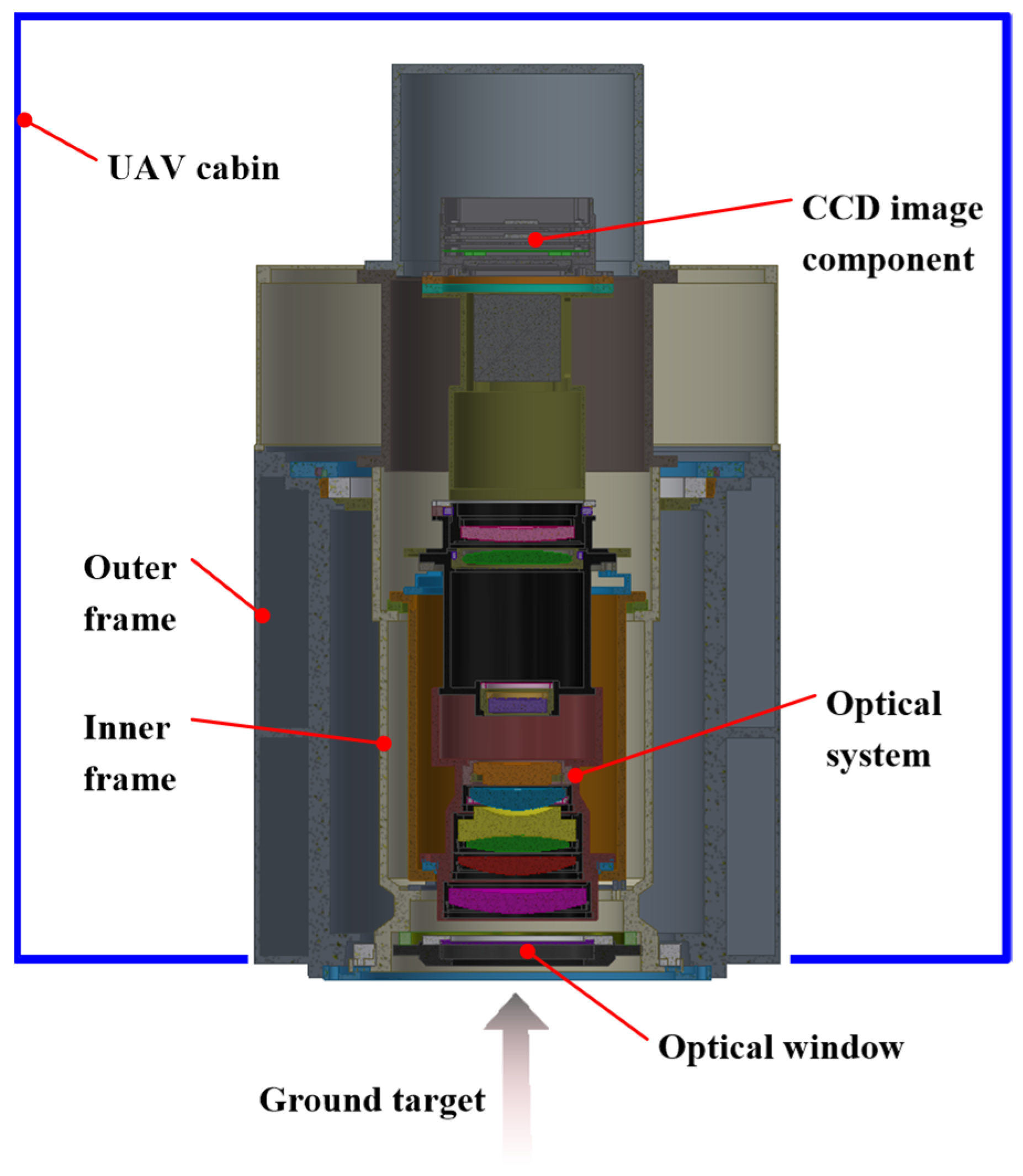
The aerial camera is mounted on an unmanned aerial vehicle (UAV), with its optical window directed vertically towards the ground target, as shown in Figure 1. The exterior surface of the optical window is in direct contact with the external environment. The thermal environment conditions and thermal control requirements are outlined in

Table 1. Thermal environment conditions and thermal control requirements.

Flight attitude	9000 m
Temperature of ambient air	−38.5 °C
Cruising speed	150 m/s
Temperature requirement of optical system	(20 ± 5) °C
Radial and axial temperature gradients	<5 °C
Thermal control power	<100 W

.

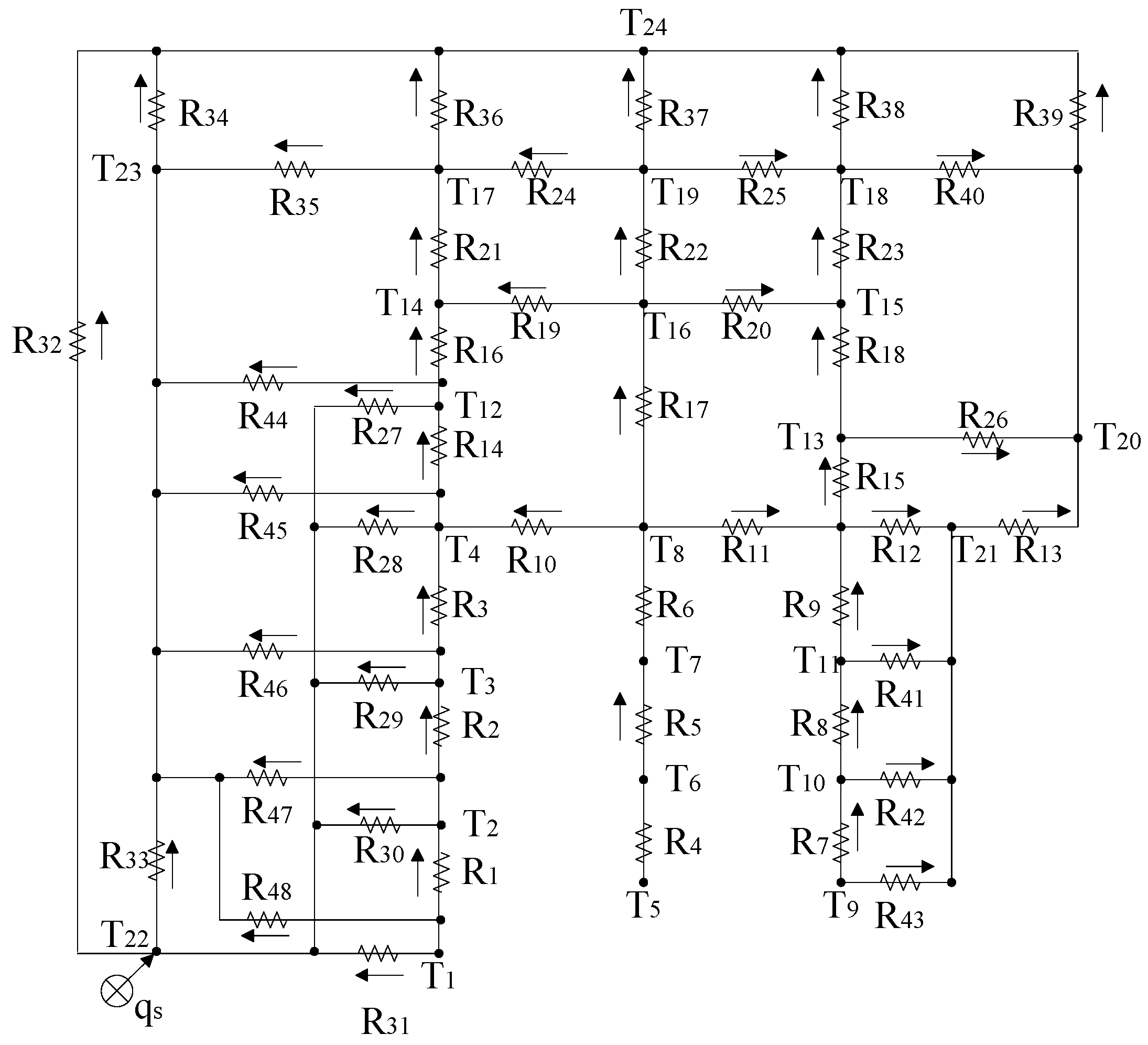
2.2. Thermal Network Model of the Aerial Camera

The physical model of the aerial camera is divided into 24 nodes. In order to simplify the thermal network model, structures such as screws, holes, and threads, which have minimal effect on the temperature, are disregarded. Components exhibiting high thermal conductivity, such as the lens barrel, inner frame, and outer frame, are sparsely divided into nodes. The lens is subject to significantly higher temperature differences in the radial direction relative to the axial direction. Consequently, the nodes of the lens are densely distributed along the radial direction. The nodes are identified based on their consolidated thermal characteristics, including temperature and heat capacity. The original thermal network of the aerial camera is structured by linking nodes through thermal resistances, representing conduction, contact, convection, or radiation, with parallel or series arrangements.

By employing Kirchhoff’s current law and Ohm’s law, the thermal balance equations for each node can be established as follows [30]:

$${(mc)}_i{\displaystyle \frac{\mathrm{d}{T}_i}{\mathrm{d}\tau }}={\displaystyle \sum _{j=1}{D}_{ij}(T_j-T_i)}+{\displaystyle \sum _j{E}_{ij}(T_j^4-T_i^4)}+{\displaystyle \sum _j{H}_{ij}(T_j-T_i)}+q_i$$

(1)

where (mc)_i is the thermal capacity; T_i and T_j are the temperature of adjacent nodes, respectively; D_ij, E_ij, and H_ij are the thermal conduction, radiation, and convection coefficients; and q_i is the total heat source of the node, including the internal heat source and external heat flow into the node.

For the heat conduction between two nodes with an interface, D_ij can be expressed as

$$D_{ij}={\displaystyle \frac{1}{\frac{L_i}{{\lambda }_i{A}_i}+\frac{1}{h_c{A}_h}+\frac{L_j}{{\lambda }_j{A}_j}}}$$

(2)

where λ_i, λ_j, L_i, L_j, and A_i, A_j are the thermal conductivity, effective thermal conductivity distance, and effective thermal conductivity area of adjacent nodes, respectively, and h_c and A_h are the contact heat transfer coefficient and contact area of adjacent nodes, respectively.

E_ij is calculated as follows:

$$E_{ij}={\displaystyle \frac{F_{ij}{A}_i\sigma }{\frac{1}{{\epsilon }_i}+\frac{1}{{\epsilon }_j}-1}}$$

(3)

where F_ij is the radiation angle coefficient between nodes i and j, σ is the Stefan–Boltzmann constant (σ = 5.67 × 10⁻⁸ W·m⁻²·K⁻⁴), and ε is the emissivity.

The expression for H_ij is

$$H_{ij}={\displaystyle \frac{1}{h_{ij}{A}_i}}$$

(4)

where h_ij is the convective heat transfer coefficient between nodes i and j, and A_i is the effective thermal conductivity area.

The total thermal resistance R_∑ of a parallel or series heat transfer between two or more nodes can be expressed as follows, respectively:

$${\displaystyle \frac{1}{R_{\sum }}}={\displaystyle \frac{1}{R_{ij}^{(1)}}}+{\displaystyle \frac{1}{R_{ij}^{(2)}}}+\cdots {\displaystyle \frac{1}{R_{ij}^{(n)}}}$$

(5)

$$R_{\sum }=R_{ij}^{(1)}+R_{ij}^{(2)}+\cdots +R_{ij}^{(n)}$$

(6)

where R_ij⁽ⁿ⁾ is the thermal resistance of the n-th heat transfer path between nodes i and j.

There are four distinct types of thermal resistance, namely R_cd, R_ct, R_cv, and R_rad. These correspond to the conductive, contact, convective, and radiation thermal resistances, respectively. The precision of temperature calculations within a thermal mathematical model is highly dependent on the accuracy of the thermal resistances utilized. The primary thermophysical parameters exerting influence on these resistances encompass the thermal conductivity of the material in question, the contact heat transfer coefficient, the external and internal convective heat transfer coefficients, and the surface emissivity.

In accordance with the findings of our preceding study [28], seven distinct categories of thermal parameters were derived from the thermal resistances. Through a thermally sensitive analysis, 11 key parameters and the optimal range of values were identified.

Table 2. Key thermal parameters of the aerial camera.

Type	Parameter	Description	Initial Value	Optimum Range
Thermal conductivity (W·m−1·°C−1)	k1	Optical components	1.0	Unadjustable
	k2	Frame	160	80–180
Convective heat transfer coefficient between two concentric cylinders (W·°C−1)	k5	Between lens barrel and inner frame	0.2	0.1–0.5
	k6	Between inner frame and outer frame	0.3	0.1–0.8
Convective heat transfer coefficient in planar cavity (W·m−2·°C−1)	k7	Between optical window and lens	7.8	2–15
	k8	Between lens barrel and rear cover	6.7	2–10
External convective heat transfer coefficient (W·m−2·°C−1)	k10	Between camera surface and environment	5	Unadjustable
Emissivity	k12	Frame surface	0.1	0.03–0.2
	k14	Optical window surface	0.4	0.2–0.9
Thermal resistance of insulation structure (°C·W−1)	k15	Frame insulation structure	50	15–50
	k16	Insulation structure of the optical window	5	3–5

illustrates the pivotal thermal parameters, together with their initial values and optimal ranges. Consequently, the correction process is exclusively applied to the values of the pivotal thermal parameters, while the initial values of the less sensitive parameters remain unaltered.

3. Passive Thermal Control Optimization Design

The findings of the sensitivity analysis of the thermal parameters have facilitated the identification of the pivotal parameters that exert a substantial influence on the temperature distribution of the optical system, in addition to their optimal value ranges. It is important to note that some of these critical parameter values are closely associated with the structural and material composition of the camera. Consequently, through the optimization of the camera’s structural design and the selection of suitable materials, it is possible to ensure that these critical parameter values remain within the optimal range, thereby facilitating the fulfillment of the temperature requirements of the aerial camera.

3.1. Optimization of the Frame Insulation Structure

As heat conduction between the lens barrel and the frame structure is the primary means by which the optical system dissipates heat to the external environment, the performance of the heat insulation structure in the aerial camera is a pivotal factor in determining the temperature distribution of the optical system. The magnitude of the thermal resistance of the structure determines the rate of heat conduction from the optical system to the external environment. It is evident that augmented thermal resistance within the heat insulation structure results in a slower decline in optical system temperature, concomitantly conserving energy resources allocated for active thermal control.

To enhance the thermal resistance, the utilization of polymer materials with low thermal conductivity is recommended for the fabrication of thermal pads. To mitigate vibrations, it is imperative that the screw material be metal; however, it should be noted that metals possess a high thermal conductivity, thereby rendering them the primary factor that limits the thermal resistance of the heat insulation structure. To address the issue of high thermal conductivity of the metal screws, the design of the heat insulation structure is optimized.

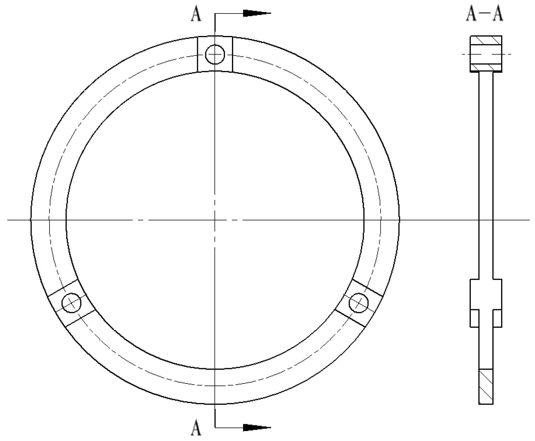
As illustrated in Figure 2, the optimized frame insulation structure consists of a heat insulation washer, a heat insulation pad, a stainless steel screw, and structural members 1 and 2. The configuration of the heat insulation pad is delineated in Figure 3, situated between structural members 1 and 2. The heat insulation washer is positioned between an annular surface of the stainless steel screw and a flat surface of structural member 1. The heat insulation washer, structural member 1, the heat insulation pad, and structural member 2 are fixedly connected by means of the stainless steel screw.

The thermal resistance of the heat insulation structure can be calculated using the following equation:

$$R={\displaystyle \frac{1}{\frac{1}{R_{c1}+\frac{L_2}{3{\lambda }_1{A}_1}+R_{c2}}+\frac{3}{R_{c3}+\frac{4L_3}{\mathsf{\pi }{\lambda }_2{D}_1^2}+R_{c4}+\frac{L_1}{{\lambda }_1{A}_2}+R_{c5}}}}$$

(7)

where R_c1, R_c2, R_c3, R_c4, and R_c5 are the contact thermal resistances between different structural elements; λ₁ and λ₂ are the thermal conductivity of the polymer material and stainless steel, respectively; L₁ and L₂ are the thickness of the insulation washer and insulation pad, respectively; L₃ is the length of the connecting section of the stainless steel screw; A₁ and A₂ are the area of the insulation pad protrusion and the bottom of the insulation washer, respectively; and D₁ and D₂ are the diameter of the stainless steel screw and the through-hole, respectively.

As demonstrated in Equation (7), it can be observed that an augmentation in L₁ and L₂, or a diminution in A₁ and A₂, can result in an escalation of thermal resistance, R. The design parameters established are L₁ = 3 mm, L₂ = 8 mm, A₁ = 54.8 mm², and A₂ = 76.4 mm². The calculated R, of 50 °C/W, falls within the optimal range of values as outlined in Table 2.

3.2. Optimization of the Convective Heat Transfer Coefficient Between Two Concentric Cylinders

The convective heat transfer coefficient between two concentric cylinders can be derived as follows:

$$h_{\mathrm{cyl}}=1.47\mathsf{\pi }L{\lambda }_f{\left[{\displaystyle \frac{g\mathrm{Pr}}{\alpha \nu {(r_m^{-3/5}+r_n^{-3/5})}^5(0.86+\mathrm{Pr})}}\right]}^{1/4}$$

(8)

where λ_f is the thermal conductivity of the fluid, L is the cylinder length, g is the gravitational acceleration, Pr is the Prandtl number, α is the thermal diffusion coefficient, ν is the kinematic viscosity, and r_m and r_n are the radius of the inner and outer cylinder, respectively.

The diameter of the lens and the spacing between the lenses are established during the optical design phase. Accordingly, the outer diameter (r_n) and length (L) of the lens barrel are fixed parameters. Consequently, the convective heat transfer coefficient between the lens barrel and inner frame can be reduced by reducing the inner diameter (r_m) of the inner frame. The dimensions of the lens barrel are specified as 70 mm in diameter and 150 mm in length, while the optimized diameter of the inner frame is designed to be 114 mm. The final inner diameter of the outer frame is thus set at 163 mm. When the air temperature fluctuates between 250 K and 300 K, the convective heat transfer coefficient between the lens barrel and the inner frame varies between 0.24 W·°C⁻¹ and 0.48 W·°C⁻¹, and the convective heat transfer coefficient between the inner and outer frames varies between 0.34 W·°C⁻¹ and 0.62 W·°C⁻¹, which aligns with the optimal range of values.

3.3. Optimization of the Convective Heat Transfer Coefficient Between the Optical Window and Lens

The convective heat transfer coefficient between the optical window and the lens can be approximated as that between two parallel planes, and the calculation method can be derived as follows:

$$h_{\mathrm{pla}}=0.27{\left({\displaystyle \frac{\mathrm{Pr}g{W}^3}{\alpha \nu (0.2+\mathrm{Pr})}}\right)}^{0.28}{\left({\displaystyle \frac{D}{W}}\right)}^{-1/4}{\displaystyle \frac{{\lambda }_f}{W}}$$

(9)

where D is the diameter of the optical window, and W is the axial distance between the optical window and the lens.

From Equation (9), it follows that h_pla is proportional to W^0.09, and the axial distance between the window and the lens can be reduced to minimize the convective heat transfer between them, provided that the structure allows for this. The diameter of the window is 40 mm, and W is designed to be 36 mm. When the average temperature of the air changes within the range of 250 K to 300 K, the convective heat transfer coefficient between the optical window and the lens changes within the range of 7.77 W·m⁻²·°C⁻¹ to 10.56 W·m⁻²·°C⁻¹, which meets the requirements of the optimal range of values.

4. Thermal Network Correction

4.1. Correction Procedure

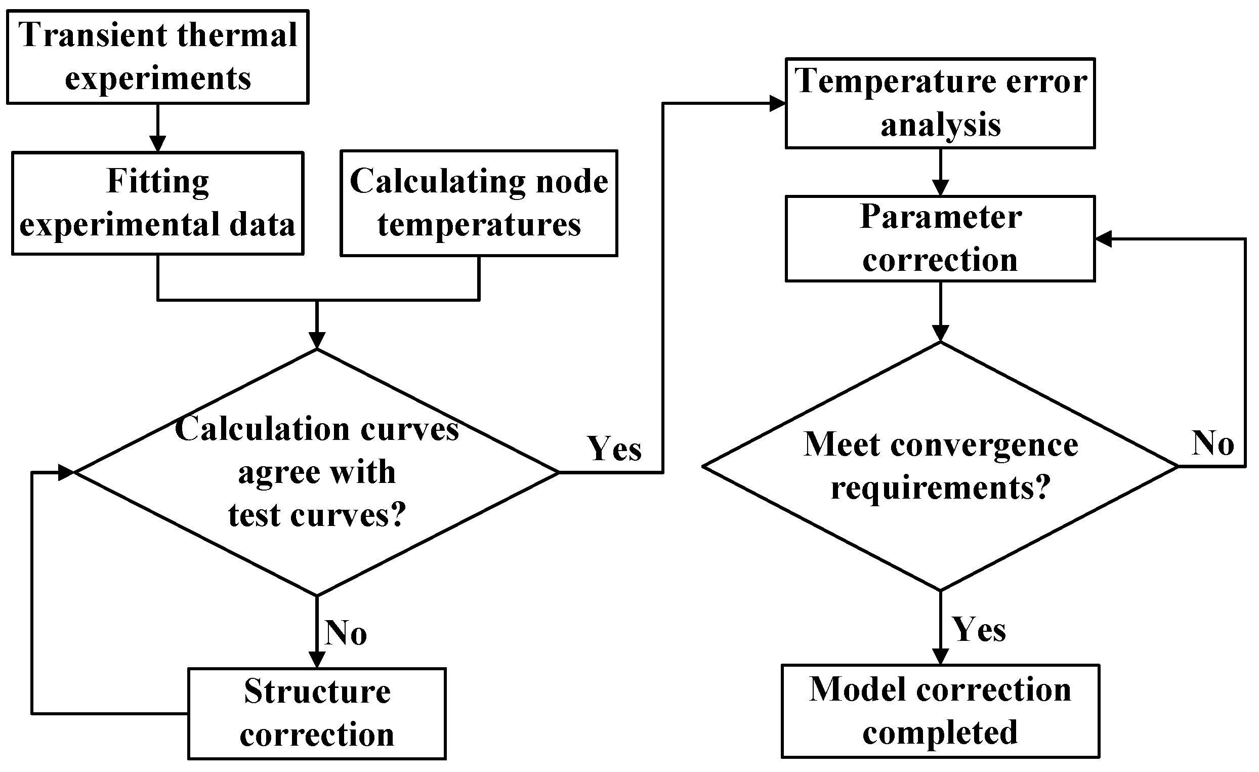
Based on the characteristics of the aerial camera thermal network model, its correction procedure has been designed and is depicted in Figure 4, providing a clear overview of the entire correction process for the thermal network model of the aerial camera.

The correction process reveals a complementary relationship between the thermal network model and the thermal experiments. Firstly, the efficacy of the thermal network model in accurately representing the characteristics of aerial cameras must be validated through a comparison of its temperature calculations with those obtained from thermal experiments. Secondly, the structure and parameters of the thermal network model must be refined using the data gained from thermal experiments. Thirdly, the reliability of the experimental data must be assessed through an error analysis of the thermal network model. It can thus be seen that both the thermal network models and the thermal experiments are indispensable, providing a solid foundation for the improvement of the thermal control design of aerial cameras and the enhancement of the reliability of thermal control systems.

In our preceding study [28], transient thermal tests of the aerial camera were conducted under 11 distinct heating conditions to obtain a more comprehensive set of experimental data, which is essential for correcting the thermal network model comprehensively. As illustrated in Figure 5, the heating films are enveloped around the lens barrel, thereby facilitating the implementation of diverse heating conditions. Temperature sensors are affixed at designated locations corresponding to each node of the thermal network model, thus enabling real-time monitoring of temperature fluctuations. Additionally, to assess the reliability of the experimental data, temperature errors attributed to the inaccuracies in the thermal parameters were studied. The results demonstrated that the measured temperature errors were within the calculated error ranges, indicating that the transient thermal test data were highly reliable and suitable for application in correcting the thermal network model.

4.2. Thermal Network Structure Correction

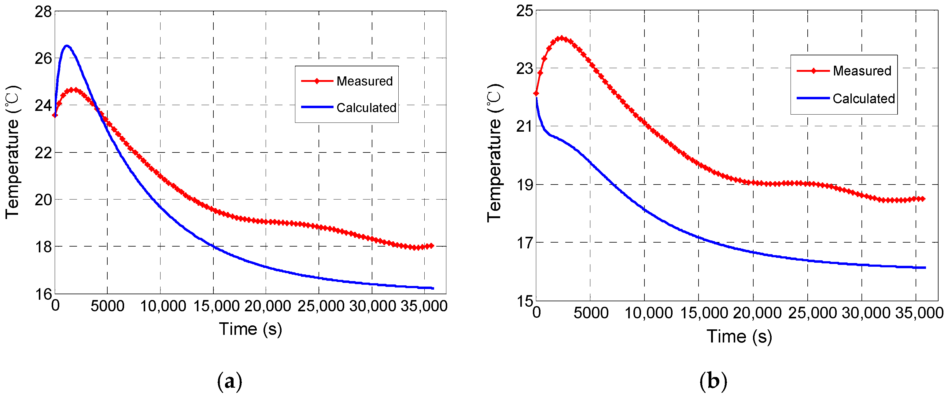
A comparative analysis of the temperature change trend at each node following the termination of the heating process reveals a discrepancy between the calculated and measured temperature curves for the window barrel. Figure 6 presents a comparison between the calculated temperature and the corresponding measured temperature. From the figure, it can be observed that the calculated temperature curve for the window and the corresponding measured temperature curve exhibit a similar trend. Both curves demonstrate a continuous rise within the first 2500 s, after which they gradually decline and reach a state of stability. In contrast, the trend of the calculated temperature curve of the window barrel and the measured temperature curve is markedly disparate. The calculated temperature declines continuously from the outset until the point of stabilization, whereas the measured temperature rises steadily from 0 to 2500 s before gradually decreasing and stabilizing.

It is evident that the positioning of the heating zone on the lens barrel results in an elevated temperature of the lens relative to that of the window component, which encompasses the window and window barrel. Subsequent to the termination of the heating process, the lens persists in the emission of heat via convection and thermal radiation, which is subsequently absorbed by the window component. Consequently, the temperature of the window component does not immediately decline, but rather continues to increase. As the heat from the lens gradually dissipates, the temperature of the lens and the window component will tend towards equilibrium. In the absence of a source of heat, the temperature of the window component will decline until it reaches the ambient temperature.

However, the modeling of the thermal network did not take into account the convection and radiation heat transfer between the window barrel and the lens. Consequently, the heat from lens 1 could not be transferred to the window barrel. This resulted in the calculated temperature continuing to decrease. It is therefore necessary to increase the convective and radiative heat transfer between the window barrel and nodes on lens 1, as well as the corresponding nodes on the lens barrel. The corrected thermal network structure is illustrated in Figure 7.

Figure 8 depicts the calculated and measured temperature curves of the window and the window barrel subsequent to the implementation of structure correction to the thermal network. It can be observed that the calculated temperature values of both the window and the window barrel are in alignment with the measured values, thereby indicating that the structure correction has been effective.

4.3. Thermal Parameter Correction

The correction of parameters in the thermal network model is an inversion problem, which involves inferring the parameter values based on the experimental temperature data of each node. The Monte Carlo algorithm is utilized to derive optimal estimates of the sensitive parameters.

The process of correcting thermal parameters using the Monte Carlo algorithm is shown in Figure 9. The specific correction procedure is delineated as follows:

(1)

The range of values for the key thermal parameters is as follows:

$$V_{\min }\le V\le V_{\max }$$

(10)

where V_min and V_max are the lower and upper limits of the key parameters, respectively, corresponding to the range of values in Table 2.

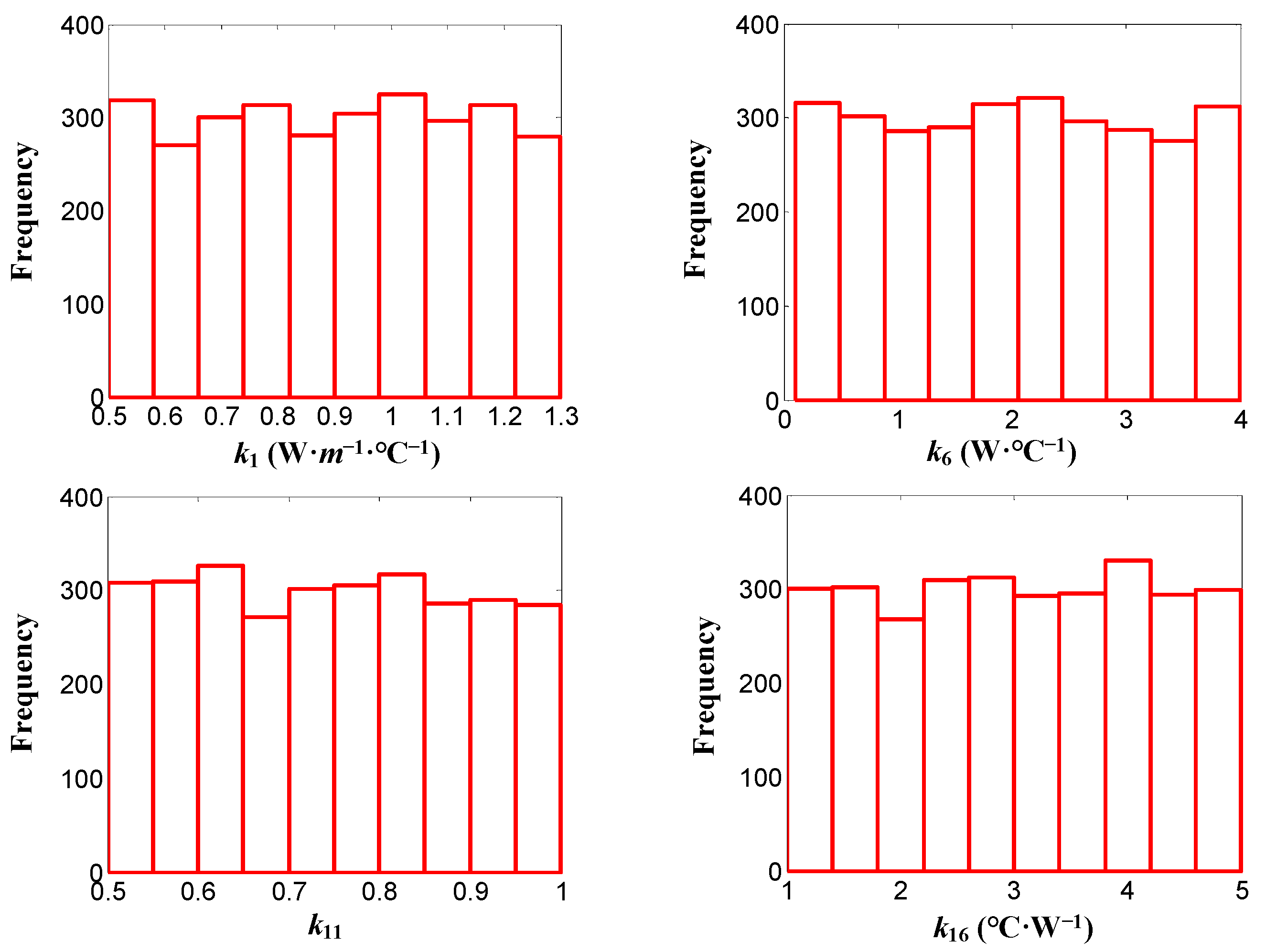
The parameter spaces for the key parameters are randomly generated, adhering to their respective ranges of values and uniform distribution patterns, with a sampling number of 3000, as depicted in Figure 10.

(2)

A set of parameter values is randomly selected from the parameter spaces and input into the thermal balance equations, as shown in Equation (1), by calculating the transient temperature variations of the nodes.

(3)

The calculated temperature curves and the measured ones are sampled at the same time interval. The calculated and measured temperature values at the sampling point are then compared on an individual basis, and the tolerance limit condition is given by

$$\left|T_i^{(u)}({\tau }_r)-T_{i\mathrm{s}}^{(u)}({\tau }_r)\right|<T_{\lim },u=1,\dots ,11$$

(11)

where T_i^(u)(τ_r) and T_is^(u)(τ_r) are the calculated and measured temperature of node i at sampling time point τ_r under the u-th heating condition, respectively, and T_lim is set as 5 °C in this case.

If the temperatures of all the sampling points satisfy Equation (11), the set of parameter values is recorded.

(4)

Repeat step (2) until all the 3000 sets of combinations of the key parameters have been validated.

(5)

Find the set of parameter values that minimize the objective function.

The objective function can be represented by the RMSE across all heating conditions between the node temperature values calculated from the combination of parameters that meet the tolerance limit condition and the measured values, which is formulated by the following equation:

$$RMS{E}_m=\sqrt{{\displaystyle \frac{{\displaystyle \sum _{v=1}^{11}{\displaystyle \sum _{i=1}^{23}{\displaystyle \sum _{r=1}^{n_u}{\left[T_i^{(m,u)}({\tau }_r)-T_{i\mathrm{s}}^{(u)}({\tau }_r)\right]}^2}}}}{23{\displaystyle \sum _{u=1}^{11}{n}_u}}}}, m=1,\cdots ,L$$

(12)

where n_u is the sampling number for calculated and measured temperature curves under the u-th heating condition, T_i^(m,u)(τ_r) is the calculated node temperature resulting from the m-th combination of parameters, and L is the total number of parameter sets that fulfill the requirements of Equation (12).

By minimizing the objective function shown in Equation (12), the optimal values of the key parameters can be determined.

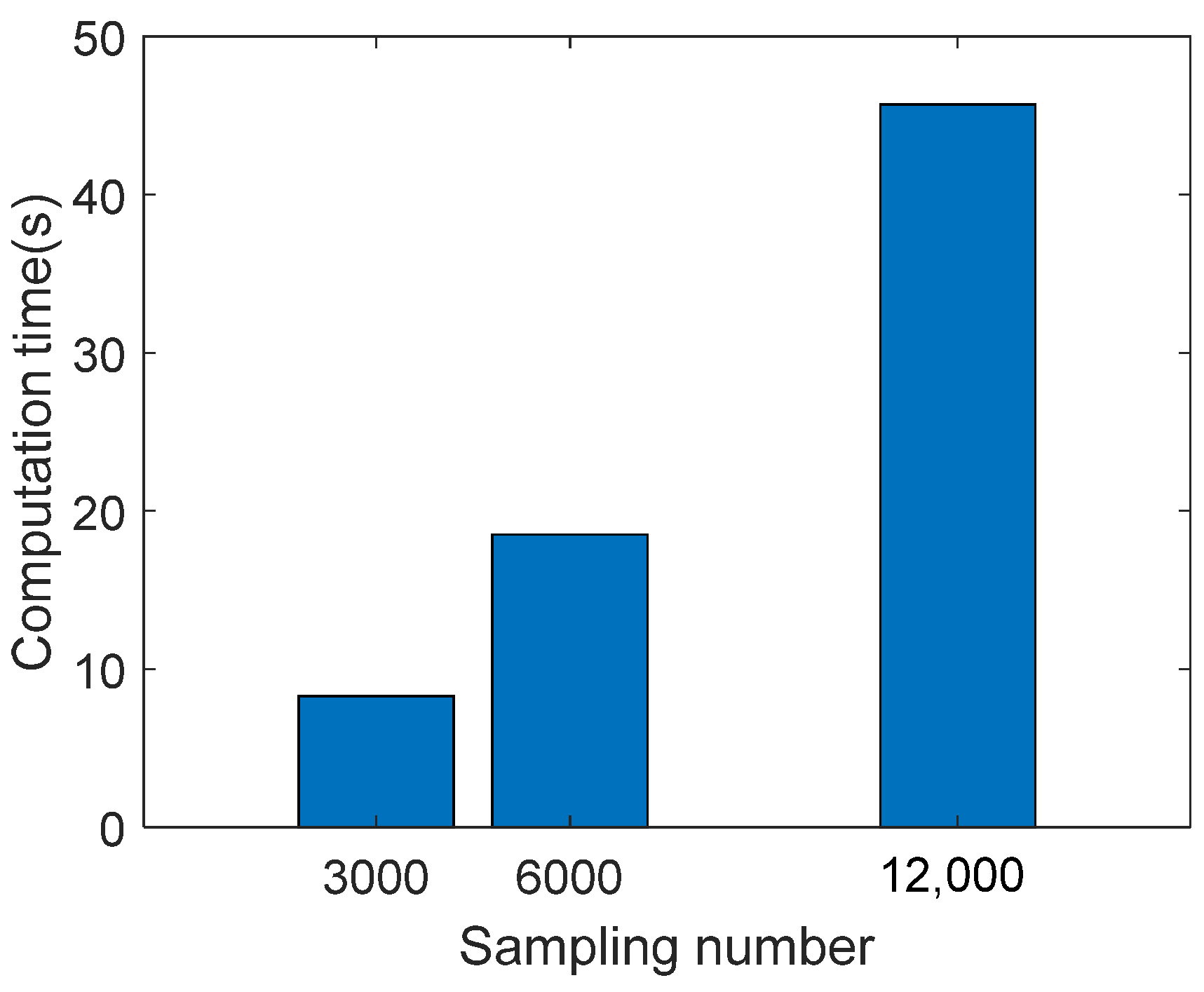
By setting the sampling number at 3000, 6000, and 12,000, respectively, it is possible to obtain the different optimal parameter combinations. It is important to note that the required computation time increases with the sampling number, as illustrated in Figure 11. However, it is important to note that as computer processor speed, memory size, and parallel computing capability improve, the computation time will reduce.

Furthermore, the predictive efficacy of the modified thermal network model can be quantified by the correlation index, R-squared:

$$R^2=1-{\displaystyle \frac{{\displaystyle \sum _{v=1}^{11}{\displaystyle \sum _{i=1}^{23}{\displaystyle \sum _{r=1}^{n_u}{\left[T_{i\mathrm{s}}^{(u)}({\tau }_r)-T_i^{(u)}({\tau }_r)\right]}^2}}}}{{\displaystyle \sum _{v=1}^{11}{\displaystyle \sum _{i=1}^{23}{\displaystyle \sum _{r=1}^{n_u}{\left[T_{i\mathrm{s}}^{(u)}({\tau }_r)-\overline{T_{i\mathrm{s}}}\right]}^2}}}}}$$

(13)

where T_i^(u)(τ_r) is the calculated node temperature resulting from the optimal parameter combination and $\overline{T_{i\mathrm{s}}}$ is the average value of the measured temperature points.

4.4. Correction Results and Discussion

To investigate the impact of varying sampling numbers on the correction outcomes, parameter spaces are constructed using sampling numbers of 3000, 6000, and 12,000, respectively, adhering to a uniform distribution.

Table 3. Minimum RMSE and R-squared along with optimal parameter values at different sampling numbers.

Sampling number	3000	6000	12,000
RMSE (°C)	1.82	1.58	1.44
R-squared	0.78	0.86	0.91
k1 (W·m−1·°C−1)	0.6	1.0	1.0
k2 (W·m−1·°C−1)	161.4	181.9	143.9
k5 (W·°C−1)	0.7	0.8	0.5
k6 (W·°C−1)	0.6	1.6	1.1
k7 (W·m−2·°C−1)	3.9	2.7	7.8
k8 (W·m−2·°C−1)	2.5	9.4	5.9
k10 (W·m−2·°C−1)	10.3	7.1	6.7
k11	0.9	0.6	1.0
k12	0.4	0.1	0.4
k14	0.7	0.4	0.4
k15 (°C·W−1)	26.1	30.0	33.2
k16 (°C·W−1)	3.9	3.0	4.6

presents the minimum RMSE values obtained, which quantify the differences between the calculated temperature values and the measured data of the nodes. Alongside the RMSE values, the associated optimal parameter values derived from these minima are provided.

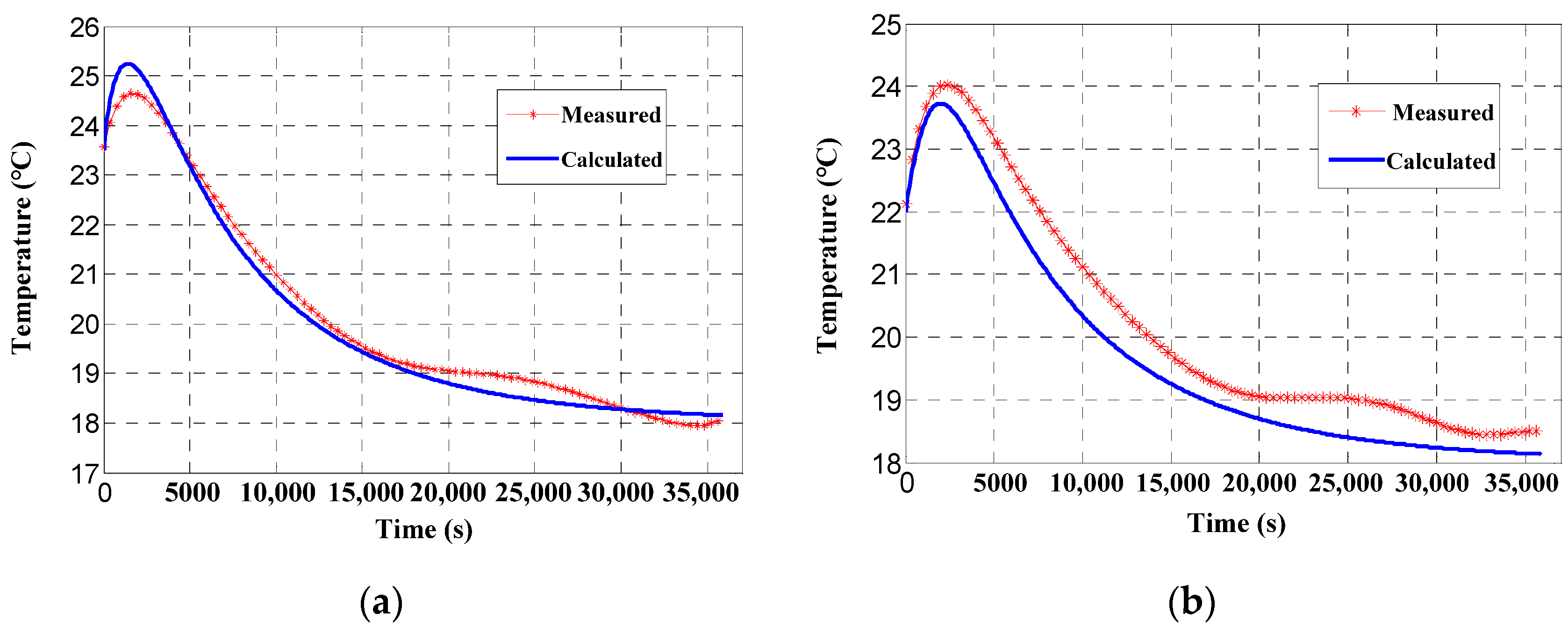
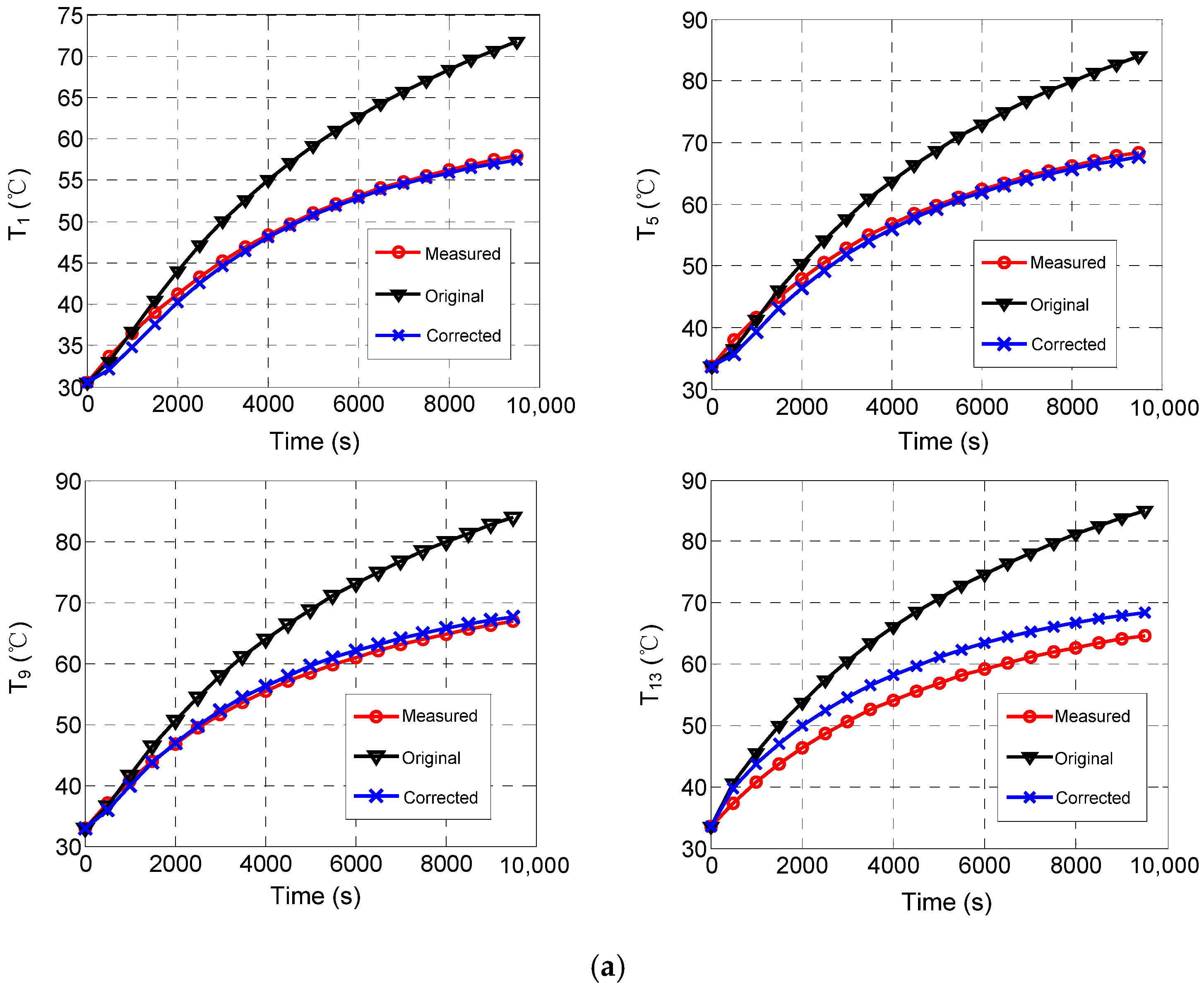
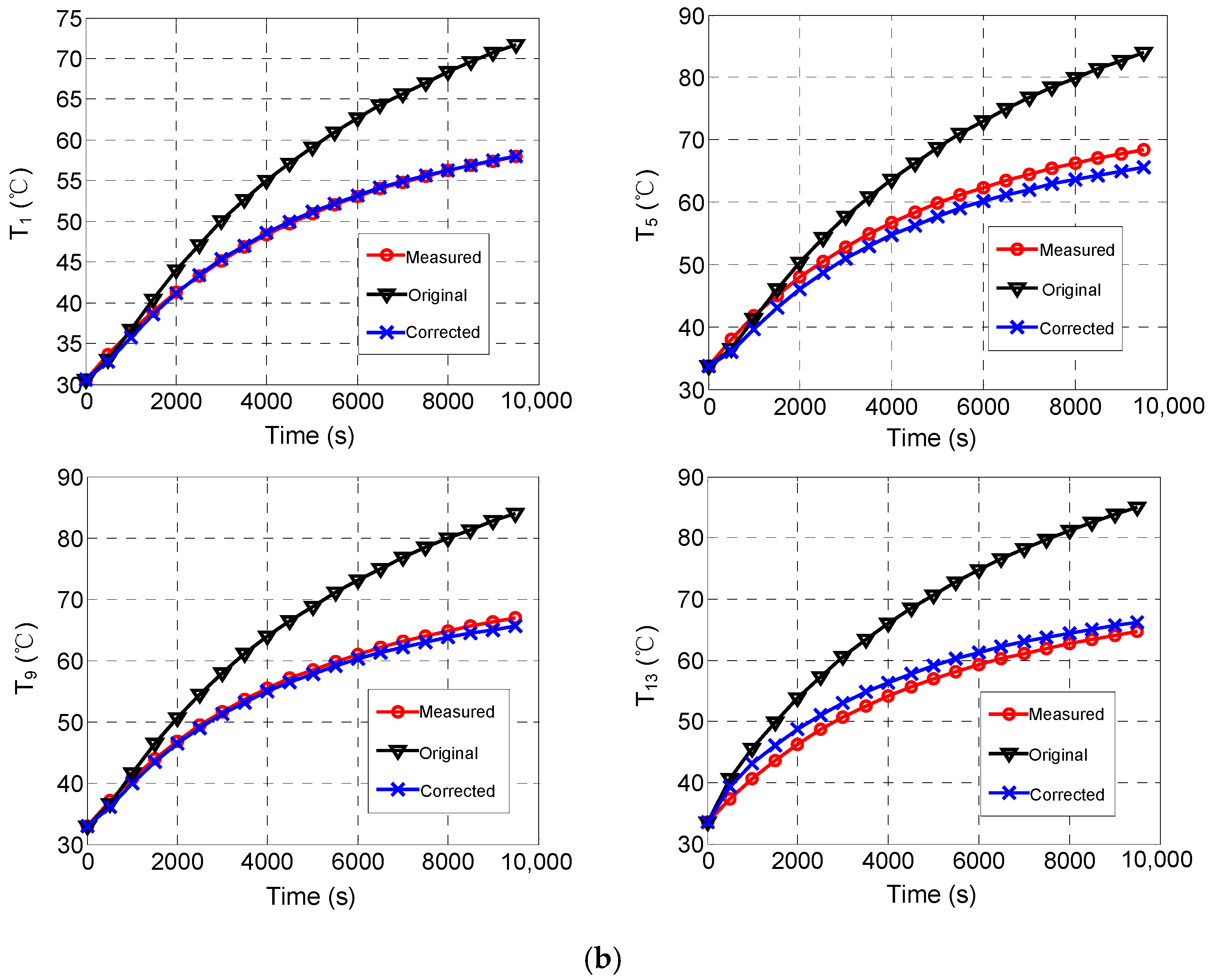
To validate the effectiveness of the parameter correction, the optimal parameter values are imported into the thermal network model for temperature calculations. As illustrated in Figure 12, the transient temperature curves for the central nodes of the lenses (nodes 1, 5, 9) and the node located on the lens barrel (node 13) are presented, with the focus being on the results obtained under heating condition 1. Prior to the implementation of the thermal parameter correction, it is evident that as the duration of the flight progresses, the temperature deviations between the calculated and measured temperatures increase significantly, with the maximum discrepancies reaching 18 °C for the lens and 22 °C for the lens barrel, respectively. Following the update of these parameters, a significant reduction in temperature deviations is observed, with the maximum relative error between the predicted and experimental results decreasing from 33.8% to 3.6%. Consequently, the calculated transient temperatures align closely with the measured data, leading to a substantial improvement in the precision of the temperature prediction capabilities of the thermal network model. The use of the modified thermal network model allows for a more accurate prediction of the temperature distribution during the flight of aerial cameras. It also promotes a deeper understanding of thermal characteristics, facilitating the development of a rational and efficient thermal control system. This in turn enables the optimization of imaging quality and the strategic allocation of thermal control resources.

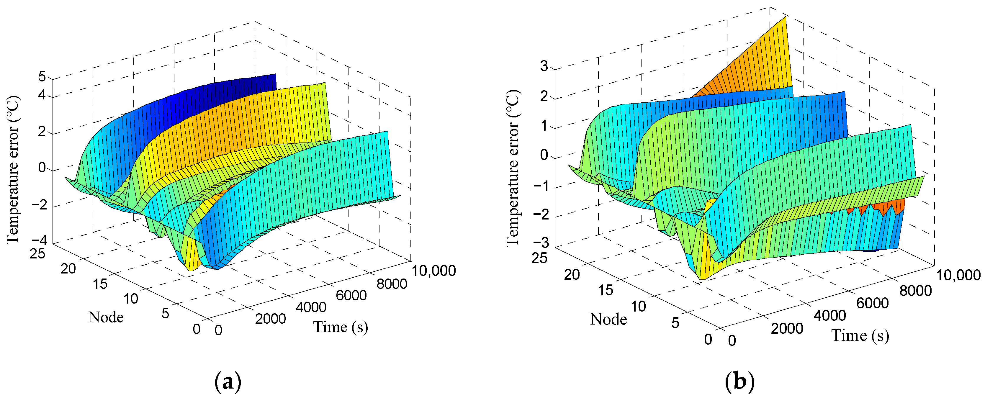
Moreover, as the number of samples within the parameter spaces increases from 3000 to 12,000, a notable decline is observed in the RMSE between the calculated and measured temperature values. In particular, the RMSE decreases from 1.82 °C to 1.44 °C, and R-squared increases from 0.78 to 0.91. This is indicative of an improvement in the precision of temperature calculations with the expansion of the sampling data. In the case of the 3000-sample correction, the calculated temperature values of the lens exhibit a high degree of correlation with the measured data, as illustrated in Figure 12a. However, the results of the lens barrel correction are unsatisfactory, with a maximum residual error of 5 °C, as illustrated in Figure 13a. However, with an increase in the number of samples to 12,000, satisfactory concordances are achieved between the calculated and measured temperature values for both the lens and the lens barrel, with a maximum residual error of 3 °C, as illustrated in Figure 13b. Moreover, 90% of the discrepancies between the calculated and measured values are within ±1.5 °C, which represents an improvement in temperature prediction accuracy compared to the results of previous studies [10,28].

5. Conclusions

This paper presents a comprehensive and systematic methodology for correcting the thermal network model, with the aim of improving the accuracy of temperature prediction and thermal performance acquisition for aerial cameras. Based on the thermally sensitive analysis results of our previous work, the passive thermal control optimization design is carried out, including the optimization of the frame insulation structure and the convective heat transfer coefficients, which ensures that the values of the key thermal parameters are kept within the optimum ranges. A comparative analysis of the temperature variation trend reveals a discrepancy between the calculated and measured temperature curves for the window barrel. Analysis of the heat transfer pathways shows that the original thermal network lacked convective and radiative heat transfer between the window barrel and the lens. After increasing the convective and radiative resistances between the window barrel and the lens, the calculated temperature values for both the window and the window barrel are in agreement with the measured values, thereby indicating the effectiveness of the structural correction. The Monte Carlo algorithm is used to explore the parameter spaces for critical parameters within their respective value ranges and uniform distribution patterns, using sampling numbers of 3000, 6000, and 12,000. The optimal parameter values are then derived by satisfying the tolerance limit condition and minimizing the objective function. As a result, the temperature predicted by the revised model shows significantly improved accuracy, with the maximum discrepancy between the predicted and experimental results reduced from 33.8% to 4.6%. Furthermore, the discrepancy between the calculated and measured temperatures decreases as the number of samples increases. This is evidenced by the reduction of the RMSE from 1.82 °C to 1.44 °C. Consequently, the precision of parameter corrections is enhanced with the expansion of the sampling data.

Compared to the previous work, the optimized thermal network model with structure and parameter correction by the Monte Carlo algorithm shows a significant improvement in the accuracy of temperature prediction. The proposed correction method provides the basis for a digital twin system of airborne cameras. In practical applications, the inability to attach sensors to the surface of optical components precludes the possibility of obtaining the online operating temperature of the optical system by direct measurement. In contrast, the digital twin system offers the potential to predict the online temperature of aerospace optical systems with a high degree of accuracy, thereby ensuring the imaging quality of the optical system through timely temperature adjustment.