Adaptive Freeform Optics Design and Multi-Objective Genetic Optimization for Energy-Efficient Automotive LED Headlights

Abstract

In addressing the design imperatives of automotive headlight miniaturization and energy conservation, this paper puts forth a design methodology for vehicle lighting systems that is predicated on free surface optics and an intelligent optimization algorithm. The establishment of the energy mapping relationship between the light source surface and the target surface is predicated on relevant performance standards. The numerical calculation is then integrated with MATLAB R2022a to obtain the free-form surface coordinate points and establish a three-dimensional model. To optimize the parameter design, a genetic algorithm is employed to fine-tune the design parameter ${\theta }_{max}$, thereby attaining the optimal ${\theta }_{max}$ that strikes a balance between volume and luminous efficiency. The experimental results demonstrate that by integrating the optimal incidence angle into the design of the high beam and low beam, the final simulation results show that the optical efficiency of the low beam is 88.89%, and the optical efficiency of the high beam is 89.40%. This enables the automotive headlamp system to achieve a balance between volume and luminous efficiency. The free-form lamp design framework proposed in this study provides a reference for the compact design and intelligent optimization of the lamp system.

1. Introduction

Amid the waves of globalization and rapid economic expansion, energy shortage and the escalating threat of environmental pollution have increasingly come to the fore as matters of grave concern [1]. China’s “14th Five-Year Plan” proposes to achieve the goal of 100% utilization of high-efficiency lighting sources, among which LED lamps as a light source of lighting have many advantages and have become one of the safe and energy-saving lighting industries with great development potential [2,3,4].

Statistical data indicate that 60% of global traffic accidents occur at night, while 22% of accidents occur in conditions of poor illumination and visibility of vehicle headlights [5,6,7]. The quality of automobile headlights for road illumination is of significant importance to drivers, as it directly affects their ability to obtain road information and subsequently their judgment of the road environment [8]. The 2022 China Semiconductor Lighting Industry Development Blue Book, published by the CSA, indicates that LED lights have become the dominant technology for automotive lighting. In addition, LED lights offer a high degree of freedom concerning external lamps, which can be utilized to great effect in automotive styling design. This enables the creation and design of a brand-new vehicle that meets the user’s personalized needs [9].

A considerable body of research has been conducted on the design of free-form mirrors for LED light sources. The design methods employed have included the grid method, the mating focal flow surface method, and the M-A method [10]. Yang et al. [11] proposed an oblique triangle energy mapping scheme and obtained a free-form reflector through geometric iterative calculation, and its headlight effect can reach 81%. Wang et al. [12] proposed a refractive design scheme for a pre-fog light lens combining an optical lens with a TIR freeform surface, and the light efficiency of the system was 76%. Zhu et al. [5] used the integrable ray mapping method to design the freeform lens of the headlamp without any other baffles or reflectors, and the energy efficiency of the optical system was more than 83.5%. Hsieh et al. [13] used a synchronous multi-surface (SMS) design method to construct a high-focus multi-surface reflector, which reduced the energy consumption of the headlight system by 70% and the optical loss by 30%. Alfred et al. [14] propose a method to use the MF concept with a combination of real and virtual light sources to achieve high-efficiency LED lighting in the automotive headlamp design. The efficiency gain was shown to improve to a significant value of 51.2% using our method while also keeping the optical design compact.

These are designed to better meet the requirements of the standard. However, little research has been performed on the initial parameters for the final mapping of optical efficiency and volume. Reverse design techniques are also emerging for automotive lamp design, but have not been widely applied due to the complexity of the algorithms and the time required to accumulate the relevant designs. In this paper, starting from the traditional light mapping method, we propose to use the control function to control the distribution of light intensity on the target surface to design the free-form surface, and to optimize the design parameters by genetic algorithms, so that the reflector can strike a balance between volume and luminous efficiency. The structure of this paper is summarized in the following section. Section 2 presents the design and evaluation of a free-form surface for the low-beam highlight, using the grid method as the design method and incorporating a control function to regulate the illuminance of the target surface. Section 3 presents the design and evaluation of the high-beam headlight. Section 4 describes a genetic algorithm used to optimize the lighting structure of the headlamp. Finally, Section 5 concludes this paper.

2. Design and Evaluation of Freeform-Based Low-Beam Headlight

2.1. Design Requirements of the Low-Beam Headlight

The national standards for low beams and high beams are identical, both of which are the requirements for the light distribution shape and brightness of the target face at 25 m from the light source. Figure 1 depicts the national standard GB25991-2010 [15] for low beam light distribution shape and illumination requirements. The overall requirements can be divided into two parts, as indicated by the center line [16], for the left side. The objective is to minimize the impact on the field of vision of oncoming drivers by preventing the generation of glare while ensuring that the illumination is as large as possible. Concerning the right side of the requirements, the illumination and the range of the largest possible are of paramount importance. The main purpose of this piece is to illuminate the road in front of the vehicle and to provide the driver with clear road information. Area I is the near lighting zone, which serves to enhance the illumination of the nearby. Area II and Area IV are high-brightness zones. These two zones occupy a central position in the driver’s field of vision. The 50V and 50R points are located in this area, which is a requirement for the illumination of the farther away places. Therefore, it is necessary to gather the light to form a high-brightness area. Region III is the anti-glare zone, comprising the left horizontal line and the right 15° line forming the dim cut-off. In this zone, the illuminance must be maintained at a very low level, with the primary objective of preventing glare from one’s headlight from affecting the driver of the oncoming vehicle [13].

2.2. LED Light Source Energy Division

The light intensity of the light emitted from the LED headlight is approximately Lambertian, and its light intensity distribution characteristics must be considered when dividing the energy of the light source. Since the ratio of the LED light-emitting aperture to the aperture of the entire optical system is greater than 1/5, the light source can be treated as a point light source, disregarding the impact of the size of the light source on the design [17]. In consideration of the LED light distribution characteristics, the division of the light source surface is typically conducted through the use of latitude and longitude lines, as illustrated in Figure 2.

Under the entire light path process, the coordinate system of light propagation is set up. Firstly, the position of the light source is set as the coordinate origin, recorded as point O. The optical axis direction points to the negative direction of the Z-axis, that is, the LED headlight is downward irradiated. The X-axis represents the direction of forward motion, while the entire light mapping trajectory for the O-point is shot in the negative direction of the Z-axis, which is the reflective surface of the collision of the reflection of the X-positive direction. This results in the formation of the target spot at X = 25,000 mm. It can be assumed that any ray of light is represented by the vector $\overrightarrow{OP}$. In this context, the angle between the vector $\overrightarrow{{OP}_{(i,j)}}$ and the negative half-axis of the X-axis is denoted by ${\theta }_i$. Furthermore, the angle denoted by ${\gamma }_j$ is the angle between the plane formed by the vector $\overrightarrow{{OP}_{(i,j)}}$ and the negative half-axis of the X-axis and the XOY plane. The combination of the angles ${\theta }_i$ and ${\gamma }_j$ forms the angle of any outgoing light source, as illustrated in Figure 3.

The LED light source is divided into M × N parts, ensuring that each part has the same luminous flux. The luminous intensity distribution $I=I_0\sin \theta \sin \gamma$ can be obtained according to the form of division. The total luminous flux emitted by the light source is:

$$\Phi ={\int }_0^{{\gamma }_{max}}d\gamma {\int }_0^{{\theta }_{max}}I\sin \theta d\theta$$

(1)

The energy of either source can be described as follows:

$$d\mathit{\Phi }={\int }_{{\gamma }_j}^{{\gamma }_{j+1}}d\gamma {\int }_{{\theta }_i}^{{\theta }_{i+1}}I\mathit{sin}\theta d\theta ={\displaystyle \frac{\mathit{\Phi }}{MN}}$$

(2)

$$d\mathit{\Phi }={\int }_{{\gamma }_j}^{{\gamma }_{j+1}}\mathit{sin}\gamma d\gamma {\int }_{{\theta }_i}^{{\theta }_{i+1}}{\mathit{sin}}^2\theta d\theta$$

(3)

Once the division is complete, the rays can be represented as vectors. For example, the ray OP(i, j) can be represented as $(-\cos \theta ,-\cos \theta \sin \gamma ,-\sin \gamma )$.

2.3. The Division of the Low Beam Target Surface

From the preceding section of the national standard for low-beam headlights, it can be observed that the principal challenges in the design of low beam free-form mirrors are the low brightness on the left side, the high brightness on the right side, and the dim cut-off line. Accordingly, the objective of this paper is to propose a novel design concept that separates the reflector into two distinct components, as illustrated in Figure 4. This approach entails dividing the reflector and the target light distribution surface from the vertical center line into two separate sections, with the reflector R1 and rectangular light distribution spot T1 situated on the left and the reflector R2 and trapezoidal light distribution spot T2 on the right.

Firstly, the left target surface, as shown in Figure 5, must be analyzed with a particular focus on the highlight area. This area will be divided into equal areas according to the gamma angle. The division line is called the control line. By controlling the distribution of points on the control line, it is possible to achieve the distribution of light spot energy on the target surface. The value of ${\gamma }_j$ in Figure 5 is equivalent to that of ${\gamma }_j$ in Figure 3. The grid is divided by the same starting point, the angle of incidence, ${\gamma }_j$, in the range of 0 to ${\gamma }_{max}$, with one side of the grid line angle divided by the control function. The length of each grid line is divided by the control function. The target surface corresponds to the ${\gamma }_j$ of the light source surface, while the target surface of the control function corresponds to the light source surface of the ${\theta }_i$.

Concerning the control line OC, it is possible to take 10 sampling points on the control line as control points. The distribution of points on the entire control line can be controlled by regulating the distribution of these 10 points, thus achieving control of the light intensity distribution. Under the established standards, the left side of the high-brightness area must be situated in the middle and lower part of the target surface to fulfill the requirements of 75L and 50L in terms of light intensity. Additionally, the center of the target surface for the 25 L also requires brightness. Consequently, it is essential to concentrate the control points in the central and lower regions to fulfill the requirements of 75L and 25L. Furthermore, the closer to the C point, the fewer the control points should be to prevent the emergence of high brightness in the I area, which does not meet the design requirements. The ratio of the distance of the control point from the origin and the length of the control line is referred to as the Proportions. The order of the control points is used to determine the curve fitting, which allows the control function of the control point to be obtained, as shown in Figure 6.

Secondly, the right side of the analysis will be divided into equal areas following the γ angle. As illustrated in Figure 7, the design specifications at this stage primarily concern the creation of a high-brightness area in the upper region and the implementation of a 45° level of dark and light cut-off lines. This is exemplified by the HV-H1-H2-H4 line, which necessitates the control line at the point to be sparse in front of the front end, before becoming dense in the middle and sparse again at the back end. This approach serves to collect the control points.

Concerning the control line MN, it is possible to take 10 sampling points on the control line as control points. The distribution of points on the control line as a whole can be controlled by regulating the distribution of these 10 points, thus achieving control of the light intensity distribution. Following the established standards, the left side of the high-brightness area must be situated in the middle and upper parts of the 75R and 50R to fulfill the requisite specifications for light intensity. Additionally, the brightness of the 25L must be maintained away from the center of the target surface. Consequently, it is essential to concentrate the control points in the upper center to achieve the appearance of the 45° cut-off line, as well as to meet the requirements of the 75L and 25L high luminance. Furthermore, the closer the control points are to the M point, the sparser they are, to avoid the appearance of high luminance in the I area, which would make it impossible to satisfy the design requirements. The control points are then collected and fitted to obtain the desired control function, as presented in Figure 8.

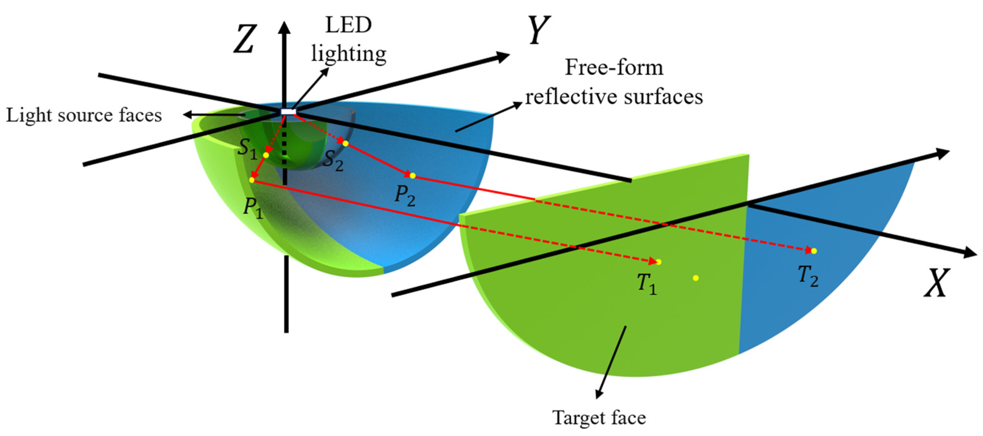
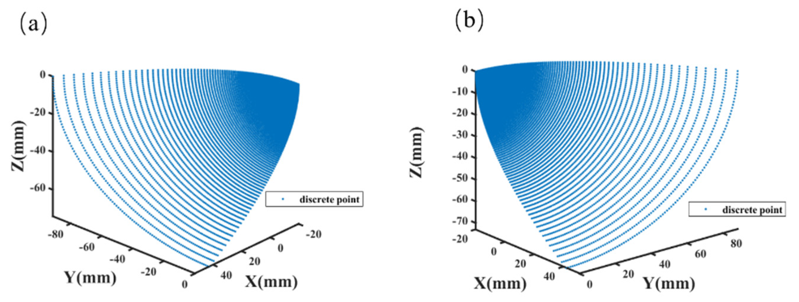
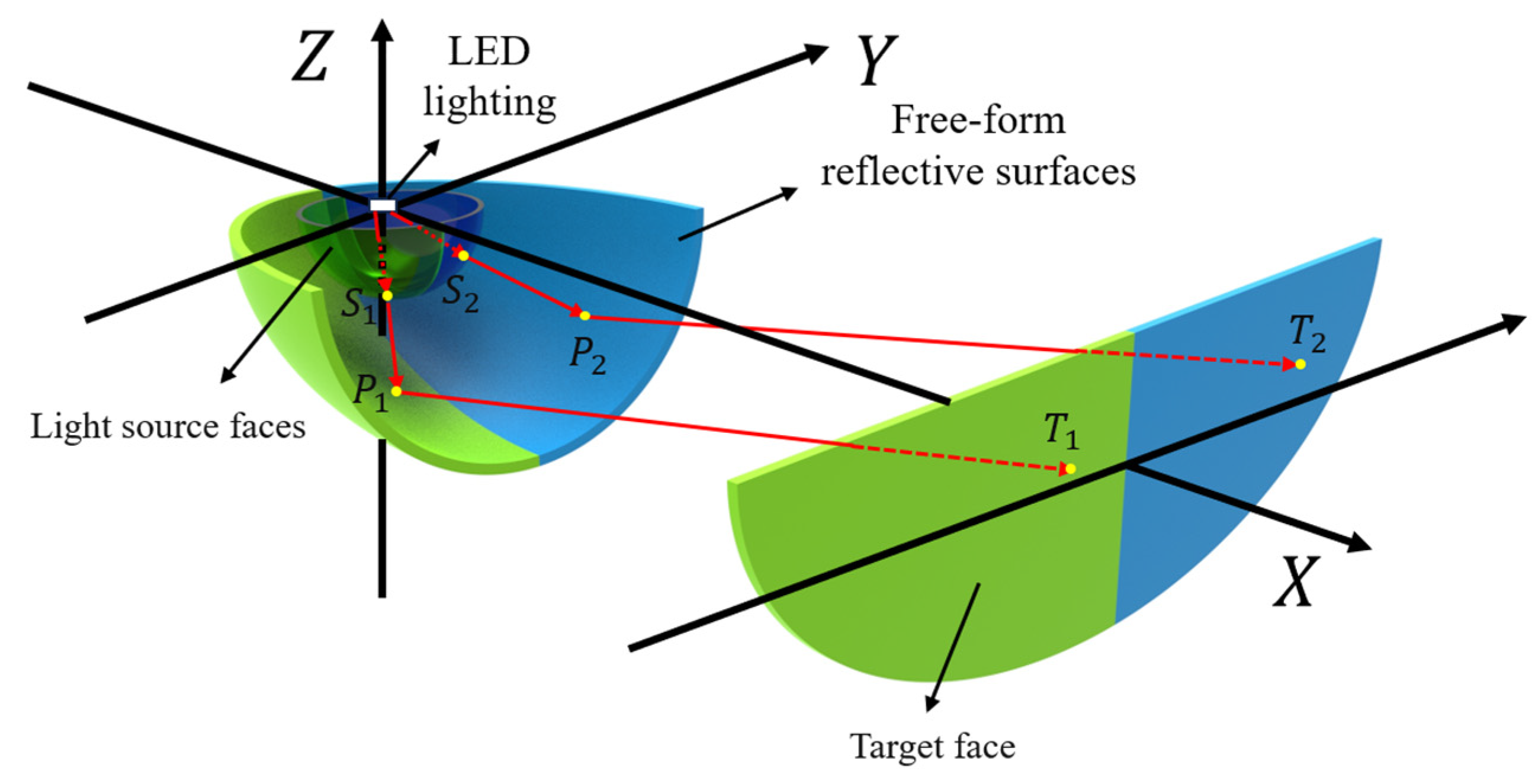
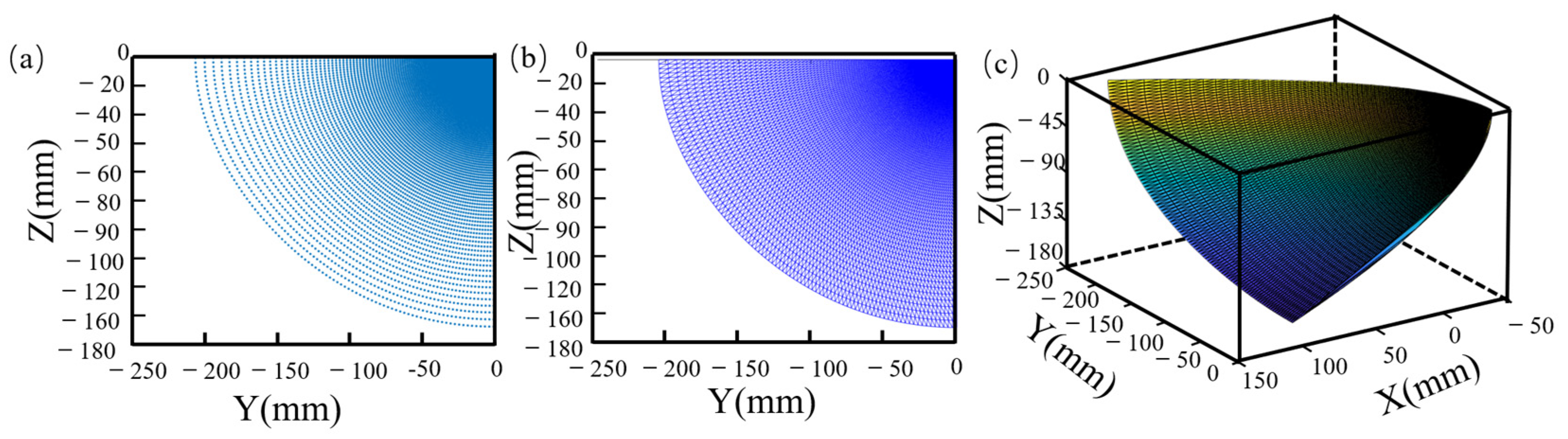
2.4. Calculation of Free-Form Surfaces for Low-Beam Headlight

In the preceding section, the light source is divided into equal energies, and the target surface is also divided into energies [18]. Finally, the light intensity distribution is determined by a control function. The mapping path for the light–mirror–target surface of the right half of the free-form reflector is shown in Figure 9. This allows for the free-form surface calculation to be carried out.

The calculation of the free-form surface is based on the modeling of the coordinates of each point on the surface. Therefore, it is necessary to obtain the positions of the points on the surface model in space before the calculation. As illustrated in Figure 10, the coordinates of each point on the free-form surface are calculated iteratively using the values of ${\theta }_i$ and ${\gamma }_j$. To illustrate, consider the calculation of one of the construction curves L₁. A certain vector of light emitted from a light source is designated as I1, and the vector of light directed to the target surface after reflection is designated as O₁.

If the light source is situated at the origin O of the three-dimensional coordinate system, and the initial point of the surface construction is P₁, the vectors $\overrightarrow{I}$ and $\overrightarrow{O}$ can be calculated based on the energy division of the light source as follows:

$$\overrightarrow{I}=\left(\sin {\theta }_i·\sin {\gamma }_j, \sin {\theta }_i·\cos {\gamma }_j, \cos {\theta }_i\right)$$

(4)

$$\overrightarrow{O}={\displaystyle \frac{\left(T_x-f\left(T_x\right),T_y-f\left(T_y\right),D-f\left(T_z\right)\right)}{\sqrt{\left({\left(T_x-f\left(T_x\right)\right)}^2+{\left(T_y-f\left(T_y\right)\right)}^2+{\left(D-f\left(T_z\right)\right)}^2\right)}}}$$

(5)

The sum of the vectors $\overrightarrow{I_1}$ and $\overrightarrow{O_1}$ can thus be calculated from the above two formulas, with the inclusion of Fresnel’s law to calculate the normal vector $\overrightarrow{N_1}$ of P₁ under the plane formed by the curve of L₁. This is as follows:

$${\left[2-2·\left(\overrightarrow{I_1}·\overrightarrow{O_1}\right)\right]}^{{\displaystyle \frac{1}{2}}}·\overrightarrow{N}=\overrightarrow{O_1}-\overrightarrow{I_1}$$

(6)

Once the normal vector, designated as $\overrightarrow{N_1}$, has been obtained at point P₁, it can be assumed that the tangent vector of $\overrightarrow{N_1}$ is $T_1$. The prolongation vector, designated as $\overrightarrow{I_2}$, intersects with the tangent vector $\overrightarrow{T_1}$ at point $P_2$, which is the next point on the curve of the free-form surface $L_1$.

$$\overrightarrow{{OP}_2}-\overrightarrow{{OP}_1}=\overrightarrow{T_1}$$

(7)

The ratio of vector $\overrightarrow{{OP}_2}$ to vector $\overrightarrow{I_2}$ is defined as x.

$$\overrightarrow{{OP}_2}=x·\overrightarrow{{ I}_2}$$

(8)

The vector–perpendicular relationship can be demonstrated by the following equation:

$$\overrightarrow{T_1}·\overrightarrow{N_1}=0$$

(9)

The solution to the three equations presented above can be determined by linking them together.

$$x={\displaystyle \frac{\overrightarrow{{OP}_1}·\overrightarrow{N_1}}{\overrightarrow{{ I}_2}·\overrightarrow{N_1}}}$$

(10)

Substitution of the x-value into the formula of $\overrightarrow{{OP}_2}$ allows the coordinates of point P2 to be determined, and this process can be repeated for all points on the L1 curve. By varying the angle of ${\gamma }_j$, the value of the subsequent construction curve can be determined, and the coordinates of all points on the free-form surface can be obtained once all construction curves have been calculated, as presented in Figure 11.

This construction method allows the entire structure curve to be derived directly from a single starting point, thus circumventing the necessity to utilize the primary curve. In the case of such surfaces in three-dimensional space, it is typically necessary to construct a primary curve and use it as an initial point to construct a secondary curve. However, this method can easily result in the accumulation of errors in the calculation, which may subsequently lead to points behind the calculation deviating more and more from the real situation. The design method presented in this paper has the potential to reduce the accumulation of errors and optimize the design efficiency.

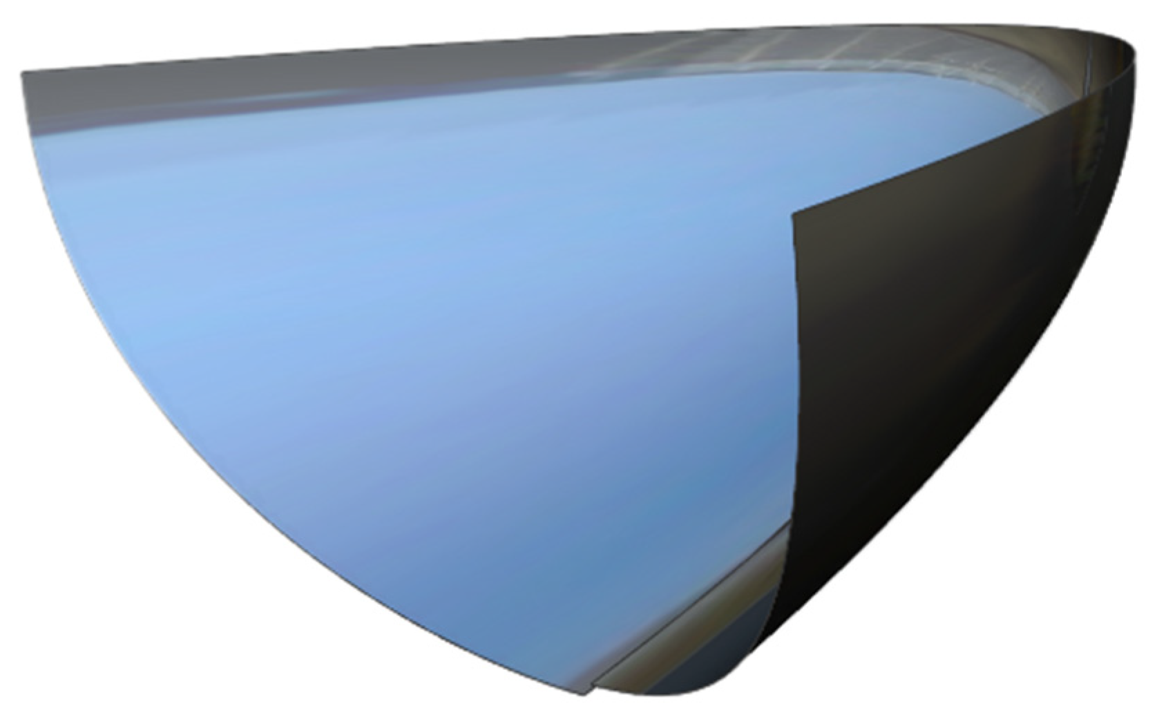
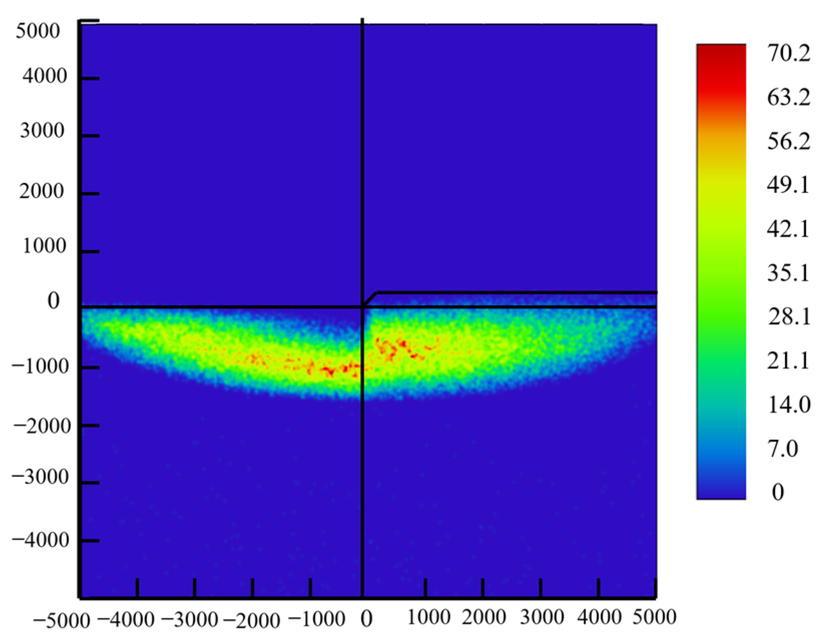
2.5. Modeling and Simulation of the Low-Beam Headlight

In the preceding section, the coordinates of the discrete points of the low beam reflector were calculated in MATLAB R2022a. Subsequently, surface fitting was performed in UG, resulting in a fitted physical model with a length of 179.08 mm, a width of 62.68 mm, and a height of 72.91 mm, as illustrated in Figure 12.

The constructed model is imported into ZEMAX 2023R2 for light tracing simulation. The light source is the same as the high beam OSRAM OSLON^® Black Flat (https://ams-osram.com/ (accessed on 16 February 2025)), with a luminous flux of 365 lm. As illustrated in Figure 13, the light source is situated at the origin, while the detector is positioned 25 m away from the origin. The simulated illuminance diagram is presented in Figure 14, while the simulated illuminance values are displayed in

Table 1. The illuminance values list of the low-beam headlight.

Test Points or Areas	Required Illuminance (lx)	Simulated Illuminance (lx)	Fulfillment of Requirements
HV	≤0.7	0.57	Yes
B50L	≤0.4	0	Yes
75R	≥12	32.16	Yes
75L	≤12	10.21	Yes
50L	≤15	13.32	Yes
50R	≥12	48.43	Yes
50V	≥6	25.71	Yes
25L	≥2	10.31	Yes
25R	≥2	7.08	Yes
III area	≤0.7	≤0.14	Yes
VI areas	≥3	≥6.85	Yes
I areas	≤2 × 50R	≤54.33	Yes

.

The simulation results indicate that the proposed design scheme is capable of meeting the design requirements and achieving superior light uniformity. In the entirety of the optical path, the light is divided into three distinct categories, as illustrated in Figure 15. These include the light that can be reflected normally, the light that is reflected twice by the reflector, and the light that is not reflected by the reflector. Among these, the light that reaches the designated area only after undergoing normal reflection is considered effective, while the remaining two categories are deemed ineffective. The energy efficiency of this optical system is calculated as follows:

$$\eta ={\displaystyle \frac{{\Phi }_T}{{\Phi }_S}}$$

(11)

The luminous flux received by the target surface, denoted by ${\Phi }_T$, and the luminous flux emitted by the light source, denoted by ${\Phi }_S$, are the two variables of interest in this context. The calculated energy utilization efficiency is 80.59%, with 19.41% of the energy dissipated throughout the process. Concerning the automobile, this component of dissipated energy can enhance the vehicles near illuminance. However, this is not a viable solution for the high beam.

The light will propagate along the X-axis in a positive direction throughout the optical system, and the reflector must remain unobscured at all times. The value of the ${\theta }_{max}$ angle has a significant impact on the optical efficiency of the system. When ${\theta }_{max}$ is small, there is a limitation on the amount of light that can be reflected to the X-axis in a positive direction. This results in a reduction in optical efficiency. Conversely, when θmax becomes larger, the mirror volume increases rapidly, which blocks the reflected light. Consequently, it is essential to strike a balance between size and optical efficiency and to assign an appropriate value to the ${\theta }_{max}$ angle. The angle ${\theta }_{max}$ is 120°. The optimization will be conducted subsequently to identify the smallest possible size with the greatest possible luminous efficiency.

3. Freeform-Based High-Beam Headlight Design and Evaluation

3.1. Design Requirements of the High-Beam Headlight

The requirements of the national standard for high beams are primarily concerned with the brightness of the light distribution screen 25 m away from the headlight and the perpendicular direction of the car driving. The standard is relatively lenient, with only five test points and intervals specified, as shown in Figure 16 and

Table 2. Light distribution requirements of the high-beam headlight.

Test Points or Areas	Required Illuminance (lx)
$E_{max}$	≥48 and ≤250
HV Point	≥$0.8 E_{max}$
1125L to HV and HV to 1125R	≥24
2250L to HV and HV to 2250R	≥6

.

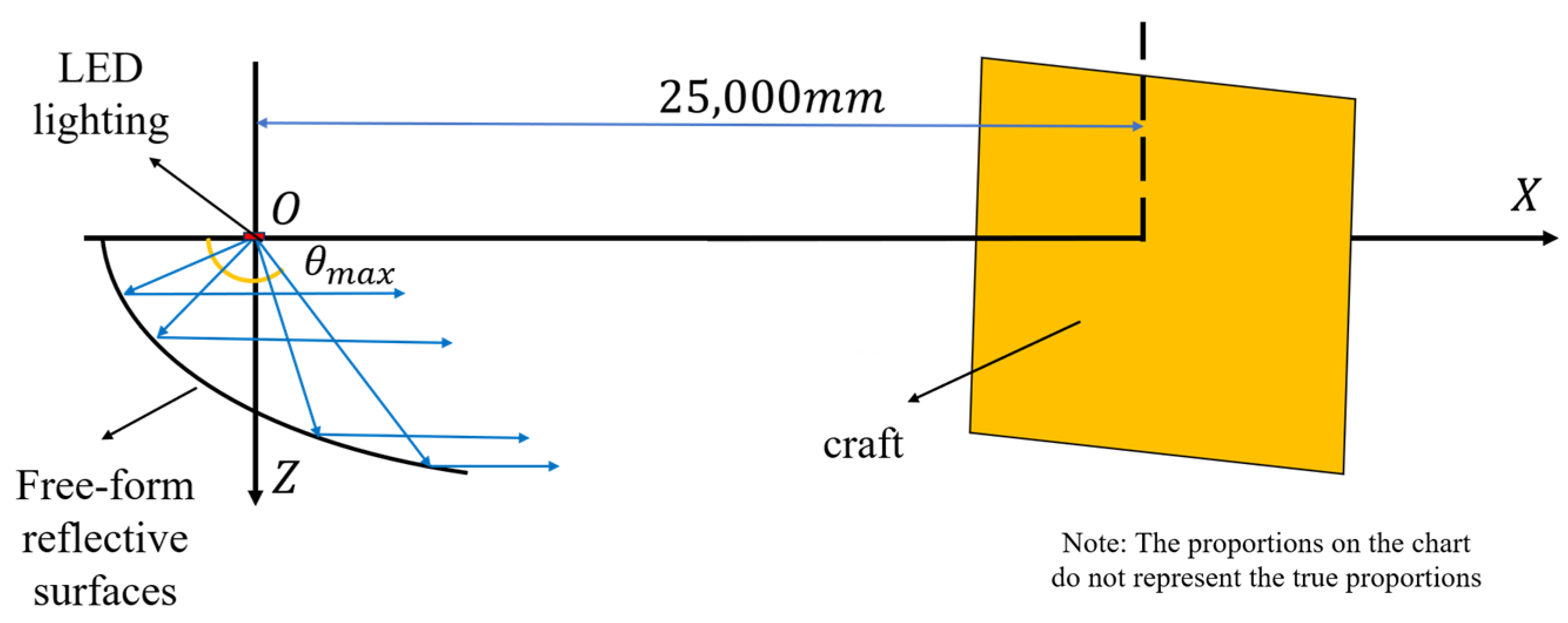
3.2. High-Beam Reflector Design

The specifications for vehicle front-illuminated high beams only require that the illuminance on the horizontal plane be met, but do not stipulate the size or shape of the light spot hitting the object surface [19]. To achieve a more reasonable distribution of light and a superior lighting effect, it is necessary to ensure that the target surface design spot division and the light source latitude and longitude of the division correspond. To align the light source division with the target surface division, it is necessary to modify the traditional target surface division. The new target surface division form is illustrated in Figure 17.

To illustrate, the control line OM may be considered a case in point. Ten sampling points on the control line may be taken as control points, and the distribution of points on the entire control line may be obtained by regulating the distribution of these ten points to achieve control of the light intensity distribution. Given that the standard design of high beam illumination is limited to the horizontal plane, it is essential to concentrate the control points in this direction. Concurrently, to achieve enhanced uniformity, it is also necessary to distribute the control points appropriately. The control points are fitted to a curve, thereby enabling the control function to be obtained, as shown in Figure 18.

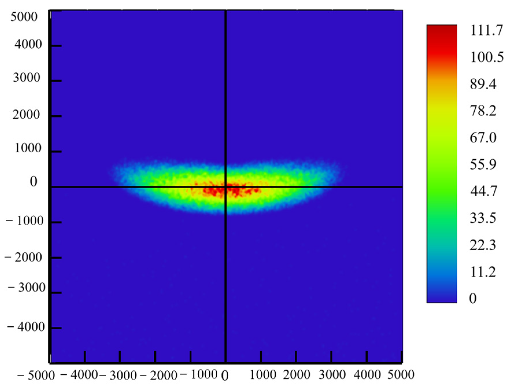
3.3. Calculation and Simulation of the Reflective Surface of High-Beam Headlight

Under the national standard for high-beam headlights, which stipulates that the target surface should be symmetric about the Z-axis, only half of the free-form mirror needs to be considered when designing the free-form mirror. Figure 19 illustrates the mapping path of the right half of the free-form mirror for high-beam headlights, which is defined by the light–mirror–target surface.

The discrete points generated by MATLAB R2022a are imported into UG for modeling purposes. The resulting free-form reflector structure of the high beam is depicted in Figure 20. The fitted physical model has a length of 157.78 mm, a width of 60.35 mm, and a height of 69.89 mm, as illustrated in Figure 20.

The generated model is employed in ZEMAX 2023R2 optical simulation software to trace the light on the designed free-form surface of the high beam. The light source is positioned at the origin, while the detector is situated 25 m away. The illuminance obtained following the simulation is presented in Figure 21.

The simulation light map indicates that the simulation results meet the GB25991-2010 requirements at each test point or area, as evidenced by the data presented in

Table 3. The results of the illuminance values list for the high-beam headlight.

Test Points or Areas	Required Illuminance (lx)	Simulated Illuminance (lx)
$E_{max}$	≥48 and ≤250	111.7
HV Point	≥$0.8 E_{max}$	97.95
1125L to HV and HV to 1125R	≥24	77.99
2250L to HV and HV to 2250R	≥6	32.11

.

The results of the simulation indicate that the $E_{max}$ value is between 48 lx and 250 lx, which is following the standard. Furthermore, the illuminance at the HV point exceeds 0.8 $E_{max}$. The lowest illuminance value from the HV point to 1125L and 1125R is 77.99 lx, which is higher than the standard requirement of 24 lx. The lowest illuminance from the HV point to 2250L and 2250R is 32 lx. The illuminance value of 11 lx is higher than the standard requirement of 6 lx. The design meets the standard requirements with a luminous efficiency of 80.69% and achieves better optical uniformity, avoiding excessive illumination in the center while improving global illumination.

4. Genetic Algorithm-Based Intelligent Optimization Method for Headlight Optical Structures

4.1. The Optimization Model Establishment

One of the most significant factors influencing the optical efficiency of the headlight reflector is the maximum angle of reflection, ${\theta }_{max}$. Increasing ${\theta }_{max}$ will result in a greater proportion of reflected light; however, this will also result in a proportion of the light that has already been reflected being blocked. Consequently, it is not possible to simply increase ${\theta }_{max}$ to improve optical efficiency. Instead, it is necessary to consider the reflector’s effect on the reflected light. Concurrently, an increase in the value of θ_max results in a rapid expansion of the reflector volume, which is contrary to the design objective of a compact configuration. Consequently, it is essential to optimize and enhance the reflector’s optical efficiency and volume simultaneously.

To illustrate this point, consider the high beam mirror. The relationship between the light effect and the volume is determined by simulating the left half of the high beam mirror. The ensuing simulation results are displayed in the accompanying Figure 22:

It is evident that an increase in volume at the initial stage results in a rapid rise in light efficiency. However, as the volume reaches 2 × 10⁵ mm, the rate of growth in light efficiency begins to decelerate. Subsequently, when the volume reaches 2 × 10⁶ mm, the growth of light efficiency becomes negligible. Consequently, the volume range between 2 × 10⁵ mm and 2 × 10⁶ mm can be considered the optimal region. Consequently, identifying the appropriate θ_max value is imperative to ascertain the optimal volume and light efficiency within the designated optimal corresponding region.

The range of ${\theta }_{max}$ can be 0° to 360°, but when ${\theta }_{max}$ ≥ π/2, the reflector will only appear to block the reflected rays; when ${\theta }_{max}$ ≥ 5π/6, the volume of the reflector becomes dramatically larger, and it does not satisfy the design requirement of a small volume. Consequently, the maximum angle of incidence, θ_max, is constrained to the range of 0° to 5π/6. Based on the value of ${\theta }_{max}$, a front-illuminated lighting system is established, and then the optical simulation is carried out in TracePro to obtain a series of data, including a simulated light map. To process the data, it is necessary to utilize an evaluation function to establish a unified index. The establishment of the simulation evaluation function must consider the impact of ${\theta }_{max}$ on optical efficiency and volume, as well as the impact of light efficiency and volume on the evaluation function of weight. This is achieved by applying the principle of normalization to establish the evaluation function.

$$f_i={\omega }_1{\displaystyle \frac{{\eta }_i-{\eta }_{min}}{{\eta }_{max}-{\eta }_{min}}}-{\omega }_2{\displaystyle \frac{V_i-V_{min}}{V_{max}-V_{min}}}$$

(12)

In the formula, the concept of normalization is employed for both $\eta$ and V. Following the normalization of these variables, the evaluation weights, ${\omega }_1$ and ${\omega }_2$, are calculated. Their size is subsequently adjusted according to the specific design requirements. Finally, the system is optimized to identify the value of ${\theta }_{max}$ in the case of the maximum value of $f_i$.

The optimization of free-form surfaces is a subcategory of optimal path optimization. Several optimal path algorithms can be applied in the optimization process of the design of the front-illuminated lighting science system, including the genetic algorithm, annealing algorithm, and particle swarm algorithm [20]. In the optimization process of this system, it is necessary to perform direct operations on the free surface. There is no qualification of derivation or function continuity, which makes it impossible to obtain a definitive rule to guide the search space of optimization. After comprehensive consideration, the genetic algorithm was selected as the optimal method for optimization [21]. This approach allows us to identify the optimal solution without having to determine the optimal result, as the nature of the optimization process is not always clear. Instead, we focus on eliminating suboptimal solutions and iterating until we reach the optimal solution without easily falling into a local optimum. Consequently, genetic algorithms are an optimal choice for optimizing free-form surfaces, as they facilitate the identification of the optimal ${\theta }_{max}$ that balances light efficiency and volume [22].

4.2. Optimization Process for Headlight Optical Structures

The previously mentioned design method for the free-form reflector for the low and high-beam headlights was employed to generate a point cloud in MATLAB R2022a. The boundaries of the point cloud are identified to ascertain the extent of the space occupied by the mirror, thereby enabling the calculation of its volume. Concurrently, to iterate the genetic algorithm, it is necessary to automate the modeling process. This involves selecting the point cloud to be processed in MATLAB R2022a, after which the points are processed to create an STL solid file.

The point cloud data obtained in the previous section were initially reduced to a two-dimensional state to obtain the projection of the point cloud image onto the YZ coordinate plane, as shown in Figure 23a. The points projected into the YZ surface are then processed using the Delaunay algorithm [23] to obtain a triangulation connection list of the point cloud within the YZ projection plane, as shown in Figure 23b. This list contains information on the number of triangulation surfaces formed by the dissections of this point cloud and the points corresponding to the vertices of each triangulation surface. The 2D triangulation connection list for the mirror-free form surface is identical to that of the 3D case, thus enabling mapping to the 3D case. The triangulated connections are mapped to the coordinates of their associated vertices in three dimensions, as presented in Figure 23c, and the triangulated connections are then written to a binary STL file with the coordinates of the vertices. This concludes the CAD modeling process, which was conducted using MATLAB to process the point cloud data.

The STL solid model is constructed and then the ZEMAX kernel is invoked with MATLAB to simulate the system using a sequence-free model. The relevant parameters of the LED light source were set at a distance of 25,000 mm from the light source in the location of the rectangular detector, which was 10,000 mm long and 8000 mm wide. This detector was imported into the established STL solid file and given the material data of the reflector. The ray tracing was then executed to complete the simulation process. Finally, the collected pixel information of the detector was used to derive the optical efficiency using MATLAB R2022a. The collected pixel information from the detector is used to derive the optical efficiency.

To optimize the optical efficiency and volume of the free-form surface, the genotype ${\theta }_{max}$ is employed as the screening criterion, with the free-form surface individual under this genotype being obtained through iterative computation and MATLAB modeling. The evaluation function, calculated following the normalization of volume and light efficiency, serves as the fitness function in the genetic algorithm, enabling the determination of the fitness of the individual. A roulette algorithm was employed to identify free-form individuals with low light efficiency. It is still possible to select surfaces with low fitness using roulette, although the probability of this occurring is low and the genes are not completely discarded. Consequently, the most exemplary members of the preceding population are combined with a certain probability of forming a new population through a selection operation, which results in the reproduction of offspring [24].

$$P_i={\displaystyle \frac{f_i}{\sum _{k=1}^M{f}_k}}$$

(13)

Accordingly, the optimal individuals from the previous generation are combined with a certain probability of forming a new generation, to achieve the reproduction of offspring.

As the genetic algorithm iterates to identify the optimal value, the iteration process cannot be expressed as a function. Consequently, the value of the iteration process is not clear. The termination of the evolutionary conditions is indicated by the termination of the genetic generation, as shown in Figure 24.

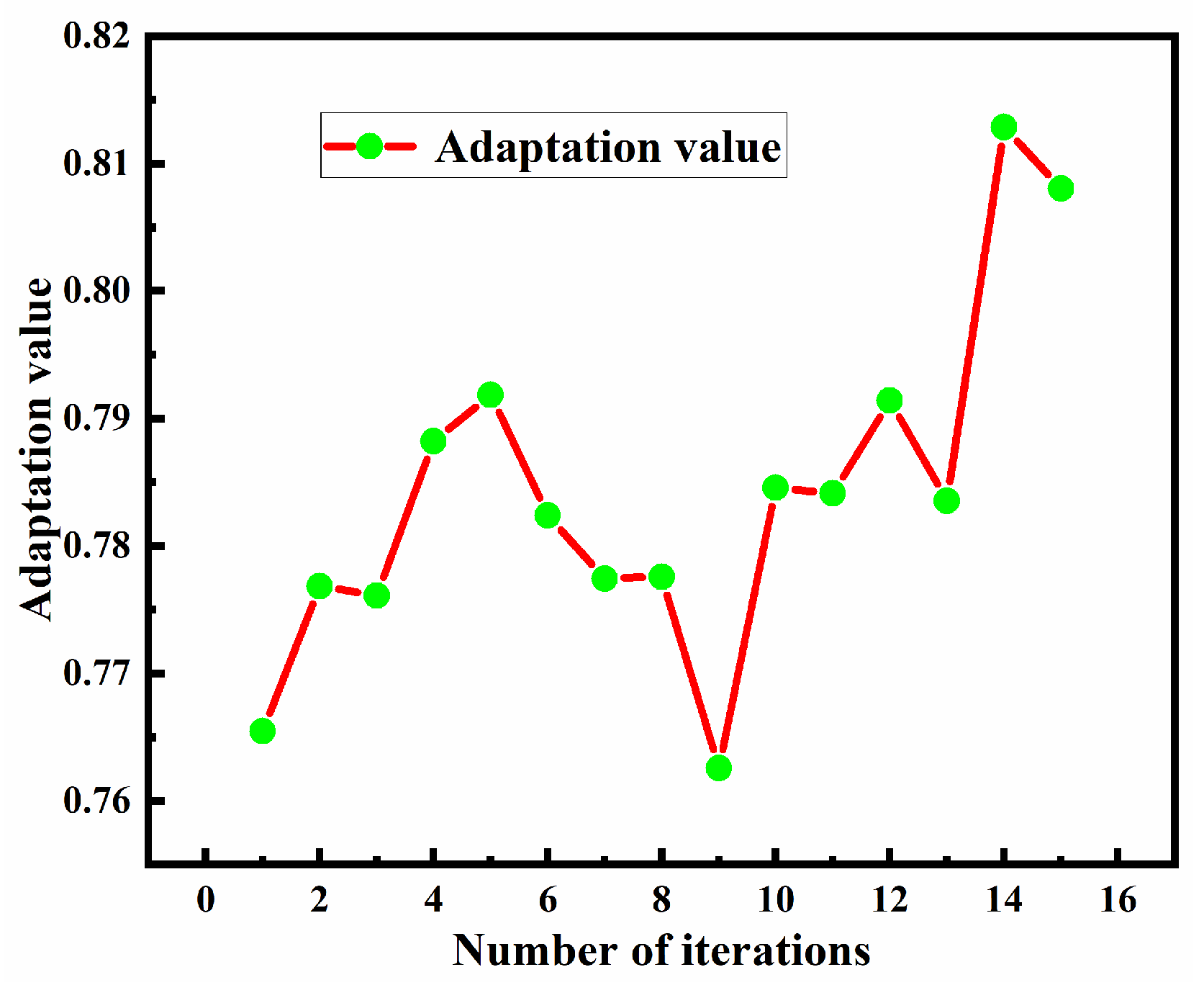
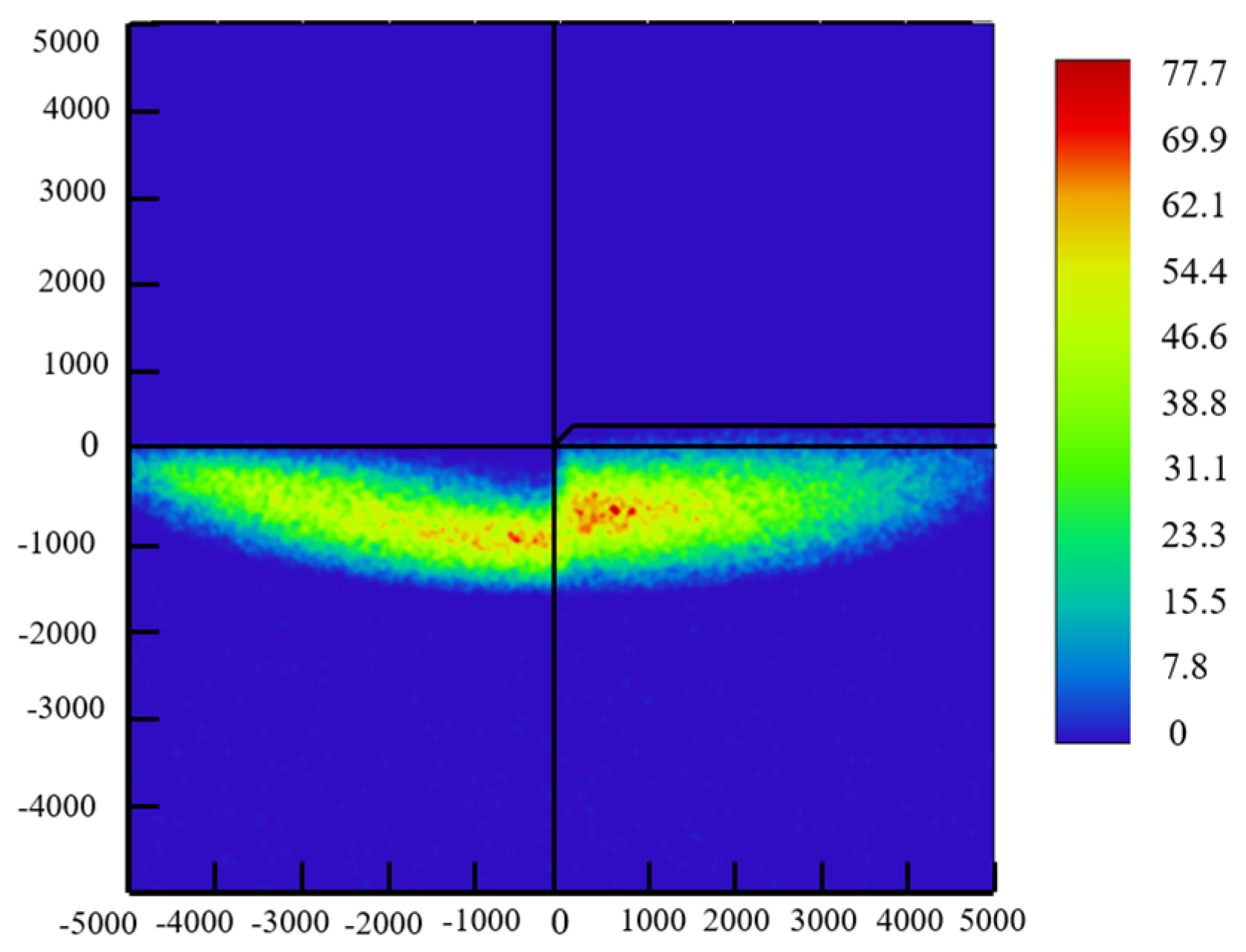
4.3. Results and Analyses

The optimization can be attributed to single-parameter genetic algorithm optimization. Referring to related literature, the number of individuals in the population of Jiang is generally set to 10–25, and the number of genetic generations is set to 10–20 times [25]. Given the intricacy of the model, the number of individuals in the population is set to 20, and the number of genetic generations is set to 15 in the simulation of this paper. To facilitate the genetic algorithm iteration of ZEMAX, a communication channel was established between MATLAB and ZEMAX, and the MATLAB code was written to implement this iteration.

According to the results obtained after the iteration, it can be observed that when the number of iterations reaches 14, the fitness level attains its maximum value in Figure 25. At this juncture, it can be posited that the parameter of the population aggregation prior to and following the 14th iteration constitutes the optimal solution for the specified objective. The results from the fifteenth iteration will be examined. A thorough examination of the error of the simulation reveals that in the population aggregated at ${\theta }_{max}$ = 2.2 in the 15th generation, the evaluation function of the individuals is situated in the uppermost interval. Based on Figure 26, the fitness level is recorded as 0.8. Subsequent to incorporating the value of ${\theta }_{max}$ = 2.2 into the computation of ${\theta }_{max}$, as detailed in Section 2 and Section 4, the optimal values of the high and low beam free-form mirrors are determined, as illustrated in Figure 27.

Then, the optical tracing simulation was carried out in ZEMAX to obtain its simulated light Figure 28, and the light values of each test point and test area as shown in

Table 4. The results of the optimized high-beam headlight.

Test Points or Areas	Required Illuminance (lx)	Simulated Illuminance (lx)
$E_{max}$	≥48 and ≤250	127.4
HV Point	≥$0.8 E_{max}$	110.4
1125L to HV and HV to 1125R	≥24	87.90
2250L to HV and HV to 2250R	≥6	38.62

.

The $E_{max}$ values are within the range of 48 lx to 250 lx, as stipulated by the standard. Furthermore, the illuminance at point HV exceeds 0.8 Emax. The minimum illuminance value at HV points 1125L and 1125R is 87.90 lx, while the minimum illuminance value at HV points 2250L and 2250R is 38.62 lx. These values satisfy the design requirements and are comparable with the values of each test point or area before optimization. The illuminance values of each test point or area have been enhanced in comparison to those observed before optimization. The luminous efficacy of the aforementioned device is 80.69%, and it is capable of achieving better optical uniformity, thereby avoiding the occurrence of high illuminance in the center and improving the global illuminance simultaneously. The length is 218.94 mm, the width is 101.14 mm, the height is 90.82 mm, and the optical efficiency is 89.40%. In comparison to the high beam obtained in Section 3, the length has been extended by 61.16 mm, the width by 40.79 mm, and the height by 20.93 mm, while the optical efficiency has been improved by 8.71%.

The shape of the low-beam is shown in Figure 29.

Subsequently, an optical tracing simulation is conducted in ZEMAX, as presented in Figure 30. The light values of each test point and test area are presented in

Table 5. The simulation results of the low-beam headlight.

Test Points or Areas	Simulated Illuminance (lx)	Fulfillment of Requirements
HV	0.5	Yes
B50L	0	Yes
75R	42.64	Yes
75L	10.73	Yes
50L	14.83	Yes
50R	49.07	Yes
50V	36.72	Yes
25L	10.94	Yes
25R	9.63	Yes
III area	≤0.46	Yes
VI areas	≥7.95	Yes
I areas	≤69.88	Yes

.

The dimensions of the headlight are as follows: length 255.72 mm, width 105.81 mm, height 96.04 mm. The optical efficiency is 88.89%. In comparison with the low-beam headlight previously described, the length was increased by 76.64 mm, the width by 43.13 mm, and the height by 23.13 mm, while the optical efficiency was improved by 8.30%.

It can be observed that the design of the low beam and high beam conforms to the specifications outlined in the national standard. To achieve a compact size while maintaining high optical efficiency, the design of this paper’s headlight outperforms that of conventional automotive headlights.

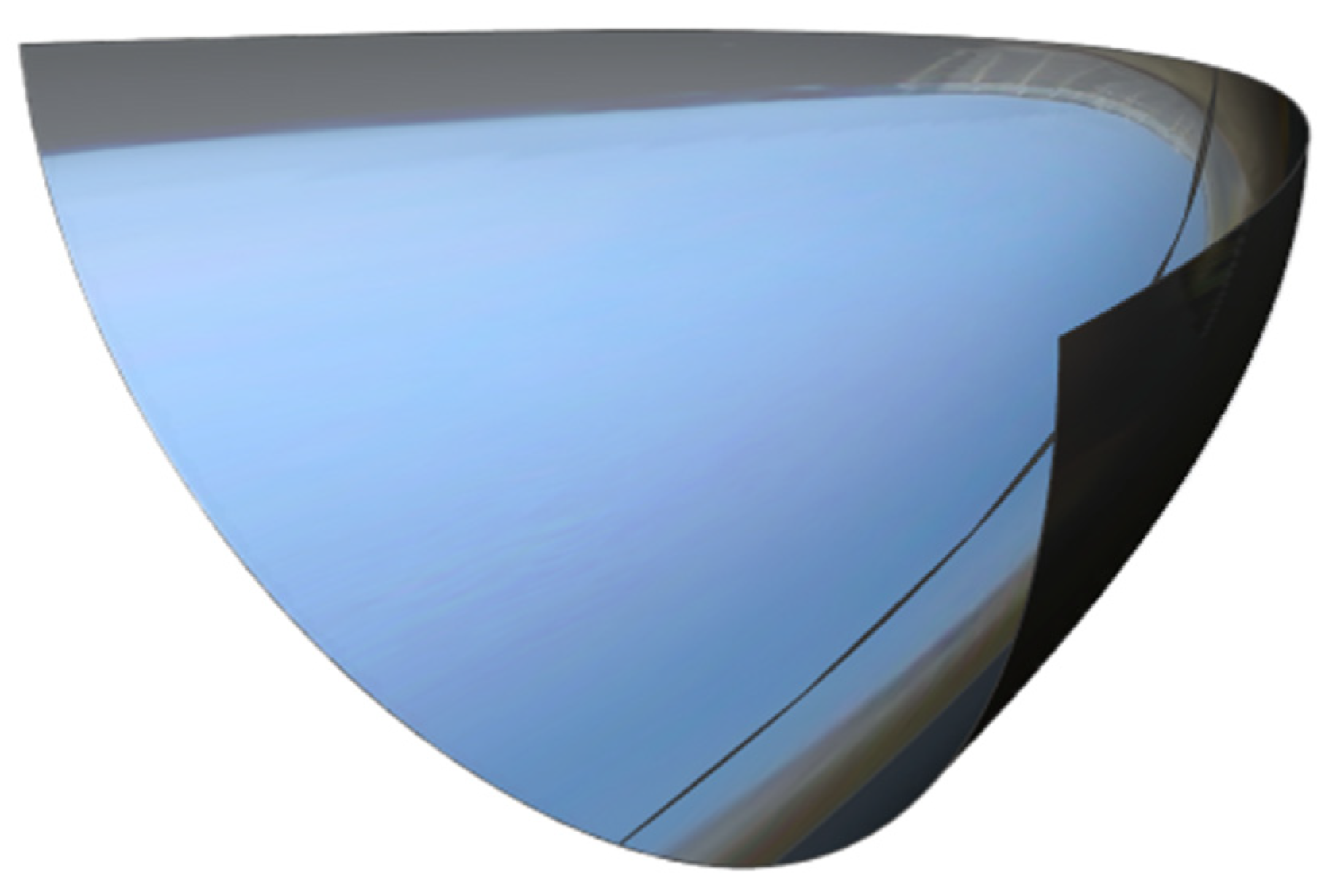
4.4. Manufacturing Process of Automotive Freeform Mirrors

The manufacturing of automotive headlight mirrors comprises three primary processes: injection molding, painting, and aluminizing. Compared to the manufacturing of conventional lamps, free-form lamp manufacturing entails increased costs associated with mold fabrication. Conversely, injection molding facilitates mass production, thereby enhancing the efficiency and cost-effectiveness of automotive headlamp manufacturing. The current processing of free-form surfaces primarily utilizes ultra-precision turning, and the polishing of the molds post-SPDT cutting necessitates the implementation of computer-controlled optical surface polishing (CCOS) and magnetorheological polishing (MRF) to enhance the surface finish [26,27].

Following injection-molding, the product surface is coated with primer to meet the stipulated surface finish requirements. Aluminizing fulfills the reflectivity requirement. The purpose of aluminizing is to improve the light reflection effect and decorative effect, which is 90% for aluminum and 90% for silver. Aluminum is a relatively economical and widely used material. The quality of the aluminized plate is a critical factor in determining light reflection [28].

5. Conclusions

In this paper, we initiate the study by employing the grid mapping method. We then introduce a control function that governs the illumination of the target surface. We subsequently complete the design and evaluation of the low beam and free-form surface. Following this, we establish an optimization model and optimize the design parameters using a genetic algorithm. This allows the reflector to achieve a balance between volume and luminous efficacy. The optimal θ_max is incorporated into the design of the low and high beams, and the final results are simulated. The comparison of the before and after design is shown in

Table 6. Comparison of results.

	Before Optimization		After Optimization
	High Beam	Low Beam	High Beam	Low Beam
${\theta }_{max}$ (rad)	2.09		2.2
dimension (mm)	157.78 × 60.35 × 69.89	179.08 × 62.08 × 72.91	218.94 × 101.14 × 90.82	255.72 × 105.81 × 96.04
efficiency (%)	80.69	80.59	89.40	88.89

, which demonstrates that according to our proposed method, the volume can be controlled within a reasonable range while ensuring high efficiency. In light of the accelerated development of new energy vehicles, there will be an increase in the use of LED lamps, and the design of LED lamps will continue to evolve. This paper proposes a free curved front lighting design and optimization method that can take into account optical efficiency and volume. This method better achieves uniform illumination while meeting design requirements and providing a reference for the uniformity of the light.

References

1. Hu, C.C.; Zheng, Y.J.; Hsu, Y.F.; Ye, Z.T. Design and Application of Liquid Silicone Rubber Light Guide in Compact Automotive Headlamps. Int. J. Optomechatron. 2024, 18, 2343407. [Google Scholar] [CrossRef]
2. Qin, R.S. New Trends in Accounting Reform and Development in the ‘14th Five-Year Plan’ Period. XinLiCai 2021, 9, 12–17. [Google Scholar]
3. Zhang, H.; Liu, D.; Wei, Y.; Wang, H. Asymmetric double freeform surface lens for integrated LED automobile headlamp. Micromachines 2021, 12, 663. [Google Scholar] [CrossRef] [PubMed]
4. Liu, L.; Lin, L. Design of a new pixel LED automobile headlamp. In Proceedings of the 2021 International Conference on Optical Instruments and Technology: Optical Systems, Optoelectronic Instruments, Novel Display, and Imaging Technology, Online, 8–10 April 2022; pp. 140–146. [Google Scholar]
5. Zhu, Z.; Wei, S.; Liu, R.; Hong, Z.; Zheng, Z.; Fan, Z.; Ma, D. Freeform surface design for high-efficient LED low-beam headlamp lens. Opt. Commun. 2020, 477, 126269. [Google Scholar] [CrossRef]
6. Siddula, S. Design of Modern Technology Lighting System for Automobiles Check for updates. Emerg. Technol. Sustain. Dev. Sel. Proc. EGTET 2023, 2022, 1061. [Google Scholar]
7. Zeng, Y. Free-form Automotive Laser Headlight Lighting System Based on Free-form Surface Design. Master’s Thesis, Changchun University of Science and Technology, Changchun, China, 2021. [Google Scholar]
8. Xie, S.S. Design and Performance Analysis of Automobile Headlamp Based on Light-Emitting Diode. J. Nanoelectron. Optoelectron. 2023, 18, 1203–1210. [Google Scholar] [CrossRef]
9. Bielawny, A.; Schupp, T.; Neumann, C. Automotive lighting continues to evolve. Opt. Photonics News 2016, 27, 36–43. [Google Scholar] [CrossRef]
10. Feng, Z.X.; Froese, B.D.; Liang, R.G.; Cheng, D.; Wang, Y. Simplified freeform optics design for complicated laser beam shaping. Appl. Opt. 2017, 56, 9308–9314. [Google Scholar] [CrossRef] [PubMed]
11. Yang, Y.S.; Qiu, D.; Zeng, Y.; Li, R.; Duan, W.; Fan, R. Design of a reflective LED automotive headlamp lighting system based on a free-form surface. Appl. Opt. 2021, 60, 8910–8914. [Google Scholar] [CrossRef] [PubMed]
12. Wang, H.; Chen, Z.J.; Wu, H.; Ge, P. Free-form LED automotive front-illuminated optical lens design method. Infrared Laser Eng. 2014, 43, 1529–1534. [Google Scholar]
13. Hsieh, C.C.; Tsai, C.L.; Hung, C.C.; Lin, H.H.; Li, T.C. Design of Multi-module LED Headlamp of Vehicle Under Federal Motor Vehicle Safety Standard. Sens. Mater. 2023, 35, 2433–2488. [Google Scholar] [CrossRef]
14. Alfred, M.; Hossein, A. Folded light source: A technique for compact and efficient automotive lighting. Opt. Eng. 2023, 62, 095104. [Google Scholar]
15. GB 25991-2010; Automotive Headlamps with LED Light Sources and/or LED Modules. Standardization Administration of China (SAC): Beijing, China, 2022.
16. Oshima, R.; Masashige, S. Study of LED Spot Beam lighting for Headlights. In Proceedings of the 2019 IEEE International Conference on Consumer Electronics (ICCE), Las Vegas, NV, USA, 11–13 January 2019. [Google Scholar]
17. Tsai, C.Y. Design of free-form reflector for vehicle LED low-beam headlamp. Opt. Commun. 2016, 372, 1–13. [Google Scholar] [CrossRef]
18. Wu, H.; Zhang, X.M.; Ge, P. Design method of a light emitting diode front fog lamp based on a freeform reflector. Opt. Laser Technol. 2015, 72, 125–133. [Google Scholar] [CrossRef]
19. Wang, L.P.; Su, P.; Ma, J.; Huang, J. LED high-beam module design for automotive headlight. AOPC 2021 Disp. Technol. 2021, 12063, 20–27. [Google Scholar]
20. Mas, A.; Martín, I.; Patow, G. Heuristic driven inverse reflector design. Comput. Graph. 2018, 77, 1–15. [Google Scholar] [CrossRef]
21. Tan, M.Y.; Chen, J. Dynamical optimized lamps distribution based on genetic algorithm for visible light communications. In Proceedings of the Eleventh International Conference on Information Optics and Photonics, Xi’an, China, 20 December 2019; pp. 1016–1021. [Google Scholar]
22. Brunnstrom, K.; Andrew, J.S. Genetic algorithms for free-form surface matching. In Proceedings of the 13th International Conference on Pattern Recognition, Vienna, Austria, 25–29 August 1996; pp. 689–693. [Google Scholar]
23. Shewchuk, J.R. Delaunay refinement algorithms for triangular mesh generation. Comput. Geom. 2002, 22, 21–74. [Google Scholar] [CrossRef]
24. Rahbek, L.W.; Kirkegaard, P.H.; Alibrandi, U. Parametric grid mapping design tool for freeform surfaces using a genetic algorithm. Proc. IASS Annu. Symp. 2020, 22, 1–12. [Google Scholar]
25. Lu, S.T. Characterization of Fabric Moisture Absorption and Quick-Drying Based on Segmentation Genetic Algorithm. Master’s Thesis, Zhongyuan University of Technology, Zhengzhou, China, 2023. [Google Scholar]
26. Li, X.L. Research on the Key Technology of Magnetorheological Polishing of Complex Curved Aluminum Mirror. Master’s Thesis, National University of Defense Technology, Changsha, China, 2018. [Google Scholar]
27. Xu, C.; Peng, X.Q.; Dai, Y.F. Current status of ultra-precision manufacturing of complex curved aluminum reflectors. Opto-Electron. Eng. 2020, 47, 200147. [Google Scholar]
28. Xie, Y.J.; Mao, X.L.; Li, J.P.; Wang, F.; Wang, P.; Gao, R.; Li, X.; Ren, S.; Xu, Z.; Dong, R. Optical design and fabrication of an all-aluminum unobscured two-mirror freeform imaging telescope. Appl. Opt. 2020, 59, 833–840. [Google Scholar] [CrossRef] [PubMed]
Figure 1. Lighting requirements of the low-beam headlight.
Photonics 12 00388 g001
Figure 2. Schematic diagram of latitude and longitude divisions: (a) front view; (b) top view.
Photonics 12 00388 g002
Figure 3. Schematic diagram of light source division.
Photonics 12 00388 g003
Figure 4. The design scheme: (a) the separation of mirrors on the left and right; and (b) the separation of target surfaces on the left and right.
Photonics 12 00388 g004
Figure 5. Energy analysis on the left side of the low-beam headlight.
Photonics 12 00388 g005
Figure 6. Fitting the control function for the left side of the low-beam.
Photonics 12 00388 g006
Figure 7. Energy analysis on the right side of the low-beam headlight.
Photonics 12 00388 g007
Figure 8. Fitting the control function for the right side of the low-beam.
Photonics 12 00388 g008
Figure 9. Schematic diagram of the low-beam light mapping path.
Photonics 12 00388 g009
Figure 10. Schematic diagram of the methodology employed for the calculation of a freeform surface: (a) the construction of the surface itself; and (b) the construction of the curve.
Photonics 12 00388 g010
Figure 11. Calculation results of the free-form discrete points: (a) discrete points on the left side of the reflector; (b) discrete points on the right side of the reflector.
Photonics 12 00388 g011
Figure 12. The designed low-beam headlight model.
Photonics 12 00388 g012
Figure 13. Schematic diagram of the simulated optical system.
Photonics 12 00388 g013
Figure 14. Simulation result of the low-beam headlight.
Photonics 12 00388 g014
Figure 15. Schematic diagram of energy loss.
Photonics 12 00388 g015
Figure 16. Lighting requirements of the high-beam headlight.
Photonics 12 00388 g016
Figure 17. Schematic diagram of the target surface division.
Photonics 12 00388 g017
Figure 18. Fitting the control function for the high-beam.
Photonics 12 00388 g018
Figure 19. Schematic diagram of the high-beam light mapping path.
Photonics 12 00388 g019
Figure 20. The designed freeform-based high-beam headlight model.
Photonics 12 00388 g020
Figure 21. Simulation result of the high-beam headlight.
Photonics 12 00388 g021
Figure 22. Volume–efficiency.
Photonics 12 00388 g022
Figure 23. The construction process of an STL solid model: (a) YOZ 2D point cloud, (b) triangular sectioning, and (c) mesh construction.
Photonics 12 00388 g023
Figure 24. Optimization flow chart of the headlight structure.
Photonics 12 00388 g024
Figure 25. The distribution of individuals in the fifteenth generation.
Photonics 12 00388 g025
Figure 26. Variation of the best solution per generation.
Photonics 12 00388 g026
Figure 27. The optimized high-beam headlight model.
Photonics 12 00388 g027
Figure 28. The optimized lighting map of the high-beam headlight.
Photonics 12 00388 g028
Figure 29. The optimized low-beam headlight model.
Photonics 12 00388 g029
Figure 30. The optimized lighting map of the low-beam headlight.
Photonics 12 00388 g030