Defect Detection Method for Large-Curvature and Highly Reflective Surfaces Based on Polarization Imaging and Improved YOLOv11

Abstract

In industrial manufacturing, product quality is of paramount importance, as surface defects not only compromise product appearance but may also lead to functional failures, resulting in substantial economic losses. Detecting defects on complex surfaces remains a significant challenge due to the variability of defect characteristics, interference from specular reflections, and imaging non-uniformity. Traditional computer vision algorithms often fall short in addressing these challenges, particularly for defects on highly reflective curved surfaces such as aircraft engine blades, bearing surfaces, or vacuum flasks. Although various optical imaging techniques and advanced detection algorithms have been explored, existing approaches still face limitations, including high system complexity, elevated costs, and insufficient capability to detect defects with diverse morphologies. To address these limitations, this study proposes an innovative approach that analyzes the propagation of light on complex surfaces and constructs a polarization imaging system to eliminate glare interference. This imaging technique not only effectively suppresses glare but also enhances image uniformity and reduces noise levels. Moreover, to tackle the challenges posed by the diverse morphology of defects and the limited generalization ability of conventional algorithms, this study introduces a novel multi-scale edge information selection module and a Focal Modulation module based on the YOLOv11 architecture. These enhancements significantly improve the model’s generalization capability across different defect types. Experimental results show that, compared to state-of-the-art object detection models, the proposed model achieves a 3.9% increase in precision over the best-performing baseline, along with notable improvements in recall, mAP50, and other key performance indicators.

1. Introduction

In industrial production, defects often arise on product surfaces due to issues in manufacturing processes and techniques. In severe cases, these defects can result in product failure and significant economic losses. Currently, surface defect detection methods include laser inspection [1], eddy current testing [2], infrared detection [3], and machine vision-based detection [4]. Among these, machine vision-based detection is the most widely applied and has been extensively used for detecting defects on steel surfaces [5], integrated circuits [6], and cylindrical batteries [7]. However, detecting defects on complex curved surfaces using vision-based methods still faces several challenges. First, specular reflection on smooth surfaces can cause glare interference, causing overexposure and distortion in certain image regions, which results in the loss of defect information in those areas. Second, the morphology of surface defects varies depending on their location on the curved surface, leading to instability in defect shapes [8]. Additionally, surface defects are often small in scale [9], exhibit inconspicuous features, and have diverse morphologies, making them difficult to extract. Traditional vision algorithms, such as edge detection [10], filtering methods [11], and texture-based algorithms [12], lack the generalization ability to handle defects of varying scales and forms. When surface defects such as scratches, cracks, and rust appear on complex curved surfaces, such as aircraft engine blades [9], bearing surfaces [13], ceramic surfaces [14], and thermos cup surfaces, they may shorten the product’s lifespan or even lead to failure, posing safety hazards and the risk of accidents.

Many researchers have conducted studies on optical imaging and detection algorithms for complex curved surfaces. Zhou et al. [15] Employed dual strip backlights to illuminate both sides of highly reflective chrome-plated parts and fused the two images to reconstruct the surface profile. However, this separate illumination and fusion method is only effective for defects with certain surface undulations, such as scratches. When the object surface has surface contamination present or the defect undulations are subtle, the detection performance deteriorates. Xu et al. [16] proposed a defect detection method based on polarized light filtering, where they mathematically modeled the light propagation process and intensity loss. They suppressed image noise and enhanced defect contrast by leveraging polarization filtering. However, their experiments were conducted on simple cylindrical smooth surfaces, lacking research on imaging complex surfaces with varying curvatures. Wei et al. [17] utilized a digital micromirror device (DMD) to implement a pixel-level spatiotemporal modulation method for adaptive illumination in vision imaging, effectively suppressing halo interference and strong specular reflections on the object’s surface. However, the use of DMD for pixel-level spatiotemporal modulation increases system complexity, requiring precise light source control and real-time feedback. This high complexity may lead to increased costs, making large-scale industrial applications less feasible. Meng et al. [18] employed Gray codes and a four-step phase-shifting method to determine the absolute phase of reflected images. They used an absolute phase gradient transformation method and affine transformation for posture correction, while template matching was applied for detecting diffuse reflection surface defects. Additionally, grayscale morphological opening and closing operations were performed on the original images to obtain defect shape and position information, thereby identifying image defects. However, on complex surfaces or at defect edge regions, reflected light may undergo multiple reflections or occlusions, leading to irregular phase variations, which in turn affect the accuracy of defect detection. Chen et al. [19] proposed a novel method for the imaging and edge detection of internal delamination defects in carbon fiber reinforced polymers (CFRP) using continuous line laser scanning excitation. Their Flash Laser Scanning Thermography (FLST) system captured thermal images and reconstructed the infrared images of defects using simple feature lines, while the effects of different parameters on the reconstructed images were analyzed. Finally, the morphological characterization of internal delamination defects in CFRP was achieved through a motion blur removal method combined with an edge detection algorithm. The results indicated that this method demonstrated high accuracy and efficiency in the non-destructive testing and evaluation of delamination defects.

High-precision optical imaging systems have laid a solid foundation for industrial inspection. However, in complex curved surface scenarios, accurate defect extraction on complex curved surfaces still faces two major challenges. First, defects are randomly distributed across curved surfaces, and their shapes can vary significantly depending on their location due to the varying geometry of the curved surface. This morphological diversity greatly increases the difficulty of defect extraction. Second, defects appear at multiple scales. Some defects are physically much smaller than the background region, resulting in a low signal-to-background ratio in the image, which raises the likelihood of missed detections. In contrast, larger defects with weak semantic features may be misclassified as background elements during feature extraction, also leading to detection errors. Currently, there are numerous defect extraction methods based on traditional vision algorithms. For instance, Bao et al. [20] designed a machine vision-based defect detection system for the surface of cylindrical rollers in bearings. By applying Otsu threshold segmentation, Canny edge detection, and morphological processing, they extracted and identified surface defects on rollers, classifying and labeling them accordingly. Wang et al. [21] proposed a dual-channel feature fusion-based vision detection method for the rapid detection of wheel hub cracks. Zheng et al. [22] introduced a method based on multi-wavelet transform and autoencoder networks for defect matching on steel surfaces. Liu et al. [23] developed a hybrid recognition method combining mathematical morphology and pattern recognition for defect detection on PCB surfaces.

In parallel, a wide range of defect detection methods based on deep learning have emerged, driving significant progress in object detection networks. These include single-stage object detection networks such as the YOLO series [24] and two-stage detection networks like Faster R-CNN [25]. However, deep learning-based defect detection often faces challenges such as sample imbalance and the difficulty of detecting small targets [26]. To address the challenge of small object detection in defect detection, subsequent researchers have integrated attention mechanisms and multi-scale feature fusion into neural networks to enhance their ability to detect small defects. Song et al. [27] proposed an cross-layer semantic guided network (CSGNet) based on YOLOv6 to detecting defects in small aero-engine blades. Zhao et al. [28] designed a defect detection model for turbine blades based on ShuffleNetV2 and Coordinate Attention. Li et al. [29] proposed a deep convolutional neural network (DCNN) for detecting surface defects on aero-engine blades. Liu et al. [30] introduced Bearing-DETR, an optimized deep learning model based on the RT-DETR architecture for bearing defect detection. Fei et al. [31] proposed TinyDefectNet, a specialized deep ensemble learning algorithm for the online identification of micro-defects in large images acquired from dedicated image acquisition modules.

To tackle the technical challenges associated with defect detection on complex curved surfaces, this study proposes several innovative solutions. First, the imaging of such surfaces is highly prone to specular glare, which can obscure critical defect information. To overcome this, polarized imaging technology is employed to suppress glare interference, thereby improving the signal-to-noise ratio of defect features. Second, to mitigate defect shape distortion induced by the geometric complexity of curved surfaces, a multi-scale edge information selection architecture is introduced to enhance the model’s adaptability to morphologically diverse defects. Furthermore, a spatial pyramid pooling module is integrated to capture cross-scale contextual information, enriching the semantic representation and improving detection robustness.

2. Method

To address the challenges of glare interference and morphological diversity in defect detection on complex curved surfaces, this study proposes a dual-level solution that integrates polarization imaging with deep learning optimization. At the optical imaging level, polarization imaging technology is utilized, where polarizers are employed to filter out glare predominantly composed of polarized light, while retaining randomly scattered diffuse reflections that accurately convey the surface characteristics of curved objects. At the algorithmic level, a multi-scale edge information selection (MSIS) module and a Focal Modulation module are embedded into the YOLOv11 architecture. By leveraging a parallel-branch network to extract edge features across multiple scales, coupled with an adaptive weighting mechanism for effective multi-scale feature fusion, the proposed method significantly improves the model’s capacity to detect defects of varying morphologies on complex surfaces. Finally, a specialized dataset is constructed using polarization-filtered images with annotated defect labels, which is then used to train the enhanced MF-YOLOv11 model.

2.1. Polarization Imaging Principle

Uneven illumination on curved surfaces leads to variations in light reflection angles during imaging, resulting in inconsistent pixel intensities across different surface regions and increasing the difficulty of defect extraction. Moreover, reflective interference on smooth surfaces often generates glare, which can weaken or even obscure defect information in affected areas. Compared to conventional imaging techniques, polarization imaging offers distinct advantages in capturing material properties, surface roughness, and geometric features. This capability enhances the extraction of defect textures and structural details, thereby improving detection accuracy and robustness. The polarization state of light can be represented by the Stokes vector (I, Q, U, V), as defined in Equation (1). Here, I represents the total light intensity, Q denotes the intensity difference between horizontally and vertically polarized light, U represents the intensity difference between +45° polarized light and −45° polarized light, and V denotes the intensity difference between left- and right-handed circularly polarized light.

$$\left\{\begin{array}{c}I=I_{\mathrm{t}}\\ Q=(I_{0^{\circ }}-I_{{90}^{\circ }})\\ U=(I_{+{45}^{\circ }}-I_{-{45}^{\circ }})\\ V=(I_{rc}-I_{lc})\end{array}\right.$$

(1)

In this case, I_t represents the total light intensity, while I₀, I₄₅, I₉₀, and I₋₄₅ represent the intensity of polarized light at angles of 0°, 45°, 90°, and −45° to the horizontal direction, respectively. I_rc and I_lc represent the intensities of right circularly polarized and left circularly polarized light, respectively. The degree of linear polarization of light is defined by Equation (2) as follows:

$${\mathrm{y}}_{DoLP}={\displaystyle \frac{\sqrt{Q^2+U^2}}{I_t}}$$

(2)

When the light is completely composed of polarized light, the degree of linear polarization, calculated using Equation (2), is equal to one. On the other hand, the Stokes vector for natural light is represented as (I₀,0,0,0), with a linear polarization degree of zero. By adding a linear polarizer to the surface of the light source, the natural light emitted by the source can be converted into linearly polarized light. According to Malus’ law, the intensity of light after passing through the polarizer can be expressed by Equation (3):

$$I={\displaystyle \frac{1}{2\pi }}{\int }_0^{2\pi }{I}_{\theta }{\cos }^2\theta d\theta ={\displaystyle \frac{I_0}{2}}$$

(3)

From Equation (3), it can be observed that natural light, which has a completely random vibration direction, will have its intensity reduced to half of I₀ after passing through a polarizer, where I₀ is the total light intensity. At this point, the light is fully converted into linearly polarized light. According to electromagnetic theory and Fresnel’s law, when a light wave strikes the surface of a medium, its electric field vector can be decomposed into two orthogonal components: the s-component and the p-component. The s-component’s electric field direction is perpendicular to the incident plane, while the p-component’s electric field direction is parallel to the incident plane. The reflection coefficient r_s and transmission coefficient t_s for s-polarized light, as well as the reflection coefficient r_p and transmission coefficient t_p for p-polarized light, are defined in Equation (4).

$$\left\{\begin{array}{c}{r}_s={\displaystyle \frac{n_1\cos {\theta }_i-n_2\cos {\theta }_t}{n_1\cos {\theta }_i+n_2\cos {\theta }_t}}\\ t_s={\displaystyle \frac{2n_1\cos {\theta }_i}{n_1\cos {\theta }_i+n_2\cos {\theta }_t}}\\ r_p={\displaystyle \frac{n_2\cos {\theta }_i-n_1\cos {\theta }_t}{n_2\cos {\theta }_i+n_1\cos {\theta }_t}}\\ t_p={\displaystyle \frac{2n_1\cos {\theta }_i}{n_2\cos {\theta }_i+n_1\cos {\theta }_t}}\end{array}\right.$$

(4)

In Equation (4), n₁ denotes the refractive index of the incident medium, typically air, with a value of 1. n₂ represents the refractive index of the transmitted medium, set to 1.35 based on the common optical properties of curved materials. θ_i is the incident angle, and due to the light source’s alignment perpendicular to the surface, the incident angle is 90 degrees. θ_t is the refraction angle, which is 47.8 degrees. According to Equation (4), both polarization components exhibit 100% reflectance, and the transmittance is 0%. As the incident light is completely linearly polarized, the reflected light is also fully linearly polarized. However, because the light source is a planar source, it not only illuminates the surfaces perpendicular to itself but also those with varying orientations. In these cases, the incident angle is not 90 degrees, and thus the reflectance is less than 100%, and the transmittance is greater than 0%. Consequently, non-linearly polarized components, such as diffusely reflected or elliptically polarized light, appear on the object’s surface. These components retain random polarization states. The principle of the polarization imaging system is illustrated in Figure 1.

To suppress glare, primarily composed of linearly polarized light, while preserving useful surface information, a polarizer is employed to selectively block the linearly polarized component of reflected light and allow randomly or non-linearly polarized light to pass through. This effectively retains valuable image features. The underlying principle is illustrated in Figure 1. Given that the polarization direction of incident light is fixed, the linearly polarized portion of the reflected light tends to be more concentrated. By adjusting the rotation angle of the polarizer in front of the camera, the glare can be maximally attenuated, thereby enhancing the visibility of surface details on the object.

Therefore, a polarizer is first used to polarize the light emitted from the light source. Taking a horizontal polarizer as an example, the Stokes vector of the horizontally polarized light after polarization is represented as (I₀, I₀, 0, 0), indicating that the light remains horizontally polarized after reflecting off the object’s surface. In this stage, a vertical polarizer is placed in front of the imaging device. Since the vertical polarizer is orthogonal to the polarization direction of the incident light, the intensity of the transmitted light is significantly reduced. The transmitted intensity can be described by Equation (5):

$$I={\displaystyle \frac{1}{2}}(I_0+{\mathrm{Q}}_0{\cos }^2(\theta )+{\mathrm{U}}_0{\sin }^2(\theta ))$$

(5)

From Equation (5), it can be observed that since the angle θ between the horizontally polarized light and the vertical polarizer is 90 degrees, the glare caused by the horizontally polarized component is effectively filtered out. As a result, only a portion of the incident light—primarily consisting of diffusely reflected and elliptically polarized light—is transmitted. This remaining light effectively captures and preserves the surface characteristics of the complex curved object.

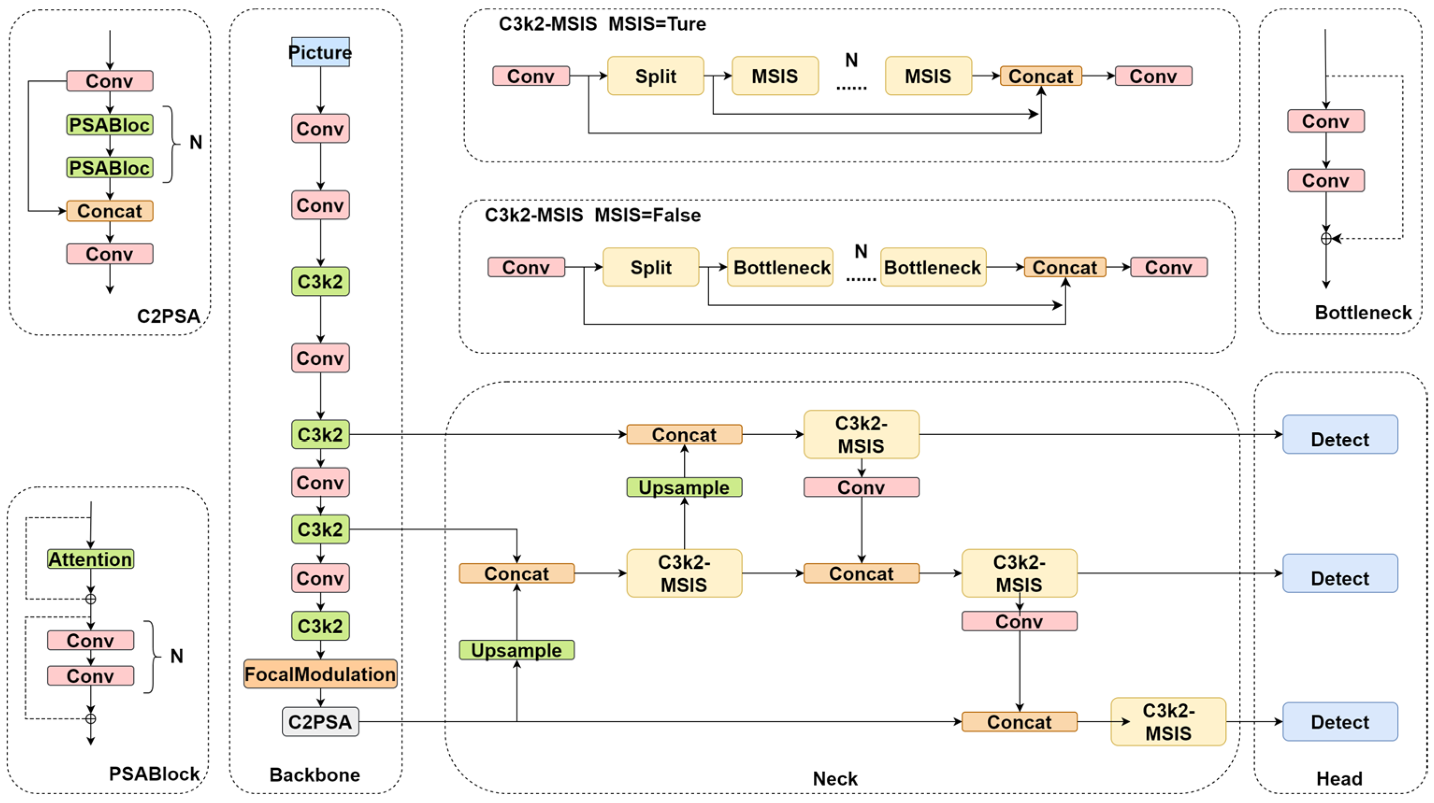
2.2. Improving the YOLOv11 Model

This study proposes the MF-YOLOv11 detection model to address the challenges of diverse defect morphologies, small defect scales, and indistinct defect features in defect detection for complex curved surfaces. The proposed model incorporates the following innovative modules: (1) A C3k2-MSIS module based on multi-scale edge information selection (MSIS) is used, which processes features through adaptive pooling at different scales and depthwise separable convolutional branches combined with an edge enhancement module to refine edge details. The model’s robustness is significantly improved by employing a dual-domain selection mechanism that balances spatial key region focusing and dynamic channel feature optimization. (2) The Focal Modulation module, which replaces the traditional SPPF module, is also used. This module leverages contextual relevance and a gating mechanism to dynamically assign weights, selectively aggregating key contextual information. This approach mitigates the indiscriminate fusion in conventional SPPF structures that often introduces noise interference, thereby enhancing the effectiveness of feature integration. Additionally, convolution kernels of different sizes are utilized to extract multi-scale features ranging from local to global levels, replacing traditional pooling operations to improve edge and detail capture capabilities. The improved MF-YOLOv11 structure is shown in Figure 2.

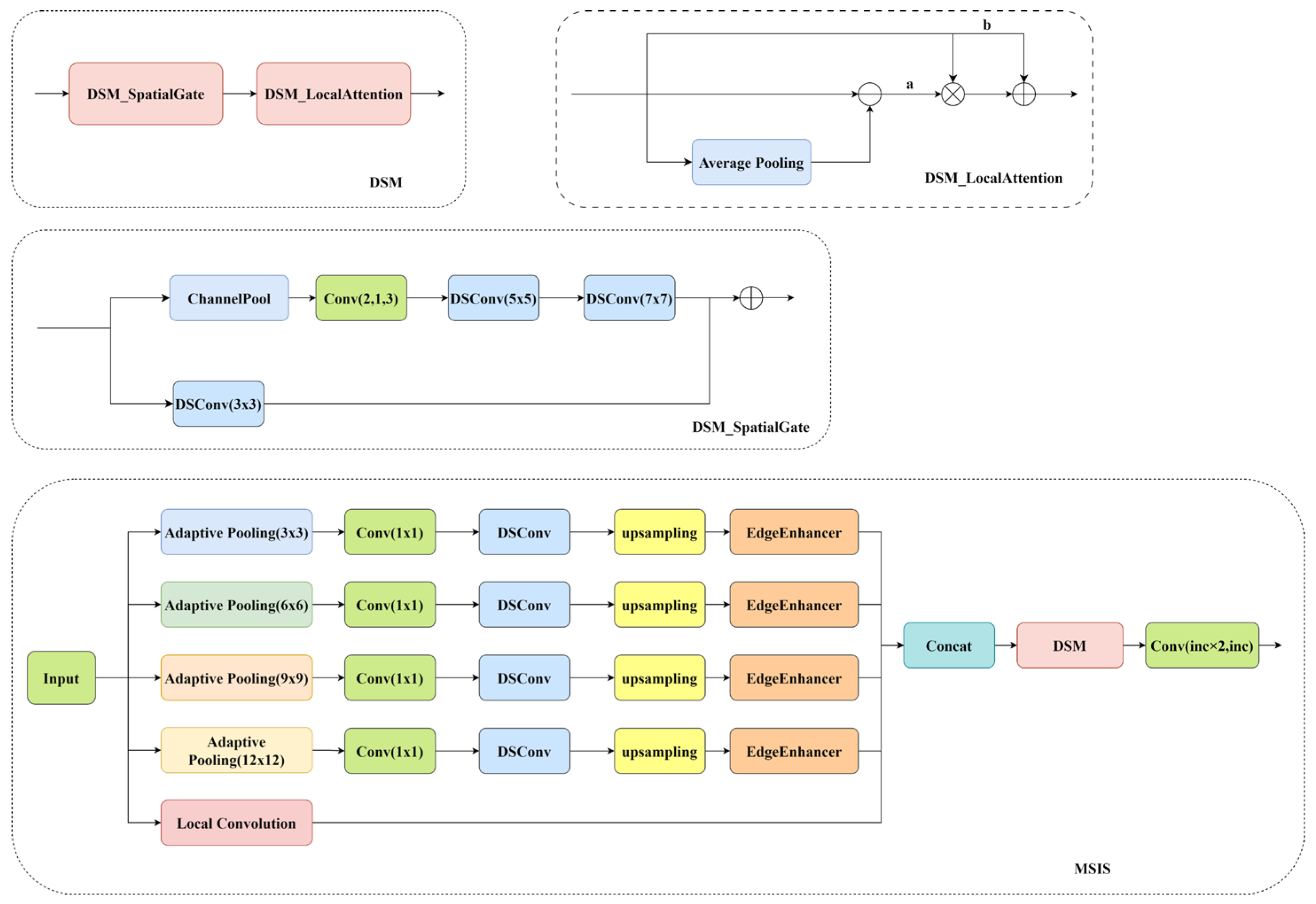
2.2.1. Multi-Scale Edge Information Selection Module

To enhance the network’s ability to extract multi-scale features, a multi-scale edge information selection (MSIS) module is introduced based on the original C3k2 module. The module framework is shown in Figure 3. The core principle of this module is to perform adaptive pooling at different scales on the input image, followed by depthwise separable convolution branches to process features at each scale. After feature upsampling, an edge enhancement module is applied to amplify the edge information in the feature map. The resulting feature maps are concatenated along the channel dimension and then passed through a dual-domain selection mechanism module to focus on key features in both the spatial and channel dimensions.

The edge enhancement module extracts the low-frequency information of the image through average pooling and subtracts this low-frequency information from the original input image x, thereby retaining the high-frequency information which corresponds to the edges. Simultaneously, the edge weight w is computed using a Sigmoid function. The edge information is then multiplied by the weight w and added back to the original input image x, enabling the preservation of the original information while emphasizing the edge details. The mathematical definitions of the overall process are given by Equations (6) and (7).

$$output=x+w(x-AvgPool(x))$$

(6)

$$w={\displaystyle \frac{1}{1+e^{-(x-AvgPool(x))}}}$$

(7)

The dual-domain selection mechanism (DSM) consists of the spatial-domain selection module and the channel-domain selection module. The spatial-domain selection module utilizes a stacked structure of 5 × 5 and 7 × 7 convolutional kernels to capture structural information from the image, along with a 3 × 3 convolutional kernel to capture local detail information. Subsequently, global average pooling and global maximum pooling are performed in parallel on the input feature map, and their outputs are concatenated along the channel dimension to form a 2-channel feature that contains global statistical information. A subsequent 1 × 1 convolution layer is used to aggregate the 2 channels and generate a spatial attention weight map. This weight map is then multiplied by the image’s structural information and added to the original local detail information through a residual connection.

The channel threshold selection module begins by initializing learnable weights a and b, which enable the adaptive adjustment of the channel features. The mean value of the spatial dimensions of the input feature x is then calculated to obtain a reference value that represents the global features. Subsequently, the input feature x is subtracted from this mean value to obtain the feature deviation out, establishing a weighted residual connection structure. The specific definition of this process is provided in Equation (8).

$$output=a\times out\times x+b\times x$$

(8)

The learnable weights a and b dynamically adjust the fusion ratio between the original features and the feature deviation, enhancing the model’s ability to represent feature distribution shifts while preserving the original feature information.

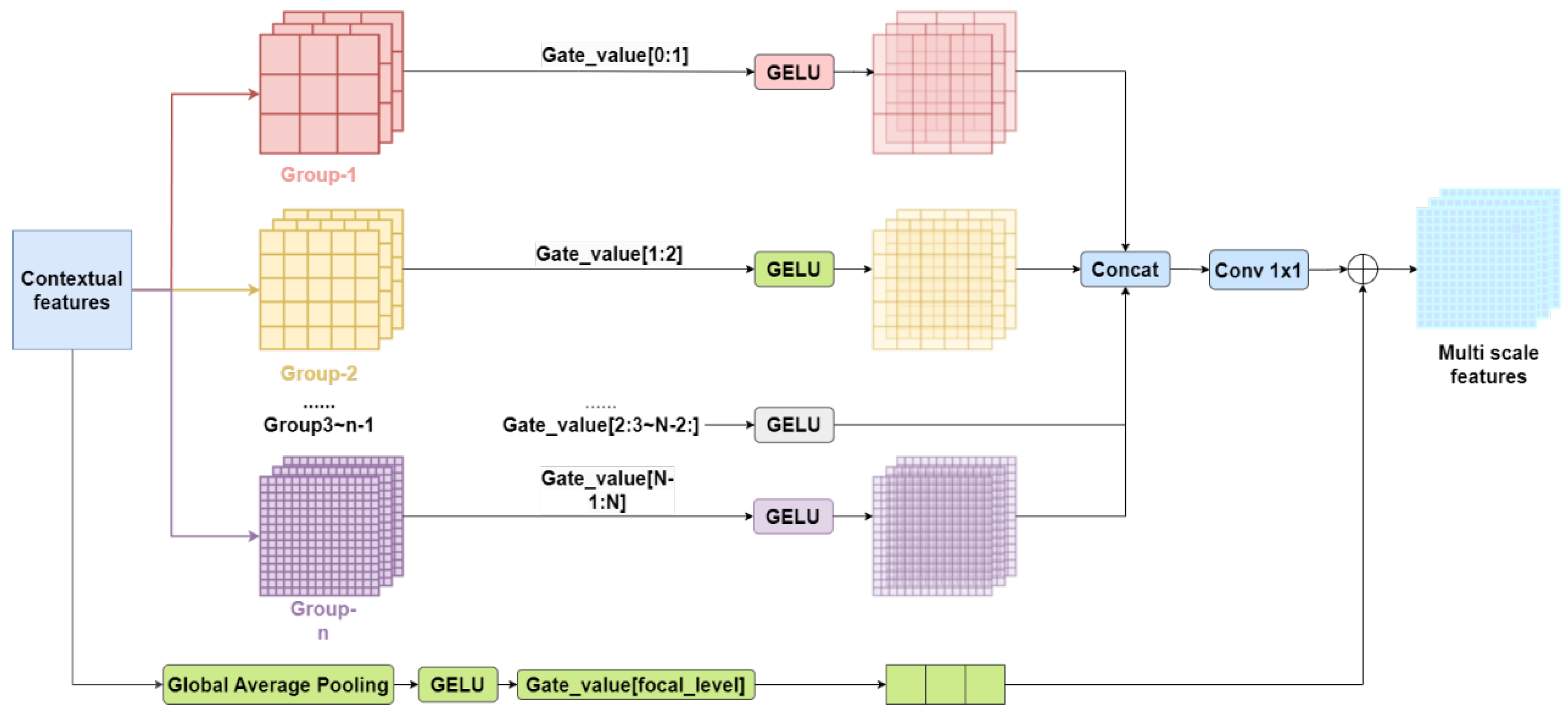
2.2.2. Focal Modulation Module

The core principle of the Focal Modulation module is hierarchical context extraction and dynamic gating mechanism. Its function is to replace the self-attention mechanism by utilizing depthwise separable convolutions to capture multi-scale visual context information from local to global scale. The gating mechanism then dynamically aggregates key contextual information, thereby reducing computational complexity while enhancing the model’s ability to perceive multi-scale features. The dynamic gating mechanism achieves the adaptive fusion of multi-scale features through dynamic weights g_l. The model principle of dynamic gating is illustrated in Figure 4.

Each group consists of convolutional kernels of different sizes, which are used to extract feature information at different scales. The extracted feature information is multiplied by the corresponding dynamic weight g_l and passed through a GELU activation function to introduce non-linearity. The approximate definition of the GELU activation function is given in Equation (9). The activated feature maps are then concatenated along the channel dimension, and multi-scale feature fusion is completed using a 1 × 1 convolution.

$$\mathrm{GELU}(x)=0.5x\left[1+\tanh \left(\sqrt{{\displaystyle \frac{2}{\pi }}}(x+0.047715x^3)\right)\right]$$

(9)

The green process box below Figure 4 indicates that the global average pooling is used to obtain the spatial mean of the contextual information, which is then added to the feature map after multi-channel feature fusion, resulting in the aggregated contextual information ctx_all. The expression is given in Equation (10).

$$ct{x}_{all}=\sum _{l=0}^{L-1}Con{v}_l(ctx)g_l+GAP(ctx)g_L$$

(10)

The Focal Modulation module demonstrates significant advantages over the traditional SPPF structure. Firstly, it replaces fixed-size pooling layers with hierarchical convolution, enabling more flexible multi-scale edge and detail feature extraction. Secondly, its gated aggregation mechanism emphasizes content relevance, effectively mitigating the noise interference caused by indiscriminate feature fusion in SPPF. Furthermore, Focal Modulation reduces the computational complexity from O(N²) in SPPF to a linear complexity of O(N), maintaining the capability of multi-scale feature fusion while significantly improving computational efficiency, which is particularly beneficial for high-resolution image processing tasks.

3. Experimental Results and Analysis

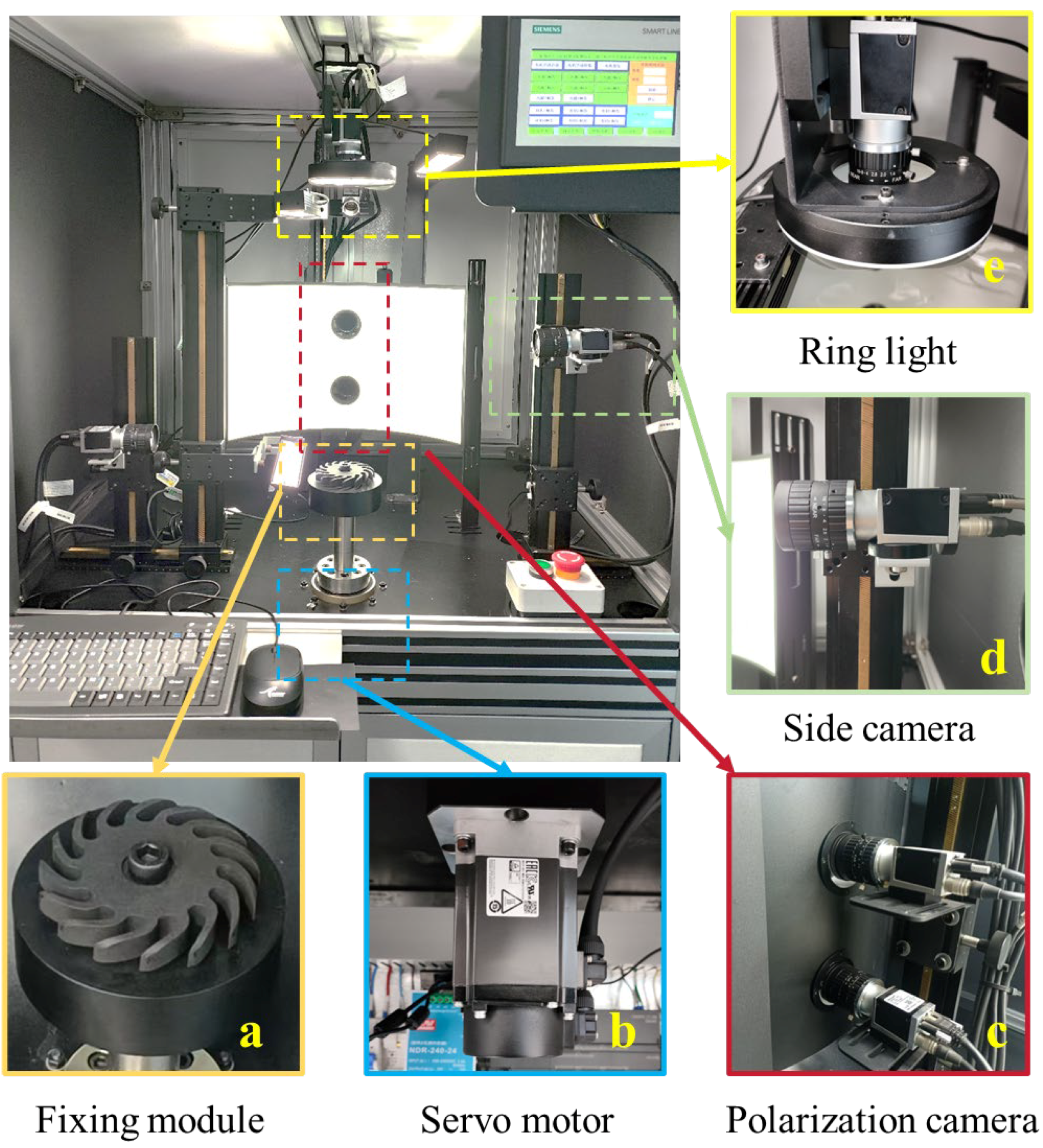
3.1. Test Equipment Construction

To verify the effectiveness of the proposed polarization imaging method and the enhanced MF-YOLOv11 model, a series of complex curved surface samples were fabricated for testing, and a dedicated inspection platform was constructed. The hardware configuration of the inspection platform is shown in Figure 5. It includes a rotational and fixation mechanism as well as multiple imaging modules. The detailed hardware specifications of the image acquisition unit are listed in

Table 1. Image acquisition module hardware composition.

Number	Device Name	Brand	Model
1	Camera	Basler, Ahrensburg, Germany	Aca-2500-30gc
2	Lenses	ZLZK, Zoomlion, Changsha, China	LM0820MP5
3	Light Source	V-Light, China	VLHBGLXD30X245B-24V
4	Industrial Computer	Hikvision, Hangzhou, China	MV-IPC-F487H
5	PLC	Siemens, Munich, Germany	S7-200 SMART
6	Frame grabber	Daheng Imaging, Beijing, China	PCIe-GIE72P

.

The fixation module, as illustrated in Figure 5a, is fitted with elastic friction pads on its outer surface. When a sample is placed and secured, the pads deform to provide both clamping force and friction, ensuring the stable fixation of complex curved surfaces. The servo motor, shown in Figure 5b, is installed beneath the inspection platform and connected to a reducer. The output shaft of the reducer is coupled with the fixation module, enabling the sample to rotate during a full circumferential scan. At the center of the inspection platform, a 400 mm × 600 mm arc-shaped light source is installed. Its light-emitting surface is covered by a polarizer of the same dimensions. Two through-holes are located at the center of the arc light source, allowing the polarization camera to capture images of the sample through them. As shown in Figure 5c, the polarization camera is mounted behind the arc light source on a supporting bracket. In addition, two side cameras are positioned on the left and right sides of the platform, as illustrated in Figure 5d. These cameras are used to detect non-planar defects on the sample surface. To ensure sufficient and uniform illumination, a ring light and two strip lights—mounted on either side of the ring—are employed, as shown in Figure 5e.

To obtain a complete image sequence of the sample, the servo motor rotates in 90° increments, briefly pausing in each step. During each pause, all imaging units simultaneously capture images of the sample. Once imaging is completed in the current position, the servo motor advances by another 90°, and the process repeats. This cycle continues until a full 360° image sequence of the sample is acquired.

3.2. Polarization Imaging Performance Experiment

To evaluate the effectiveness of polarization imaging, 100 raw images without polarization filtering and 100 images captured with polarization imaging for glare suppression were acquired using the equipment described in Section 3.1, under consistent lighting and camera settings. These images were compared against results obtained using the high dynamic range imaging (HDRI) algorithm, a commonly applied technique for defect detection on highly reflective metal surfaces. In the context of defect detection, image quality is primarily assessed using three key metrics: root mean square (RMS) noise, standard deviation, and the uniformity index.

The definition of root mean square (RMS) noise is given in Equation (11), where F(i, j) represents the test image and F’(i, j) represents the reference image, which is obtained by applying Gaussian low-pass filtering to the test image. The definition of Gaussian low-pass filtering is provided in Equation (12). Low-pass filtering effectively removes noise from the image. RMS noise reflects the intensity of the high-frequency noise removed; a higher value indicates a greater presence of high-frequency noise components in the original image, and consequently, a higher amount of noise energy removed after filtering.

$$\mathrm{RMS} \mathrm{Noise}=\sqrt{{\displaystyle \frac{1}{MN}}\sum _{i=1}^M\sum _{j=1}^N{\left(F(i,j)-F^{\prime }(i,j)\right)}^2}$$

(11)

$$G(x,y)={\displaystyle \frac{1}{2\pi {\sigma }^2}}{e}^{-{\displaystyle \frac{x^2+y^2}{2{\sigma }^2}}}$$

(12)

The definitions of image standard deviation and uniformity index are given in Equations (13) and (14), respectively. In Equation (13), u represents the mean grayscale value of the image. The standard deviation measures the degree of dispersion of pixel values relative to the mean grayscale value, reflecting the concentration or spread of pixel distributions. A lower standard deviation indicates a more concentrated pixel distribution, suggesting the effective removal of high-intensity glare interference. Conversely, a higher standard deviation indicates a more dispersed pixel distribution, implying the poor suppression of high-intensity glare interference. The uniformity index is calculated as the sum of the squared probabilities of each grayscale level and directly reflects the concentration of the grayscale distribution. A higher uniformity index indicates that the grayscale values are concentrated within a few levels, implying strong grayscale consistency in the captured image, which is beneficial for subsequent algorithmic processing. In contrast, a lower uniformity index suggests that grayscale values are more scattered, indicating the presence of significant glare interference, which is detrimental to further image analysis.

$$\mathrm{Standard} \mathrm{Deviation}=\sqrt{{\displaystyle \frac{1}{MN}}\sum _{i=1}^M\sum _{j=1}^N{\left(F\left(i,j\right)-u\right)}^2}$$

(13)

$$\mathrm{Uniformity} \mathrm{Index}=\sum _{i=0}^{255}{(p_i)}^2$$

(14)

Figure 6 presents the mean values of key metrics for the original image, the image processed by the HDRI algorithm, and the image obtained using polarization imaging. As shown in Figure 6a, the polarization imaging method achieved a lower root mean square (RMS) noise value than both the original and HDRI-processed images. Specifically, the RMS noise of the polarization image was 1.85 lower than that of the original image and 0.96 lower than that of the HDRI-processed image. This demonstrates that polarization imaging effectively reduced image noise, primarily by significantly mitigating glare interference. Furthermore, polarization imaging resulted in a lower standard deviation compared to both the original and HDRI-processed images. Standard deviation serves as an indirect measure of image uniformity, with lower values indicating higher uniformity. As illustrated in Figure 6b, the standard deviation of the polarization image was 20.57 lower than that of the original image and 9.73 lower than that of the HDRI-processed image, underscoring its enhanced uniformity. To further evaluate image uniformity, the uniformity index was employed to quantify grayscale consistency. As shown in Figure 6c, the uniformity index of the polarization image increased by 0.31 compared to the original image and by 0.16 compared to the HDRI-processed image, indicating a substantial improvement in grayscale uniformity.

In summary, the proposed polarization imaging method effectively enhances image uniformity and reduces noise, leading to improved performance in defect detection algorithms. Furthermore, when compared to the HDRI method, which requires capturing multiple sets of images at varying exposure levels, polarization imaging significantly reduces the time needed for image acquisition, thereby boosting the overall efficiency of defect detection.

3.3. MF-YOLOv11 Model Performance Experiment

To validate the reliability of the improved YOLOv11 model in detecting defects on complex curved surfaces, a series of samples with varying curvatures were fabricated, and surface defect images were systematically collected. The dataset encompasses a variety of defect types and sizes, including pits, discoloration, and surface particles. Prior to image acquisition, a polarization-based imaging technique was employed to suppress glare on reflective surfaces, ensuring higher image quality. A total of 1536 defect images were captured, from which 1228 non-redundant samples were selected for training, and the remaining 308 images were used for validation. To improve the model’s generalization capability and robustness in handling diverse defect scenarios, data augmentation techniques were applied to the training set. These included geometric transformations, color space adjustments, and noise injection, ultimately expanding the training dataset to 4912 images. The hardware setup and development environment used in the experiments are summarized in

Table 2. Model parameter configuration.

Name	Parameter
CPU	Intel i9-13900HX
GPU	NVIDIA RTX 4060
WINDOW	WINDOW11
PYTHON	3.9
CUDA	11.7
TORCH	2.0.1
Learning rates	0.01
Epochs	250
Batch size	16

.

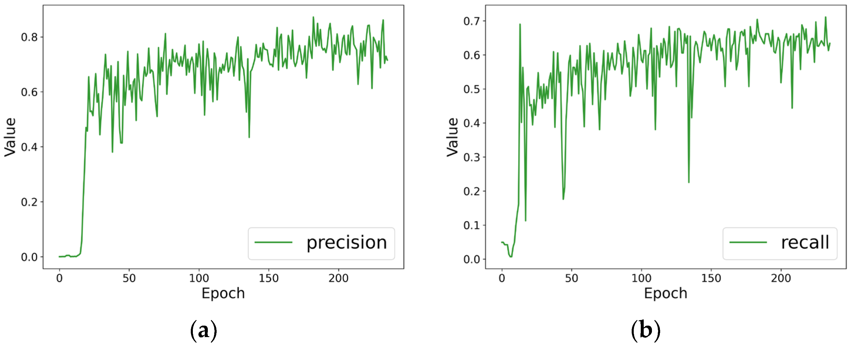
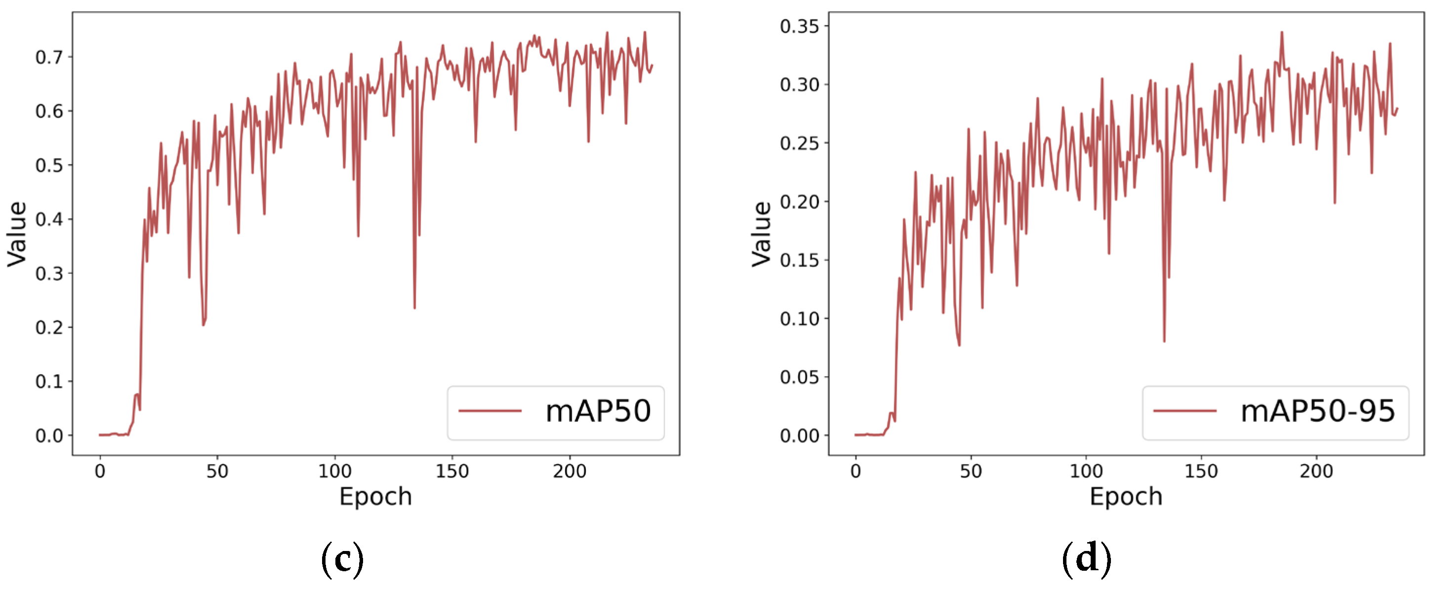
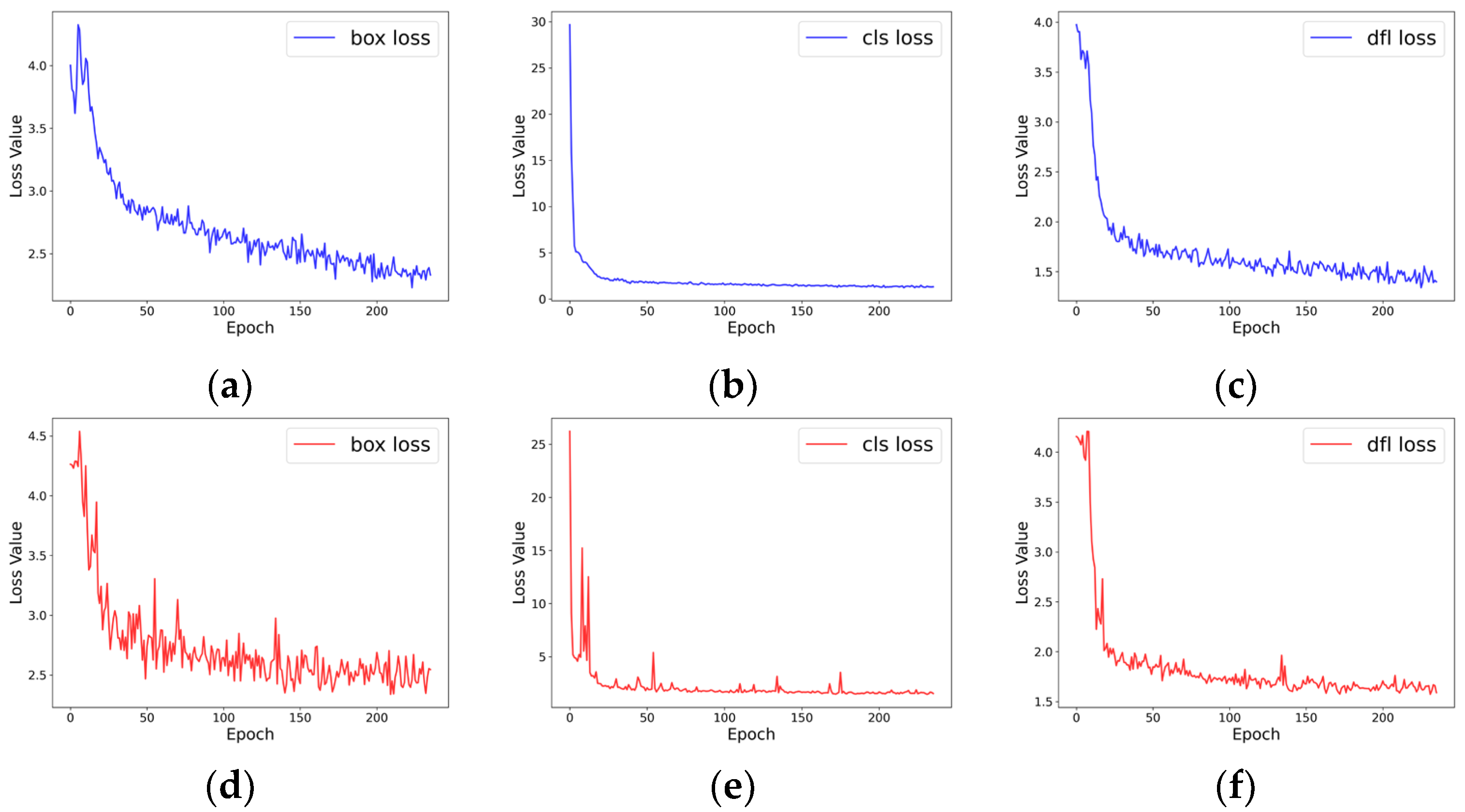
3.3.1. MF-YOLOv11 Model Checking Performance Evaluation

To evaluate the performance of the model, the following evaluation metrics were used in this experiment: accuracy, which reflects the proportion of actual positive samples among those predicted as positive; recall, which assesses the coverage of correctly identified true positive samples; mAP50, the mean average precision calculated at an IoU threshold of 0.5; and mAP50-95, the mean average precision calculated across IoU thresholds from 0.5 to 0.95, which comprehensively reflects the localization and classification ability for multi-class defect detection. The definitions of these evaluation metrics are given in Formulas (12) and (13). In the formula definition, TP stands for true positive, FP stands for false positive, FN stands for false negative, and TN stands for true negative.

$$Precision={\displaystyle \frac{TP}{TP+FP}}$$

(15)

$$Recall={\displaystyle \frac{TP}{TP+FN}}$$

(16)

The training of the MF-YOLOv11 model was conducted using the PyTorch v2.0.1 framework, with a batch size of 16 and a learning rate of 0.01, over a total of 250 epochs. The results of the training process are shown in Figure 7. As illustrated in Figure 7a, precision significantly improved after the 20th epoch and stabilized around the 150th epoch. Recall, presented in Figure 7b, also exhibited a notable increase after 20 epochs, continuing to rise steadily and stabilizing around the 150th epoch. The mAP50 and mAP50-95 metrics increased rapidly during the initial stages of training, followed by a noticeable dip around the 130th epoch, after which they continued to rise steadily and stabilized after approximately 200 epochs. These observations suggest that both precision and recall improved significantly early in the training process, indicating that the model quickly learned effective defect detection features, stabilizing after 150 epochs. As the training progressed, all metrics reached stability after around 200 epochs, indicating that the model had fully converged and that the training parameters were conducive to achieving consistent performance.

In addition to the model performance metrics mentioned above, the loss function used for optimizing the model is also of significant importance, as it reflects the degree of difference between the predicted results and the ground truth. The loss function includes bounding box regression loss, classification loss, and dynamic feature loss, with the specific results shown in Figure 8.

Figure 8a–c illustrate the training loss curves, reflecting the model’s fitting performance on the training data. Figure 8d–f depict the validation loss curves, assessing the model’s generalization ability on unseen data. Figure 8a shows the bounding box regression loss curve during training. After a brief increase in the early stages, the loss began to decrease and stabilized at around 200 epochs. Figure 8b illustrates the classification loss during training, which stabilized after 20 epochs and remained steady thereafter. Figure 8c depicts the dynamic feature loss during training, which decreased rapidly in the early stages, then slowed down after 30 epochs, and stabilized after 200 epochs. Figure 8d presents the bounding box regression loss on the validation set, which decreased rapidly in the early stages, then declined more gradually after 25 epochs, and stabilized after 150 epochs. The trend in the validation set aligns with that of the training set, indicating that the model’s generalization ability for localization tasks improved progressively and converged. Figure 8e illustrates the classification loss on the validation set, which stabilized after 20 epochs, with minor fluctuations afterward. Figure 8f depicts the dynamic feature loss on the validation set, which declined rapidly in the early stages and stabilized after 200 epochs, mirroring the trend observed in the training set. This indicates that the model’s performance on the validation set followed a similar trend to that of the training set, suggesting robust feature extraction capabilities on unseen data, with no significant indications of overfitting.

The optimal model achieved an accuracy of 86.1%, a recall rate of 71.1%, and an mAP50 of 72.7%. To visually assess the model’s detection performance, a subset of images was randomly selected from a validation set of 308 images, and the trained optimal model was applied for detection. The images in Figure 9a–c were captured without using polarization imaging. The yellow lines in these images highlight the curvature of the samples, simulating changes in complex surfaces by varying the curvature. Figure 9d–f display images obtained using polarization imaging, with defect detection results from the MF-YOLOv11 model. A visual comparison clearly demonstrates that polarization imaging effectively suppressed glare interference, preventing the loss of defect information and enhancing the overall uniformity of the imaging. It can be observed that the detection model accurately marked the defect locations, showcasing the model’s strong detection capability.

In addition to planar defects detected using polarization imaging, complex curved surfaces also contain numerous non-planar defects, which can be categorized into protruding defects and pit defects. Protruding defects are characterized by small defect scales, where the small targets occupy only a few pixels in the image, making it challenging for traditional convolutional neural networks to capture fine details. On the other hand, pit defects have larger defect scales but weaker semantic information, low contrast with the background, and more blurred boundaries. The proposed MF-YOLOv11 model, incorporating a multi-scale edge information selection module and an improved spatial pyramid pooling module, not only enhances the semantic information of defect edges but also adaptively fuses multi-scale features, improving the model’s detection capability for both types of defects. The specific detection results are as follows: Figure 10a–c show the detection labels for protrusion defects using the MF-YOLOv11 model, while Figure 11a–c show the detection labels for pit defects. The model demonstrated strong detection capabilities for both types of non-planar defects.

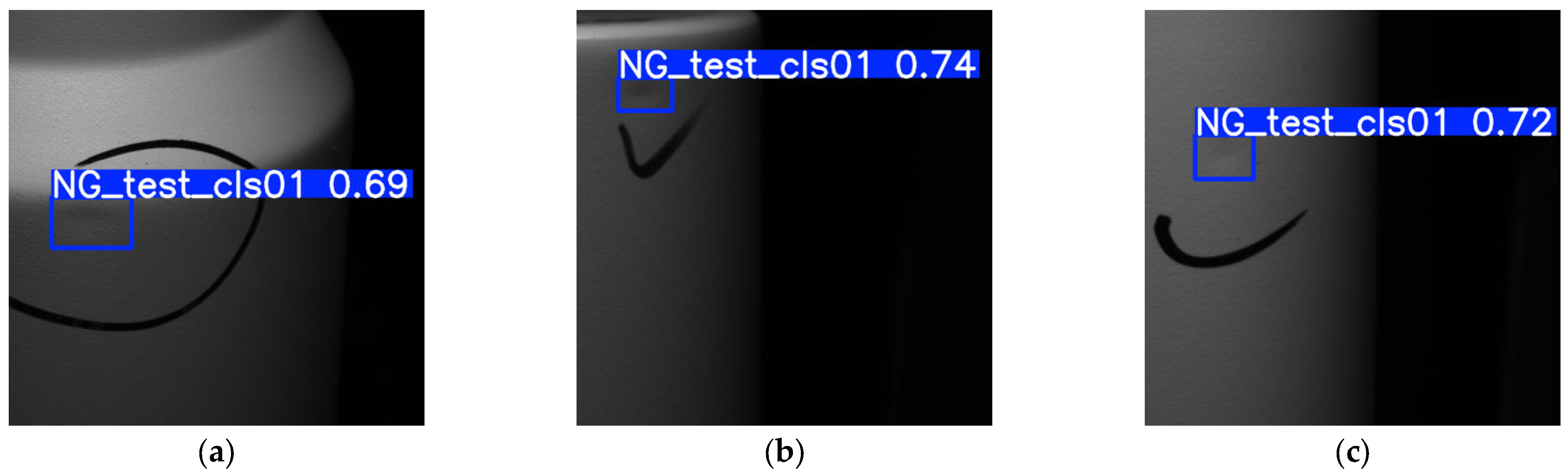
3.3.2. MF-YOLOv11 Model Detection Performance Comparison

From Figure 12, it can be seen that the detection accuracy of the Faster R-CNN model was relatively low, with a value of only 70.7%. Additionally, the FLOPs per inference were 17.9, indicating a high computational cost for inference. The improved network models based on DETR exhibited better detection performance. The RT-DETR model achieved a detection accuracy of 76.7%, and the Bearing-DETR model achieved 78.7%. However, both models required substantial computational resources, with a single inference time of around 2 s, which is not suitable for real-time defect detection. The CSGNet model is an improved version of the YOLOv6 model, offering a good balance between detection accuracy and computational speed. The Net-CA-SSD model, which uses ShuffleNetv2 as the backbone for the SSD detection framework, achieved a detection accuracy of 76.8%. However, like the improved DETR-based networks, it also suffered from longer inference times.

Compared to other models, the MF-YOLOv11n model demonstrates significant advantages, particularly in terms of both performance and efficiency. First, this model outperforms others in key detection metrics, with a precision of 86.1% and a recall of 71.1%, both of which are the highest values among all models. This indicates that it effectively reduces both false positives and false negatives. Its mAP50 score of 72.7% also surpasses that of other models, suggesting superior balance between bounding box localization accuracy and classification precision. This is crucial for high-precision detection requirements in industrial quality control. Secondly, the MF-YOLOv11n achieves a lightweight design while maintaining high performance. The model size is only 5.8 MB, significantly smaller than Faster-RCNN (27.4 MB) and RT-DETR (32.2 MB), and slightly smaller than the same series YOLOv11n (5.9 MB). Its FLOPs value is 7.6, which is relatively low, indicating that the model consumes fewer computational resources and is better suited for deployment on industrial devices or embedded systems with limited computational power. Compared to YOLOv10n and YOLOv11n, MF-YOLOv11n further enhances its ability to capture defect features by optimizing the network structure, making it better suited for adapting to the diverse defects present on complex surfaces. In conclusion, MF-YOLOv11 outperforms existing models in terms of higher detection accuracy, lower resource consumption, and stronger feasibility for industrial implementation.

3.3.3. Ablation Study

This study systematically conducted ablation experiments to verify the performance improvement of the MF-YOLOv11n model by incorporating the multi-scale edge information selection (MSIS) module and the Focal Modulation module. The experiments were performed on a self-constructed complex surface defect dataset, with key hyperparameters such as a fixed batch size of 16 and an initial learning rate of 0.01 to minimize the influence of extraneous variables. The baseline model used was the original YOLOv11n architecture. Comparative experiments were conducted by replacing the C3k2 module in the neck with the C3k2-MSIS module and substituting the SPPF module in the backbone with the Focal Modulation module. The YOLOv11n model with only the C3k2-MSIS module replacement was designated as YOLOv11n-C3k2-MSIS, while the model with only the Focal Modulation module replacement was named YOLOv11n-Focal Modulation. The experimental results are summarized in

Table 3. Ablation experiment results.

Model Name	Precision	Recall	mAP50	Model Size	GFLOPS
YOLOv11n	82.2	68.3	71.1	5.9	7.3
YOLOv11n-C3k2-MSIS	83.7	69.2	71.6	5.8	7.4
YOLOv11n-Focal Modulation	84.3	69.7	71.8	5.8	7.4
MF-YOLOv11n	86.1	71.1	72.7	5.8	7.6

.

It can be observed that, compared to the YOLOv11n baseline model, the introduction of the C3k2-MSIS module improved the model’s accuracy by 1.5%, reaching 83.7%, recall by 0.9%, reaching 69.2%, and mAP50 by 0.5%, reaching 71.6%. On the other hand, the model with the Focal Modulation module showed more significant improvements, with accuracy increasing by 2.1% to 84.3%, recall increasing by 1.4% to 69.7%, and mAP50 increasing by 0.7% to 71.8%. When both improvement strategies were integrated into MF-YOLOv11n, the model achieved the best overall performance while maintaining a model complexity similar to that of the baseline model. This indicates that the two modules complement each other in enhancing edge feature extraction and dynamically focusing on key areas, effectively balancing detection accuracy and computational efficiency.

4. Conclusions

This study addresses the challenge of defect detection on the surfaces of industrial components with complex curvatures by proposing a combined approach that integrates a polarization imaging system with an improved MF-YOLOv11 model. The polarization imaging system employs a curved light source specifically designed to adapt to complex surfaces, ensuring uniform illumination. Additionally, a polarization imaging unit is constructed, where horizontal and vertical polarizers work in tandem to capture images in a single exposure while effectively suppressing glare interference. The polarization imaging method outperforms other approaches across all evaluation metrics. The MF-YOLOv11 model incorporates a multi-scale edge information selection module and a Focal Modulation module. The multi-scale edge information selection module employs adaptive pooling and parallel convolutional branches to process features at different scales, utilizing an edge enhancement module to enhance edge information and achieve multi-scale feature fusion. The Focal Modulation module applies hierarchical convolution to extract multi-scale contextual information and integrates a dynamic gating mechanism for feature aggregation. These module enhancements significantly improve the model’s ability to detect defects of various forms on complex surfaces. Experimental results demonstrate that, on the self-constructed dataset, the MF-YOLOv11 model achieved a precision of 86.1%, reflecting a 3.9% improvement over the baseline YOLOv11n model. The recall reached 71.1%, an increase of 2.8% over the baseline, while the mAP50 metric achieved 72.7%, improving by 1.6%. Furthermore, the inference time per sample was less than 35 ms, meeting the real-time requirements for industrial defect detection.

References

1. Zarei, A.; Pilla, S. Laser ultrasonics for nondestructive testing of composite materials and structures: A review. Ultrasonics 2024, 136, 107163. [Google Scholar] [CrossRef] [PubMed]
2. Li, E.; Guo, W.; Cao, X.; Zhu, J. A magnetic head-based eddy current array for defect detection in ferromagnetic steels. Sens. Actuators A Phys. 2024, 379, 115862. [Google Scholar] [CrossRef]
3. Chang, H.-L.; Ren, H.-T.; Wang, G.; Yang, M.; Zhu, X.-Y. Infrared defect recognition technology for composite materials. Front. Phys. 2023, 11, 1203762. [Google Scholar] [CrossRef]
4. Ren, Z.; Fang, F.; Yan, N.; Wu, Y. State of the Art in Defect Detection Based on Machine Vision. Int. J. Precis. Eng. Manuf.-Green Technol. 2021, 9, 661–691. [Google Scholar] [CrossRef]
5. Wen, X.; Shan, J.; He, Y.; Song, K. Steel Surface Defect Recognition: A Survey. Coatings 2022, 13, 17. [Google Scholar] [CrossRef]
6. Kim, T.; Behdinan, K. Advances in machine learning and deep learning applications towards wafer map defect recognition and classification: A review. J. Intell. Manuf. 2022, 34, 3215–3247. [Google Scholar] [CrossRef]
7. Xie, Y.; Xu, X.; Liu, S. Machine vision-based detection of surface defects in cylindrical battery cases. J. Energy Storage 2024, 101, 113949. [Google Scholar] [CrossRef]
8. Qiao, J.; Sun, C.; Cheng, X.; Yang, J.; Chen, N. Stainless steel cylindrical pot outer surface defect detection method based on cascade neural network. Meas. Sci. Technol. 2023, 35, 036201. [Google Scholar] [CrossRef]
9. Abdulrahman, Y.; Mohammed Eltoum, M.A.; Ayyad, A.; Moyo, B.; Zweiri, Y. Aero-engine Blade Defect Detection: A Systematic Review of Deep Learning Models. IEEE Access 2023, 11, 53048–53061. [Google Scholar] [CrossRef]
10. Jing, J.; Liu, S.; Wang, G.; Zhang, W.; Sun, C. Recent advances on image edge detection: A comprehensive review. Neurocomputing 2022, 503, 259–271. [Google Scholar] [CrossRef]
11. Tsai, D.-M.; Huang, C.-K. Defect Detection in Electronic Surfaces Using Template-Based Fourier Image Reconstruction. IEEE Trans. Compon. Packag. Manuf. Technol. 2019, 9, 163–172. [Google Scholar] [CrossRef]
12. Li, F.; Yuan, L.; Zhang, K.; Li, W. A defect detection method for unpatterned fabric based on multidirectional binary patterns and the gray-level co-occurrence matrix. Text. Res. J. 2019, 90, 776–796. [Google Scholar] [CrossRef]
13. Sahu, D.; Dewangan, R.K.; Matharu, S.P.S. An Investigation of Fault Detection Techniques in Rolling Element Bearing. J. Vib. Eng. Technol. 2023, 12, 5585–5608. [Google Scholar] [CrossRef]
14. Dong, G.; Pan, X.; Liu, S.; Wu, N.; Kong, X.; Huang, P.; Wang, Z. A review of machine vision technology for defect detection in curved ceramic materials. Nondestruct. Test. Eval. 2024, 1–27. [Google Scholar] [CrossRef]
15. Zhou, A.; Ai, B.; Qu, P.; Shao, W. Defect detection for highly reflective rotary surfaces: An overview. Meas. Sci. Technol. 2021, 32, 062001. [Google Scholar] [CrossRef]
16. Xu, L.M.; Yang, Z.Q.; Jiang, Z.H.; Chen, Y. Light source optimization for automatic visual inspection of piston surface defects. Int. J. Adv. Manuf. Technol. 2016, 91, 2245–2256. [Google Scholar] [CrossRef]
17. Shao, W.; Liu, K.; Shao, Y.; Zhou, A. Smooth Surface Visual Imaging Method for Eliminating High Reflection Disturbance. Sensors 2019, 19, 4953. [Google Scholar] [CrossRef]
18. Hui, M.; Li, M.; Babar, M. A Diffuse Reflection Approach for Detection of Surface Defect Using Machine Learning. Mob. Inf. Syst. 2022, 2022, 7771178. [Google Scholar] [CrossRef]
19. Chen, H.; Gao, J.; Zhang, Z.; Yin, W.; Dong, N.; Zhou, G.; Meng, Z. CFRP delamination defect detection by dynamic scanning thermography based on infrared feature reconstruction. Opt. Lasers Eng. 2025, 187, 108884. [Google Scholar] [CrossRef]
20. Bao, Y.; Zhou, Z.; Wei, S.; Xiang, J. Research on surface defect detection system and method of train bearing cylindrical roller based on surface scanning. J. Mech. Sci. Technol. 2023, 37, 4507–4519. [Google Scholar] [CrossRef]
21. Wang, D.; Yin, J.; Wu, H.; Ge, B. Method for detecting internal cracks in joints of composite metal materials based on dual-channel feature fusion. Opt. Laser Technol. 2023, 162, 109263. [Google Scholar] [CrossRef]
22. Zheng, X.; Liu, W.; Huang, Y. A Novel Feature Extraction Method Based on Legendre Multi-Wavelet Transform and Auto-Encoder for Steel Surface Defect Classification. IEEE Access 2024, 12, 5092–5102. [Google Scholar] [CrossRef]
23. Liu, Z.; Qu, B. Machine vision based online detection of PCB defect. Microprocess. Microsyst. 2021, 82, 103807. [Google Scholar] [CrossRef]
24. Hussain, M. YOLO-v1 to YOLO-v8, the Rise of YOLO and Its Complementary Nature toward Digital Manufacturing and Industrial Defect Detection. Machines 2023, 11, 677. [Google Scholar] [CrossRef]
25. Ren, S.; He, K.; Girshick, R.; Sun, J. Faster R-CNN: Towards Real-Time Object Detection with Region Proposal Networks. IEEE Trans. Pattern Anal. Mach. Intell. 2017, 39, 1137–1149. [Google Scholar] [CrossRef]
26. Ameri, R.; Hsu, C.-C.; Band, S.S. A systematic review of deep learning approaches for surface defect detection in industrial applications. Eng. Appl. Artif. Intell. 2024, 130, 107717. [Google Scholar] [CrossRef]
27. Song, K.; Sun, X.; Ma, S.; Yan, Y. Surface Defect Detection of Aeroengine Blades Based on Cross-Layer Semantic Guidance. IEEE Trans. Instrum. Meas. 2023, 72, 1–11. [Google Scholar] [CrossRef]
28. Zhao, H.; Gao, Y.; Deng, W. Defect Detection Using Shuffle Net-CA-SSD Lightweight Network for Turbine Blades in IoT. IEEE Internet Things J. 2024, 11, 32804–32812. [Google Scholar] [CrossRef]
29. Li, D.; Li, Y.; Xie, Q.; Wu, Y.; Yu, Z.; Wang, J. Tiny Defect Detection in High-Resolution Aero-Engine Blade Images via a Coarse-to-Fine Framework. IEEE Trans. Instrum. Meas. 2021, 70, 1–12. [Google Scholar] [CrossRef]
30. Liu, M.; Wang, H.; Du, L.; Ji, F.; Zhang, M. Bearing-DETR: A Lightweight Deep Learning Model for Bearing Defect Detection Based on RT-DETR. Sensors 2024, 24, 4262. [Google Scholar] [CrossRef]
31. Chang, F.; Liu, M.; Dong, M.; Duan, Y. A mobile vision inspection system for tiny defect detection on smooth car-body surfaces based on deep ensemble learning. Meas. Sci. Technol. 2019, 30, 125905. [Google Scholar] [CrossRef]
Figure 1. Polarization imaging system principle.
Photonics 12 00368 g001
Figure 2. MF-YOLOv11 network architecture.
Photonics 12 00368 g002
Figure 3. Multi-scale edge information selection module framework. a and b are learnable weights designed to enable adaptive adjustment of channel features. In the diagram, a indicates that the feature is multiplied by weight a during this process, while b denotes multiplication by weight b.
Photonics 12 00368 g003
Figure 4. Gating mechanism principle.
Photonics 12 00368 g004
Figure 5. Photographs of experimental equipment. (a) Fixing module. (b) Servo motor. (c) Polarization camera. (d) Side camera. (e) Ring light.
Photonics 12 00368 g005
Figure 6. Image quality evaluation indicators. (a) RMS noise; (b) standard deviation; (c) uniformity index.
Photonics 12 00368 g006
Figure 7. Training evaluation metrics. (a) Precision; (b) recall; (c) mAP50; (d) mAP50-95.
Photonics 12 00368 g007aPhotonics 12 00368 g007b
Figure 8. Model loss function. (a) Training set box loss; (b) training set classification loss; (c) training set distribution focal loss (DFL); (d) validation set box loss; (e) validation set classification loss; (f) validation set distribution focal loss (DFL).
Photonics 12 00368 g008
Figure 9. Detection effect of plane defects. (a) Sample 1 without polarization imaging; (b) Sample 2 without polarization imaging; (c) Sample 3 without polarization imaging; (d) Sample 1 with polarization imaging; (e) Sample 2 with polarization imaging; (f) Sample 3 with polarization imaging.
Photonics 12 00368 g009
Figure 10. Detection effect of protrusion defects. (a) Detection result of Sample 1; (b) Detection result of Sample 2; (c) Detection result of Sample 3.
Photonics 12 00368 g010
Figure 11. Detection effect of pit defects. (a) Detection result of Sample 1; (b) Detection result of Sample 2; (c) Detection result of Sample 3.
Photonics 12 00368 g011
Figure 12. Model performance comparison. (a) Faster R-CNN; (b) RT-DETR; (c) Bearing-DETR; (d) CSGNet; (e) Net-CA-SSD; (f) YOLOV3n; (g) YOLOV5n; (h) YOLOV8n; (i) YOLOv9n; (j) YOLOV10n; (k) YOLOV11n; (l) MF-YOLOv11n.
Photonics 12 00368 g012