Vibration Deformation Measurement and Defect Identification Based on Time-Averaged Digital Holography

Abstract

Based on time-averaged digital holography, a vibration deformation measurement system was designed and a full process reconstruction and identification strategy was developed for detecting the micro-defects in optical materials. Through the double beam expansion setting and off-axis imaging adjustments, it is suitable for measuring optical materials with non-specular surfaces by double exposure shots. The scheme was applied to optical sandwich composites and 3D printed glass. Abnormal amplitudes occur at the defects due to different resonance frequencies, resulting in anomalous vibrations under excitation, and the differences in the amplitudes and phases before and after vibration can effectively characterize vibration amplitude and subsurface defects, proving that this method has a high detecting sensitivity.

1. Introduction

Defects in optical materials, often caused by improper fabrication, transportation, and applications, can significantly impact the performance and reliability of optical functional components. As a result, sensitive and efficient detection methods of the micro-defects are urgently required. However, existing non-destructive testing methods suffer from long scanning times, high equipment costs, and limited applicability, and it is especially challenging to detect subsurface defects which are not visible from the surface topography. This paper proposes a digital holographic microscopy approach combined with vibration fields to achieve highly sensitive defect identification on rough optical surfaces.

Digital holography enables real-time and dynamic object detection and 3D imaging through numerical computation. It has been widely used in vibration measurement [1,2,3,4,5,6]. In the 1960s, Powell et al. introduced time-averaged holography, a technique for non-contact, non-destructive testing of stress-, vibration-, and heat-induced deformations [7]. With the development of information technology, in 2003, Picart et al. [8] extended time-averaged holography to digital holography, which captures images by CMOS or CCD sensors instead of recording holographic films. In 2007, Anand Asundi et al. [9] of Nanyang Technological University successfully applied double exposure time-averaged online digital holography to the dynamic characterization of MEMS films. In 2014, Bruno et al. [10] proposed a real-time, wide-field structural detection method to identify delamination defects in sandwich composite panels.

In 2012, Psota et al. [11] introduced a phase shifting heterodyne digital holography method to directly obtain the absolute vibration amplitude at the nanometer and sub-nanometer scales. They later proposed scanning time-averaged holography in 2018 [12], allowing for independent pixel-wise vibration measurements via phase modulation of either the reference or object wave. In 2019, they further optimized phase modulation to measure vibrations in high-slope and partially occluded regions [13]. In 2024, Fu et al. [14] proposed a method to characterize nano/micro membrane resonators by analyzing the average interference fringes obtained by continuous light measurements.

In order to solve the problem of mutual interference between the zero-order term and the conjugate term in the holographic image [15], generally, the positive first-order term in the spectrum domain is extracted, and then, an inverse transform is performed to obtain the complex amplitude [16,17,18,19,20]. In off-axis digital holography, these three terms can be completely separated by adjusting the off-axis angle, allowing for double exposure-shot detection of dynamic scenarios. However, speckles occur when the detecting light is reflected from or transmitted through rough surfaces, which significantly degrade the holographic image quality, prompting recent research on speckle denoising techniques. In 2020, Yan et al. [21] proposed a CNN-based phase denoising method. In 2021, Wang et al. [22] introduced an image denoising approach combining the sine–cosine transform with BM3D, while Xiao et al. [23] developed a phase denoising technique based on empirical wavelet transform and cross-correlation. Later, in 2022, Niu et al. [24] proposed a windowed Fourier filtering method. Most recently, in 2024, Chen et al. [25] introduced a Swin-UNet-based speckle denoising technique.

Vibration measurement methods based on digital holography commonly employ time-averaging techniques to capture interference fringes, enabling quantitative deformation analysis through fringe analysis and numerical computation. Since coaxial holography phase-shifting techniques are unsuitable for dynamic detection, this study adopts off-axis digital holography for vibration measurement and defect detection.

2. Theoretical Basis of Vibration Deformation Measurement

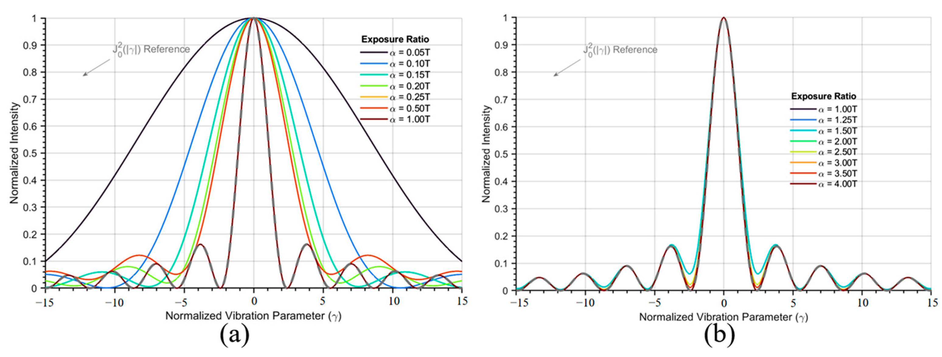
2.1. Principle of Time-Averaged Digital Holography

When the exposure time of a CMOS camera far exceeds the vibration period of a vibrating object, the hologram can record the motion state of multiple vibration periods. This type of hologram is called a time-averaged hologram.

Assume that the out-of-plane displacement of an object vibrating sinusoidally is as follows:

$$\overrightarrow{z}(x,y,t)=\overrightarrow{z_0}(x,y)+{\overrightarrow{z}}_v(x,y)\sin \omega t$$

(1)

where $\omega$ is the angular frequency of vibration, $\overrightarrow{z_0}(x,y)$ is the average deformation displacement, and $\overrightarrow{z_v}(x,y)$ is the time-varying displacement [9]. The instantaneous object wave scattered from the vibrating object is as follows:

$$O(x,y,t)=O_0(x,y)\exp \left\{i\left[\overrightarrow{K}\cdot \overrightarrow{z}(x,y,t)\right]\right\}$$

(2)

where $O_0(x,y)$ is the complex amplitude of the scattered light when the object is stationary, and $\overrightarrow{K}$ is the sensitivity vector.

Such a time-averaged hologram is actually the integration of the light intensity during the image acquisition period, and the resulting object wave is as follows [9]:

$$\begin{array}{ll}O(x,y)& ={\displaystyle \frac{1}{\tau }}{\displaystyle {\int }_0^{\tau }O(x,y,t)d\tau }\\ & =O_0(x,y)\exp \left\{i\varphi (x,y)\right\}\times J_0\left\{\overrightarrow{K}\cdot \overrightarrow{z_v}(x,y)\right\}\end{array}$$

(3)

where $J_0$ is the zero-order Bessel function, and $\varphi (x,y)$ is the phase of the target wave, which contains the information of the average static phase and the zero point of the Bessel function [26]

$$\varphi (x,y,t)={\varphi }_0(x,y)+{\varphi }_J(x,y,t)={\varphi }_0(x,y)+{\displaystyle \frac{4\pi }{\lambda }}d(x,y)\sin (\omega t)$$

(4)

where ${\varphi }_0(x,y)$ denotes the phase map of the object wave, which can be considered as the speckle noise source in the case of pure time-averaging. ${\varphi }_J(x,y,t)$ is the time-average phase, $\lambda$ is the wavelength of the imaging light, and $d(x,y)$ is the vibration amplitude.

Using the integral definition of the Bessel function, the intensity of the reconstructed image is proportional to the square of the zero-order Bessel function [26], that is, $I_{rec}\propto J_0^2\left[4\pi d/\lambda \right]$. The fringe pattern of the target image is modulated by the square of the zero-order Bessel function. The nodes of the vibrating object correspond to the maxima and are, therefore, brighter in the holographic interferogram, while the dark fringes correspond to the zeros of the function $J_0^2$. These fringes can be used to locate regions of different vibration amplitudes [27].

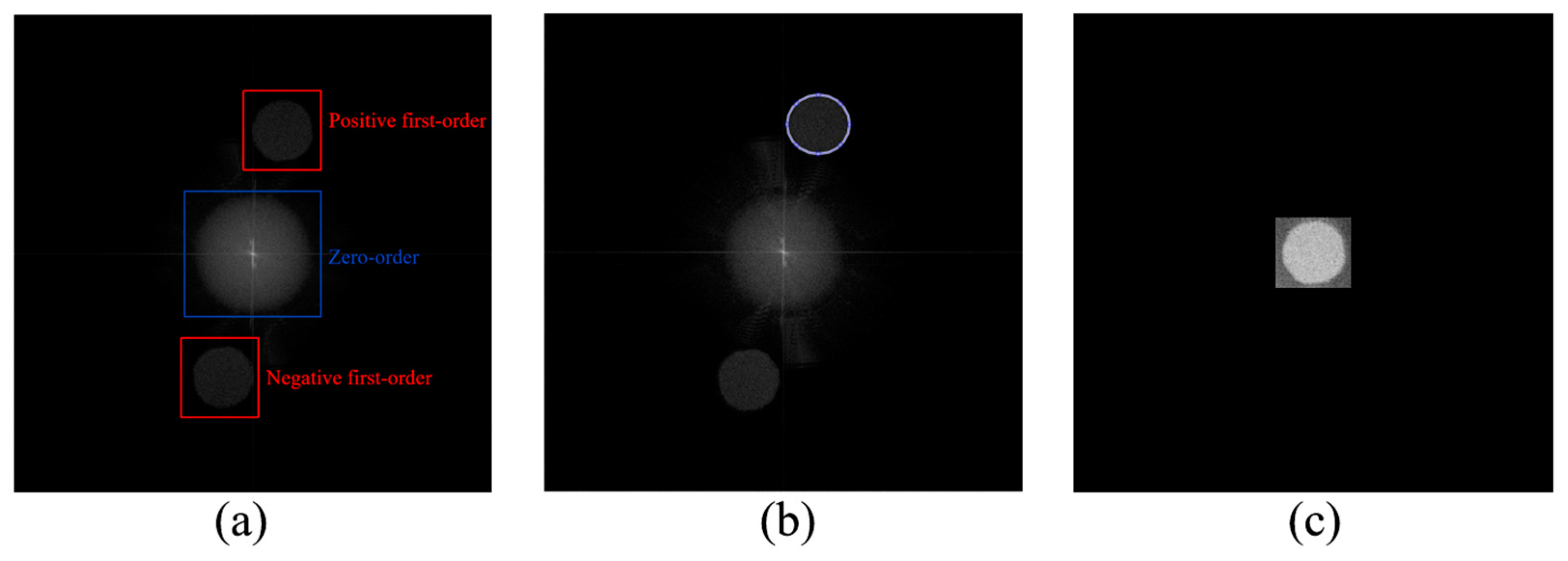
2.2. Phase Retrieval

Assuming that an object under test vibrates sinusoidally with two different amplitudes $z_1$ and $z_2$ at an angular frequency $\omega$, if the two vibration states are recorded by the time-averaged digital holography method, the associated complex amplitudes $U_1$ and $U_2$ can be obtained by numerical reconstruction. In order to eliminate the background and twin terms, the double exposure method is used for wave field subtraction as follows:

$$U_1-U_2=O_0(x^{\prime },y^{\prime })\left\{e^{i{\varphi }_1(x^{\prime },y^{\prime })}\times J_0\left[\overrightarrow{K}\cdot {\overrightarrow{z}}_1(x^{\prime },y^{\prime })\right]-e^{i{\varphi }_2(x^{\prime },y^{\prime })}\times J_0\left[\overrightarrow{K}\cdot {\overrightarrow{z}}_2(x^{\prime },y^{\prime })\right]\right\}$$

(5)

The intensity subtraction of the double exposure method contains mixed fringes, including average static deformation fringes and zero-order Bessel fringes. The difference in amplitude corresponds to the Bessel-type vibration fringes, while the difference in phase corresponds to the average deformation as ${\cos }^2$ fringes. In order to extract the vibration deformation information, the Bessel fringes need to be separated [28].

To minimize spectrum aliasing in speckle interference, the holograms before and after vibration are first interpolated in advance, using the Kronecker product of a 3 × 3 unit matrix [29]. After suppressing the zero-order term, the positive first-order term is extracted via spectrum filtering to enhance the reconstructed image quality. As shown in Figure 1a, adjusting the angle between the object and reference light allows complete separation of the zero-order and first-order spectral terms, as indicated using a red and blue box, respectively. Given that the zero-order term corresponds to low frequencies while the positive first-order term carries interference information at higher frequencies, bandpass filtering is applied to fully extract the interference signal. Figure 1b illustrates the extracted positive first-order term, and Figure 1c demonstrates carrier elimination by centering the high-frequency component in the spectrum.

After the positive first-order term is extracted and placed at the center of the spectrum domain, the wrapped phase can be obtained by inverse Fourier transforms. However, there is a large amount of speckle noise, which will affect the accuracy of subsequent phase measurement [30,31].

Commonly used spatial denoising methods include mean and median filtering, which operate on the image by sliding a window and adjusting the window size according to the actual image being processed. However, when the window is moved, the noise will be dispersed, resulting in the loss of phase mutation information. The sine and cosine phase images are obtained by the sine and cosine transform method and then subjected to denoising, respectively. This method can not only improve the denoising effect but also retain the phase jump information [22]. Let $g_0(x,y)$ be the image to be processed, $g_1(x,y)$ and $g_2(x,y)$ be the image after sine and cosine transforms, respectively.

$$\begin{array}{l}{g}_1(x,y)=\left[1+\sin {\displaystyle \frac{g_0(x,y)\times 2\pi }{255}}\right]\times {\displaystyle \frac{255}{2}}\\ g_2(x,y)=\left[1+\cos {\displaystyle \frac{g_0(x,y)\times 2\pi }{255}}\right]\times {\displaystyle \frac{255}{2}}\end{array}$$

(6)

The images obtained by the sine and cosine transforms are subjected to BM3D filtering [22], and then the denoised results are subjected to the arctangent operation ${\overline{g}}_0(x,y)=\arctan \left[{\overline{g}}_1(x,y)/{\overline{g}}_2(x,y)\right]$ to obtain a phase map with a good denoising effect. While among those transform-based methods, wavelet denoising decomposes the signal into components of different scales through wavelet transforms and removes noise by setting thresholds; the window Fourier method performs local filtering in the frequency domain by setting a Gaussian window [24].

When calculating the phase difference before and after vibration in the subsequent step, the sine and cosine transform combined with the BM3D method is adopted for denoising because of its superior flexibility and adaptability.

3. Analysis of Impacts of Configuration Parameters

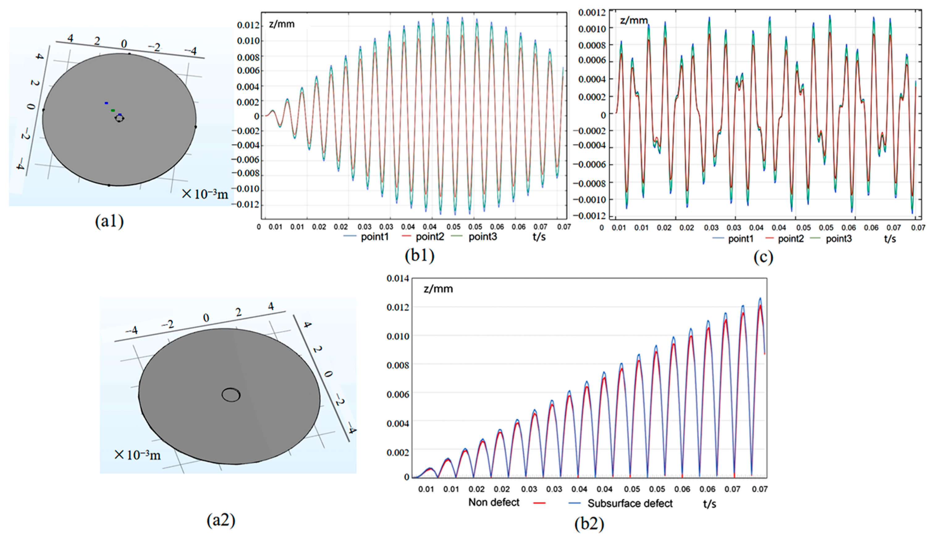
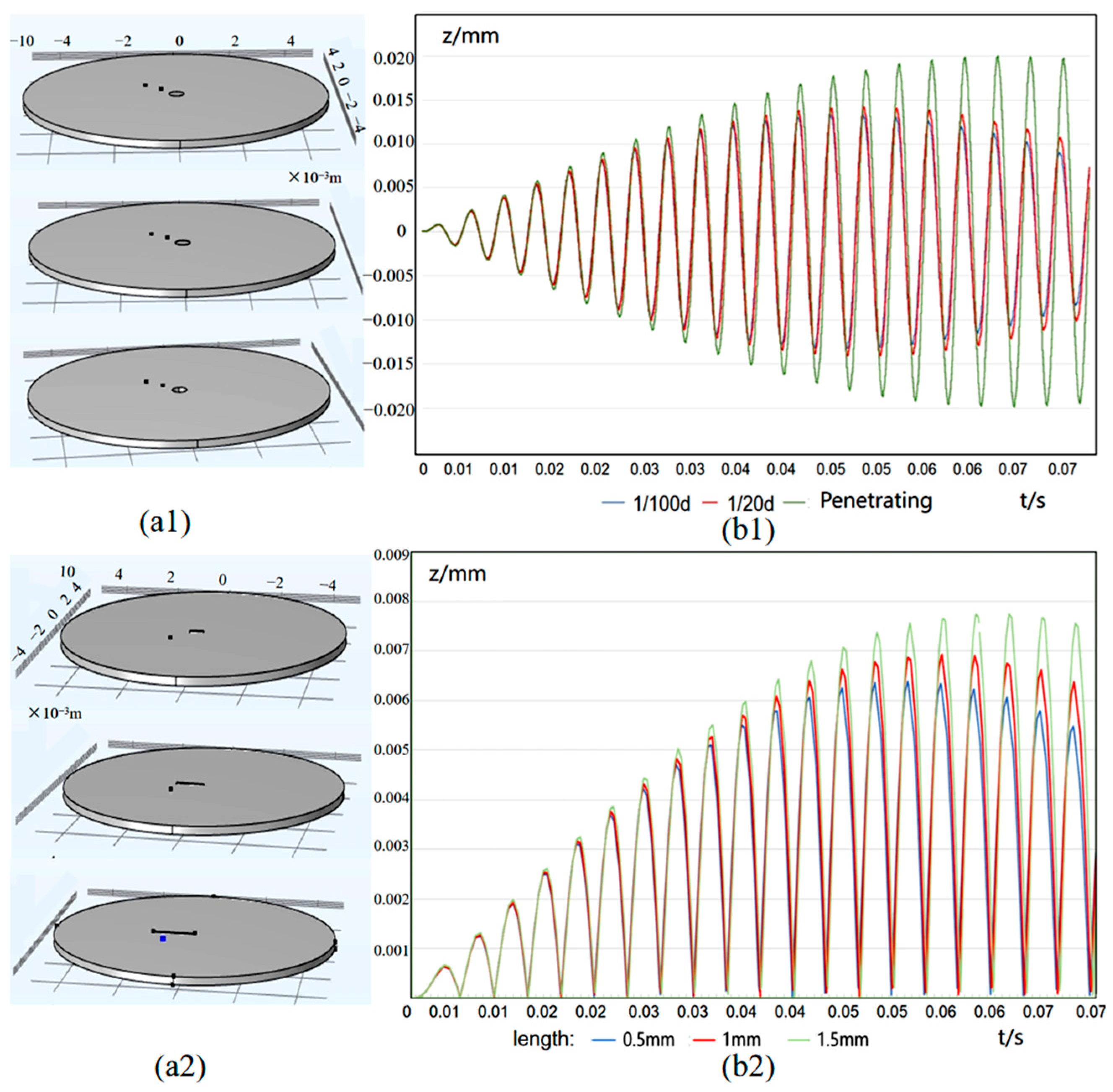
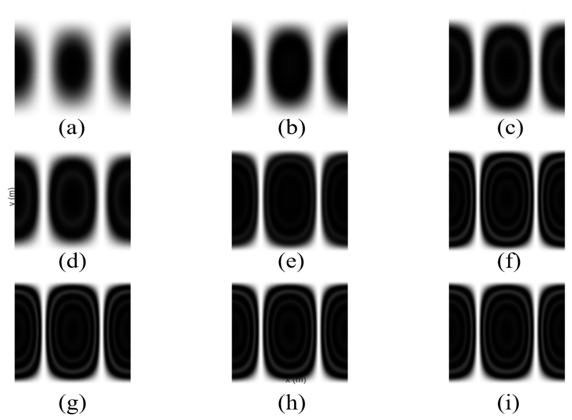
3.1. Simulation of Stimulated Vibration of Objects

When an object is subjected to external excitation, its surface undergoes vibration and, consequently, deformation displacement. The loudspeaker employed generates a sinusoidal excitation signal and the vibrating amplitude can be modulated by a Bessel function. Defects reduce the local stiffness of material under test, thereby altering its local resonance frequency. When the excitation frequency approaches the resonance frequency of the defect region, significant amplitude amplification occurs. Simultaneously, local stress concentration at the defect site induces vibration energy dissipation, leading to anomalous amplitude behavior. To investigate the effect of defects on vibration amplitude and simplify parameter settings, this study employs COMSOL 6.1 for the finite element simulation of a simplified, circular, thin plate subjected to sinusoidal excitation.

First, a 3D structure, solid mechanics module, and transient solver are selected in COMSOL to model a cylindrical geometry with a diameter of 10 mm and a thickness of 0.2 mm. In order to study the effect of defects, geometries with different types of defects are also set. The material is set to PDMS in batches, and the material properties in the linear elastic material settings are defined.

Next, the physical field parameters are configured. The cylindrical sidewalls are fixed as constraints, while the front surface is designated as the boundary load region, where a sinusoidal excitation is applied. Previous studies have shown that the resonant frequency of thin plates of the same size is about 100–200 Hz. Under the resonant frequency excitation, the material surface will show a larger vibration amplitude. Therefore, the excitation frequency $f_0$ is set to the estimated resonant frequency of 140 Hz. The load expression is $F=A\sin \left(2\pi f_{0}t\right)$, where A is the amplitude.

Subsequently, a free tetrahedral mesh is used to segment the 3D structure, with finer meshing around the defect regions. Finally, in the transient solver, the time step is selected as $0.01/f_0$, and the duration time as $20/f_0$.

As shown in Figure 2(a1), a geometric model with a circular hole defect is constructed, where the depth of the hole defect was set to 1/100 of the thickness of the circular plate. A numerical solution was performed on this geometric structure, and three coordinate points were selected to calculate the difference of the displacement over time, as shown in Figure 2(b1). The closer to the defect area, the greater the vibration amplitude, which is consistent with theoretical analysis; thus, the amplitude at the defect can be used as an important indicator for defect identification. At resonance, the amplitude closely follows the excitation waveform; however, since the precise resonance frequency of the material is difficult to determine, an excitation frequency of 80 Hz is used. The displacement variation at non-resonant conditions in Figure 2c still shows significant amplitude differences between the defect and surrounding areas.

Subsequent simulations still maintain the excitation frequency at 140 Hz. In order to explore the influence of non-surface defects on surface vibration deformation, a cylinder with a radius of 0.5 mm is added to the back side. The cylinder does not penetrate the surface. A new model is obtained by subtracting the original geometric model and the cylinder through the Boolean operation as shown in Figure 2(a2). Subsequently, the multi-cycle amplitude difference with and without subsurface defects is obtained, and the amplitude difference is plotted in Figure 2(b2). The results show that subsurface defects will affect the displacement field and increase the vibrating amplitude in the defective area, thus proving that subsurface defects can be effectively identified according to the amplitude anomality.

In order to study the influence of defect size on the surface vibration, circular hole defects of different depths are set in the model, which are d/100, d/20, and d, respectively, with d denoting the plate thickness, as shown in Figure 3(a1). A specific measurement point around the defect is set to analyze the numerical difference of the displacement field changing with time under different circular hole defect conditions, as shown in Figure 3(b1). In addition, crack defects of different lengths, namely 0.5 mm, 1 mm, and 1.5 mm, are set, as shown in Figure 3(a2). The same measurement point is selected to analyze the numerical difference of the displacement field changing with time under different crack defect conditions, as shown in Figure 3(b2).

As can be seen from Figure 3(b1), with the increase in the circular hole depth, the vibration amplitude of the measurement points around the defect gradually increases, especially when the circular hole defect penetrates the plate surface, and the amplitude value increases significantly. This may be because the presence of the circular hole defect reduces the local rigidity of the circular plate, resulting in the amplification of the amplitude. As can be seen from Figure 3(b2), with the increase in the crack length, the displacement field value of the point near the crack also gradually increases. This shows that the crack size has a significant effect on the vibration field. Based on the above numerical simulation results, effective distinction of defect sizes can be achieved.

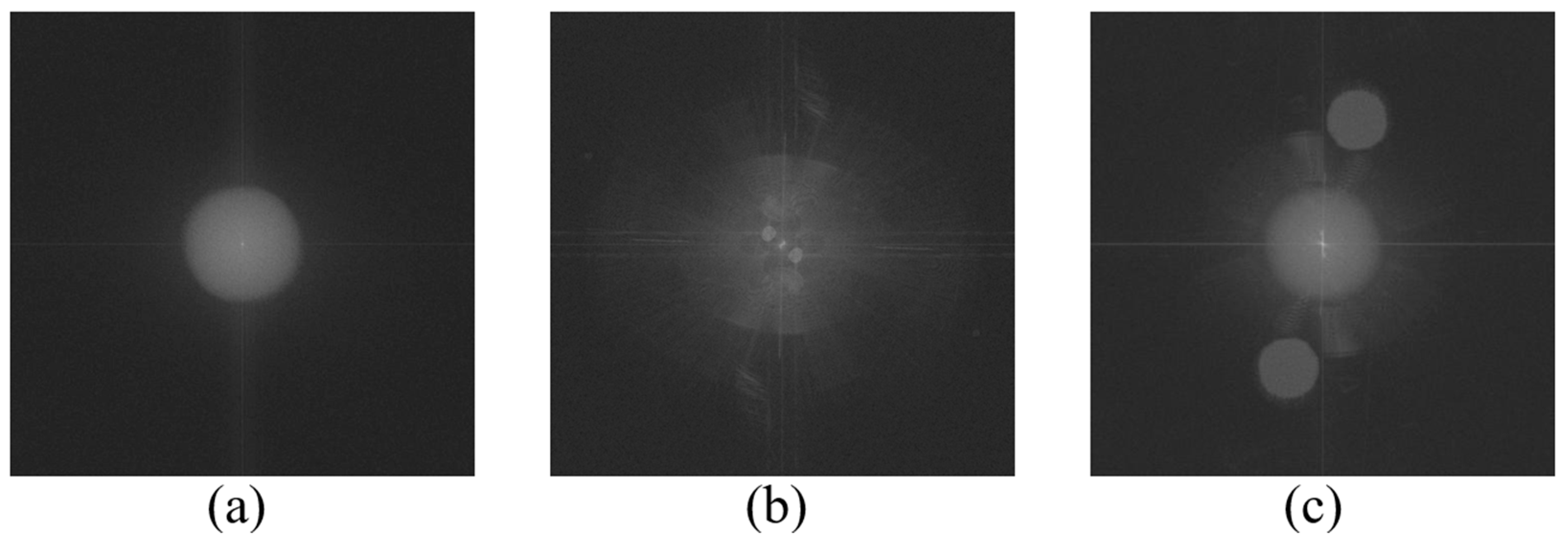
3.2. Hologram Recording

When the vibration period is much smaller than the exposure time, the envelope of the Bessel function $J_0$ appears in the integrated image of the object light wave. Luis et al. proposed that the amplitude result is affected by the exposure time and can be expressed as follows [27]:

$$E\left(\gamma ,\alpha \right)=\left|J_0(\gamma )\alpha +{\displaystyle \sum _{m=1}^{\infty }\frac{J_{2m}(\gamma )}{m}\sin (2m\alpha )+2i{\displaystyle \sum _m^{\infty }\frac{J_{2m-1}(\gamma )}{2m-1}\left(1-\cos \left(\left(2m-1\right)\alpha \right)\right)}}\right|$$

(7)

Among them, $\gamma$ is the vibration amplitude, $\alpha$ is the exposure time, m is the number of Bessel series truncated terms, and $J_0\left(\gamma \right)$ is the zero-order Bessel function.

The amplitude envelopes associated with different exposure times $\alpha$ are shown in Figure 4. It can be seen that the envelope gradually approaches $J_0$ as the exposure time gradually increases from a very short time to a time equal to the vibration period. When the exposure time is relatively shorter than the vibration period, the high-order Bessel function has a significant impact. When the exposure time is equal to the vibration period, the Bessel envelope is still valid. On the contrary, when the exposure time continues to increase, the distribution of light and dark rings in the reconstructed image is completely determined by $J_0$.

In order to verify the influence of changing the exposure time, the fundamental frequency vibration of a circular film with the edge fixed is simulated, the complex amplitude envelope is calculated, and the series truncation is set to 20 terms to ensure that high-order Bessel terms can be ignored, as shown in Figure 5. It can be seen that the contrast of the fringes gradually increases from short to long exposure time, and gradually presents a clear ring, proving that the time-averaging effect gradually dominates.

If the exposure time is much longer than the vibration period of the object, the intensity of the time-averaged hologram is as follows [32]:

$$I(x,y)=\left|J_0\left(\phi \left(x,y,t\right)\right)\right|=\left|J_0\left[{\displaystyle \frac{4\pi }{\lambda }}\stackrel{\rightharpoonup }{d}(x,y)\sin (\omega t)\right]\right|$$

(8)

4. Experimental Demonstration and Discussion

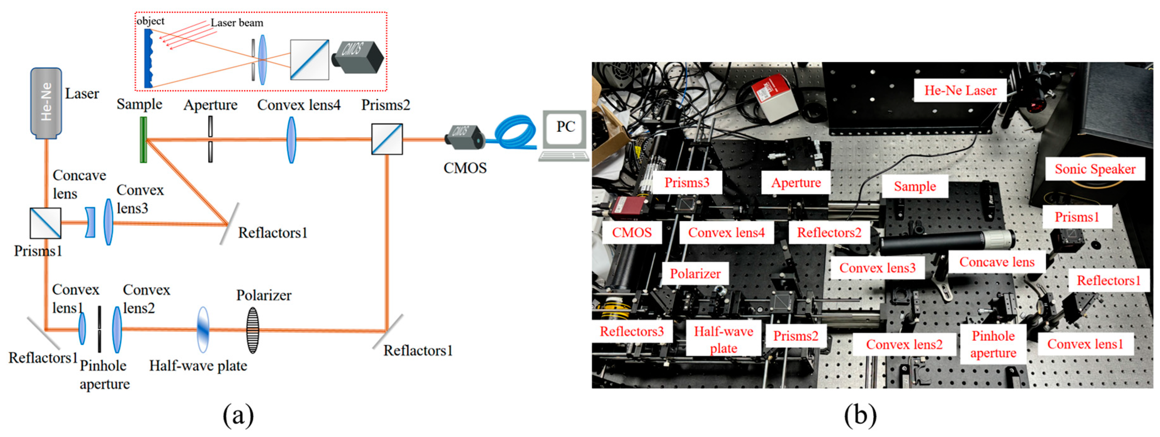
4.1. Optimized System Design

The optical setup of the digital holographic system is composed of a digital holographic interference system and a vibration excitation source, as shown in Figure 6. The light source is a helium–neon laser of 632.8 nm wavelength; the CMOS camera model used is Manta G-419B of 2048 × 2048 pixels from Allied Vision in Stadtroda, Germany. The camera’s supporting image acquisition software is Vimba Viewer, which collects holograms by adjusting the exposure time. The vibration excitation source is an audio signal generator and a supporting speaker from NTI. The frequency range of the audio signal generator is 10 Hz–20 kHz, and the sine wave signal and sweep mode can be adjusted. When the object is irradiated with coherent light, speckle patterns are obtained on the image plane. A 30 mm plano-convex lens, a 5 µm pinhole aperture, and a 200 mm cemented achromatic lens from lbtek (Changsha, China) are adopted to form a Kepler beam expander to filter stray light.

The optical system is optimized. First, a plano-convex lens with a focal length of 100 mm is placed between the camera and the object under test. By adjusting the positions of the three, the pure object light spectrum appears as a bright circular spot as shown in Figure 7a. The reference light spectrum is obtained as shown in Figure 7b. A polarizer and a half-wave plate are used to attenuate the light intensity and adjust the light intensity ratio, so that contrast of the interferograms can be guaranteed.

The off-axis angle is adjusted so that the object wave and reference wave can be separated in the spectrum domain, as shown in Figure 7c. Based on the double exposure method, two interference images before and after vibration deformation are recorded, and the deformation of the vibrating object is obtained by calculating the phase difference between the two interference images. After acoustic wave excitation, the surface of the object will produce deformation displacement, and the amplitude of the defect will be significantly different from the surrounding area. Therefore, defect identification can be achieved based on the abnormal areas of the phase differences.

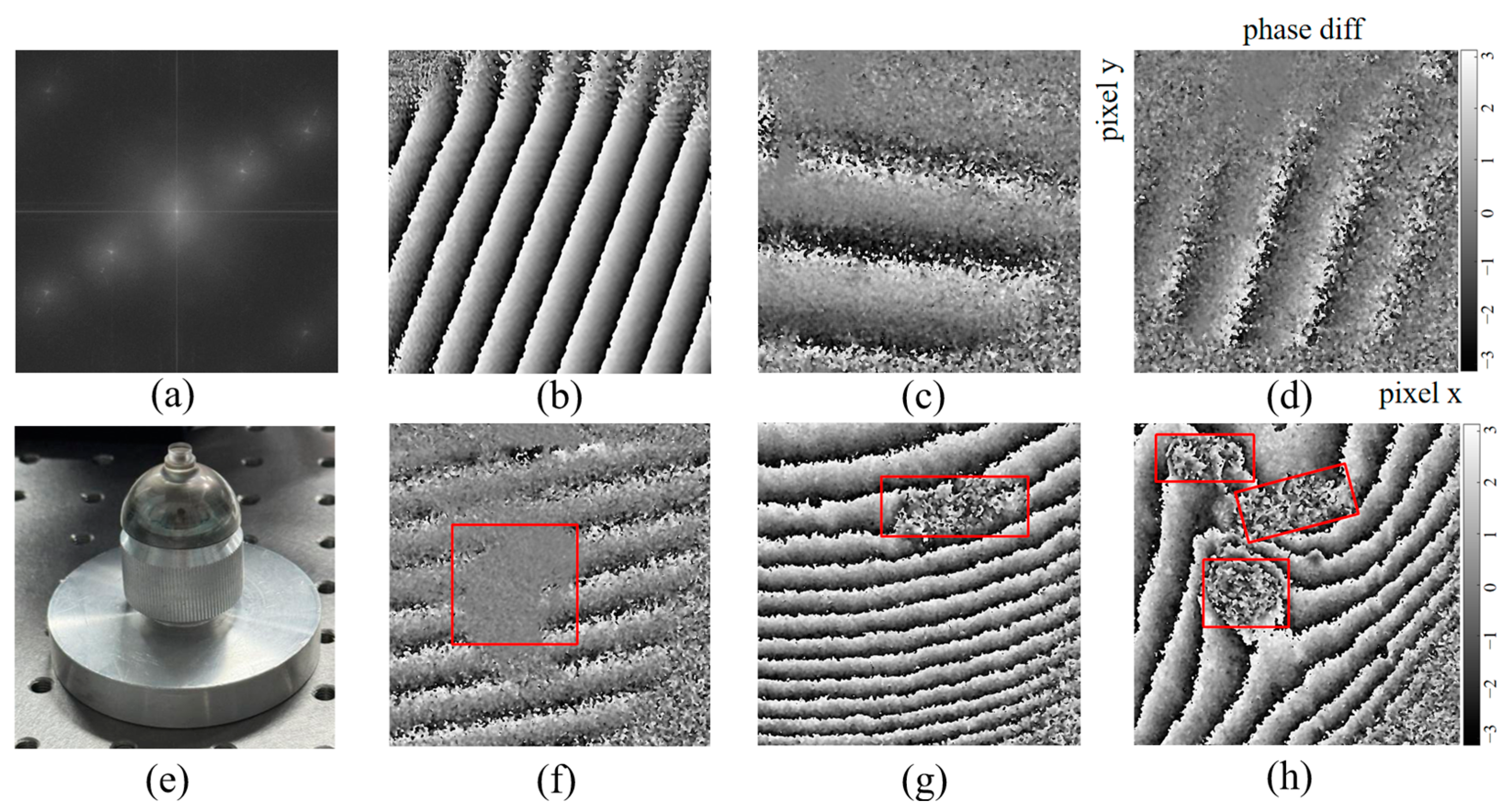
4.2. Defect Recognition

The actual phase difference before and after the vibration can be expressed as follows [29]:

$$\begin{array}{ll}\Delta \varphi (x,y)& ={\varphi }_{vib}(x,y)-{\varphi }_{ref}(x,y)\\ & =\arctan {\displaystyle \frac{\mathrm{Im}\left[U_{ref}^{*}(x,y)\cdot U_{vib}(x,y)\right]}{\mathrm{Re}\left[U_{ref}^{*}(x,y)\cdot U_{vib}(x,y)\right]}}\end{array}$$

(9)

where $U_{ref}(x,y)$ and $U_{vib}(x,y)$ are the complex amplitudes reconstructed from the holograms before and after vibration, respectively.

The sine-cosine transform method is applied to denoise the phase difference before and after vibration, and some of the results are shown in Figure 8. At the same time, some profiles are plotted to intuitively reveal the filtering effect. Among them, the green line is the manual drawing line, and Figure 8(c1,c2,d1,d2) illustrates the distribution of phase values along this line before and after filtering.

To evaluate the sensitivity in identifying vibration deformation, preliminary verification experiments were conducted. First, the positive and negative first-order spectra are completely separated from the zero-order spectrum by adjusting the off-axis angle. In the completely separated state, the spectrum diagram obtained by Fourier transform is shown in Figure 9a. It can be seen that there is basically no aliasing between the items. The resulting phase difference is shown in Figure 9b, where the clear fringe pattern confirms that the setup can accurately detect small deformations.

The hemispherical resonator gyro, a key component in inertial navigation systems, is typically made of quartz with a metal coating, as shown in Figure 9e. Since the resonator has a fixed vibrating frequency, the amplitude distribution of the resonator is measured, thereby further proving the measurement capability. First, the resonator is fixed so that the illumination beam is aligned with the center and a static state hologram is collected. The vibration state hologram is collected after the resonator is vibrated. The amplitude distribution is calculated by the phase difference before and after the vibration, as shown in Figure 9c,d. The gradual increase in amplitude across the resonator surface, with well-defined interference fringes, demonstrates the high sensitivity of the proposed method.

Since micro-defects may appear in optical materials over time, their influence on vibration behavior is also investigated. A 100 µm aperture was tested, and the phase difference before and after vibration is presented in Figure 9f, showing a distinct amplitude variation at the defect position marked by the red square frame. Further tests are conducted on polymer plates with one and three artificial through-holes, with results shown in Figure 9g,h. The method demonstrates a high sensitivity in detecting through-hole defects, confirming its effectiveness in identifying local anomalies in optical materials.

To verify the effectiveness of the proposed method in detecting defects in optical materials, a polymer plate sample with subsurface defects was fabricated. A confocal microscope Olympus LEXT 4200 was used to measure the sample as well, as shown in Figure 10a. The obtained surface morphology distribution is shown in Figure 10b, where there is no obvious abnormity, revealing that confocal microscopy fails to detect subsurface defects. In contrast, the results of the proposed method are illustrated in Figure 10(c1,c2,d1,d2). The results show that neither the hologram nor the complex amplitude distribution directly reveal the defect, indicating that conventional holographic interferometry alone is insufficient for defect detection. However, the phase difference map between pre- and post-vibration states in Figure 10e clearly highlights the defects while marked by the red square frame. This demonstrates that identifying defect regions through phase difference analysis is both necessary and effective.

Furthermore, infrared thermography [33] and laser ultrasonics [34] are two commonly used methods for defect detection, but they suffer from shortcomings. Infrared thermography requires laser excitation or heating to analyze the impact of defects. However, when detecting some materials like 3D printed glass, its long absorption wavelength makes it difficult to find a suitable laser source with the required power and wavelength. On the contrary, laser ultrasonics relies on pulsed laser excitation to generate ultrasonic waves, and defects are detected by analyzing their effect on wave propagation. However, due to the low absorption and conversion efficiency of 3D printed glass to common laser energy, the detecting sensitivity is limited. Therefore, these two methods cannot be widely adopted for testing optical materials.

The structural integrity of optical sandwich composite materials depends on the close bonding between the layers of materials. Surface defects, internal debonding, and subsurface defects will affect their optical properties. The experimental setup was used to analyze simplified double-layer bonded polymer plates, as shown in Figure 11a. The sample to be tested is placed at a position of clear imaging. First, the interference pattern of the sample in a static state is captured. Then, the frequency of the sine wave is changed by the acoustic wave excitation device. The phase difference before and after vibration is obtained by the double exposure method. The phase difference associated with different positions is shown in Figure 11b,c. It can be seen that there is an obvious amplitude abnormity at the position of the surface depression which is marked by the red square frame.

The internal debonding defects of optical adhesive materials will affect the scattering and light transmission properties of light, and will also affect the overall mechanical strength. Internal debonding is artificially created in the adhesive layer of the double-layer adhesive polymer plate, while ensuring that these defects are invisible from the surface. The frequency band when the vibration amplitude is large is determined by frequency sweeping. In this frequency band, samples with internal debonding at different locations are acoustically excited, and the phase difference diagrams before and after vibration are measured, as shown in Figure 11d,e. It can be seen that as the internal debonding location changes, the deformation abnormity also changes, and this method can be used to identify the internal debonding location.

In this study, a honeycomb sandwich-bonded polymer plate with artificially introduced subsurface hole defects at different positions on the back side is investigated. Holograms of the defective sample before and after vibration are collected at different acoustic excitation frequencies (200, 225, 250, and 275 Hz). As shown in Figure 12(a1,b1,c1,d1), the phase difference fringe density initially increases with the excitation frequency, reaches a maximum value at resonance, and then decreases. This is because the resonant frequency of the area around the defect of the sample falls within the excitation range, resulting in a significant increase in the vibration amplitude. Figure 12(a2,b2,c2,d2) shows that the highest fringe density on both sides of the defect occurs at 250 Hz, while Figure 12(a3,b3,c3,d3) shows that the fringe density around the defect gradually increases with frequency. Regardless of the change in fringe density, the fringe anomality corresponding to the subsurface hole remains unchanged, indicating that the defect area which marked by the red square frame has obvious amplitude and resonant frequency characteristics. These findings confirm that the subsurface defect can be identified correctly based on the amplitude anomality.

Laser powder bed fusion (LPBF) technology is widely used in metal manufacturing. In recent years, it has been extended to glass processing due to the demand for personalization and complex structures. However, the special physical and chemical properties of quartz glass pose challenges to the LPBF process. Reducing the strip width can optimize the molding quality, but is prone to processing marks at the beginning of the scan because of the uneven heat distribution due to the difference in thermal conductivity between the formed glass and the unmelted powder. In this study, acoustic waves are used to excite the vibration of the glass surface, and the phase difference before and after the vibration is calculated. It is found that the amplitude of the stress concentration area which marked by the red square frame is abnormal, corresponding to the microstructure, as illustrated in Figure 13a. Phase difference fringes can reveal the processing marks of 3D printed glass and provide a reference for optimizing laser processing parameters.

5. Conclusions

In this paper, a time-averaged digital holographic measurement system was designed and optimized for defect identification in optical materials. Finite element simulations proved that the resonance frequency of the defect region differs from that of the surrounding material, resulting in local amplitude abnormities. The experimental setup ensured effective recording by extending the camera exposure time. By combining double exposure holography with phase extraction technology, the phase difference distribution can be obtained, so that defects can be precisely identified by phase difference image anomality. This study provides a non-destructive and highly sensitive method for assessing the fabricating quality of key functional optical components.

References

1. Kumar, M.; Pensia, L.; Kumar, R. Highly stable vibration measurements by common-path off-axis digital holography. Opt. Lasers Eng. 2023, 163, 107452. [Google Scholar] [CrossRef]
2. Kumar, M.; Matoba, O. 2D full-field displacement and vibration measurements of specularly reflecting surfaces by two-beam common-path digital holography. Opt. Lett. 2021, 46, 5966–5969. [Google Scholar] [CrossRef] [PubMed]
3. De Greef, D.; Soons, J.; Dirckx, J.J.J. Digital stroboscopic holography setup for deformation measurement at both quasi-static and acoustic frequencies. Int. J. Optomechatronics 2014, 8, 275–291. [Google Scholar] [CrossRef]
4. Kakue, T.; Endo, Y.; Nishitsuji, T.; Shimobaba, T.; Masuda, N.; Ito, T. Digital holographic high-speed 3D imaging for the vibrometry of fast-occurring phenomena. Sci. Rep. 2017, 7, 10413. [Google Scholar] [CrossRef]
5. Khaleghi, M.; Guignard, J.; Furlong, C.; Rosowski, J.J. Simultaneous full-field 3-D vibrometry of the human eardrum using spatial-bandwidth multiplexed holography. J. Biomed. Opt. 2015, 20, 111202. [Google Scholar] [CrossRef]
6. Rajput, S.K.; Matoba, O.; Kumar, M.; Quan, X.; Awatsuji, Y. Sound wave detection by common-path digital holography. Opt. Lasers Eng. 2021, 137, 106331. [Google Scholar] [CrossRef]
7. Powell, R.L.; Stetson, K.A. Interferometric vibration analysis by wavefront reconstruction. J. Opt. Soc. Am. 1965, 55, 1593–1598. [Google Scholar] [CrossRef]
8. Picart, P.; Leval, J.; Mounier, D.; Gougeon, S. Time-averaged digital holography. Opt. Lett. 2003, 28, 1900–1902. [Google Scholar] [CrossRef]
9. Singh, V.R.; Miao, J.; Wang, Z.; Hegde, G.; Asundi, A. Dynamic characterization of MEMS diaphragm using time averaged in-line digital holography. Opt. Commun. 2007, 280, 285–290. [Google Scholar] [CrossRef]
10. Bruno, F.; Laurent, J.; Prada, C.; Lamboul, B.; Passilly, B.; Atlan, M. Non-destructive testing of composite plates by holographic vibrometry. J. Appl. Phys. 2014, 115, 154503. [Google Scholar] [CrossRef]
11. Psota, P.; Ledl, V.; Dolecek, R.; Erhart, J.; Kopecky, V. Measurement of piezoelectric transformer vibrations by digital holography. IEEE Trans. Ultrason. Ferroelectr. Freq. Control 2012, 59, 1962–1968. [Google Scholar] [CrossRef] [PubMed]
12. Psota, P.; Lédl, V.; Matoušek, O.; Doleček, R.; Kredba, J. Pixel-wise Amplitude Distribution Evaluation in Time Average Digital Holography. J. Phys. Conf. Ser. 2018, 1149, 012033. [Google Scholar] [CrossRef]
13. Psota, P.; Mokrý, P.; Lédl, V.; Stašík, M.; Matoušek, O.; Kredba, J. Absolute and pixel-wise measurements of vibration amplitudes using time-averaged digital holography. Opt. Lasers Eng. 2019, 121, 236–245. [Google Scholar] [CrossRef]
14. Fu, M.; Dornseiff, J.; Barth, V.; Scheer, E. Time-averaged interference fringe analysis: A quantitative study of nanomembrane vibration dynamics. Sens. Actuators A Phys. 2025, 383, 116172. [Google Scholar] [CrossRef]
15. Pavillon, N.; Arfire, C.; Bergoënd, I.; Depeursinge, C. Iterative method for zero-order suppression in off-axis digital holography. Opt. Express 2010, 18, 15318–15331. [Google Scholar] [CrossRef]
16. Colomb, T.; Kühn, J.; Charrière, F.; Depeursinge, C.; Marquet, P.; Aspert, N. Total aberrations compensation in digital holographic microscopy with a reference conjugated hologram. Opt. Express 2006, 14, 4300–4306. [Google Scholar] [CrossRef]
17. Weng, J.; Li, H.; Zhang, Z.; Zhong, J. Design of adaptive spatial filter at uniform standard for automatic analysis of digital holographic microscopy. Optik 2014, 125, 2633–2637. [Google Scholar] [CrossRef]
18. He, X.; Nguyen, C.V.; Pratap, M.; Zheng, Y.; Wang, Y.; Nisbet, D.R.; Williams, R.J.; Rug, M.; Maier, A.G.; Lee, W.M. Automated Fourier space region-recognition filtering for off-axis digital holographic microscopy. Biomed. Opt. Express 2016, 7, 3111–3123. [Google Scholar] [CrossRef]
19. Li, J.; Wang, Z.; Gao, J.; Liu, Y.; Huang, J. Adaptive spatial filtering based on region growing for automatic analysis in digital holographic microscopy. Opt. Eng. 2015, 54, 031103. [Google Scholar] [CrossRef]
20. Dang, C.; Li, J.; Zhao, P.; Xu, T. Adaptivly locating holographic positive first-order spectrum using maximum value of spectral phase. Opt. Precis. Eng. 2022, 30, 1272–1281. [Google Scholar] [CrossRef]
21. Yan, K.; Yu, Y.; Sun, T.; Asundi, A.; Kemao, Q. Wrapped phase denoising using convolutional neural networks. Opt. Lasers Eng. 2020, 128, 105999. [Google Scholar] [CrossRef]
22. Wang, Z.; Hu, S.; Xia, Z.; Sun, Z.; Yang, L. DSPI image denoising method based on sine-cosine decomposition and BM3D filtering. Autom. Instrum. 2021, 6, 1–6. [Google Scholar]
23. Xiao, Q.; Fan, M.; Zuo, X. Speckle phase map denoising based on empirical wavelet transform and cross correlation. Opt. Eng. 2021, 60, 064102. [Google Scholar] [CrossRef]
24. Niu, R.; Tian, A.L.; Wang, D.S.; Liu, B.C.; Wang, H.J.; Qian, X.T.; Liu, W.G. Speckle Noise Suppression of Digital Holography Measuring System. Laser Optoelectron. Prog. 2022, 59, 1609002. [Google Scholar]
25. Chen, J.; Liao, H.; Kong, Y.; Zhang, D.; Zhuang, S. Speckle denoising based on Swin-UNet in digital holographic interferometry. Opt. Express 2024, 32, 33465–33482. [Google Scholar] [CrossRef]
26. Thomas, B.P.; Annamala Pillai, S.; Narayanamurthy, C.S. Investigation on vibration excitation of debonded sandwich structures using time-average digital holography. Appl. Opt. 2017, 56, F7–F13. [Google Scholar] [CrossRef]
27. Mancio, L.; Olivares-Perez, A. Complete description of effects on reconstruction of dynamic objects from time-averaged digital holography to high-speed digital holography. Opt. Contin. 2024, 3, 893–901. [Google Scholar] [CrossRef]
28. Asundi, A.; Singh, V.R. Time-averaged in-line digital holographic interferometry for vibration analysis. Appl. Opt. 2006, 45, 2391–2395. [Google Scholar] [CrossRef]
29. Liu, Y.; Jiang, Z.; Wang, Y.; Sun, Q.; Chen, H. Single-frame reconstruction for improvement of off-axis digital holographic imaging based on image interpolation. Opt. Lett. 2020, 45, 6623–6626. [Google Scholar] [CrossRef]
30. Ning, X.; Li, W.; Wu, S.; Dong, M.; Zhu, L. Fast phase denoising using stationary wavelet transform in speckle pattern interferometry. Meas. Sci. Technol. 2019, 31, 025205. [Google Scholar] [CrossRef]
31. Xiao, Q.; Li, J.; Zeng, Z. A denoising scheme for DSPI phase based on improved variational mode decomposition. Mech. Syst. Signal Process. 2018, 110, 28–41. [Google Scholar] [CrossRef]
32. Ding, J.; Zhou, W.; Yu, Y.J. Vibration Modes Study of Defective Eardrum Realized Using Digital Holographic Endoscopy. Chin. J. Lasers 2023, 50, 1507204. [Google Scholar]
33. Mevissen, F.; Meo, M. Ultrasonically stimulated thermography for crack detection of turbine blades. Infrared Phys. Technol. 2022, 122, 104061. [Google Scholar] [CrossRef]
34. Yu, J.; Zhang, D.; Li, H.; Song, C.; Zhou, X.; Shen, S.; Zhang, G.; Yang, Y.; Wang, H. Detection of Internal Holes in Additive Manufactured Ti-6Al-4V Part Using Laser Ultrasonic Testing. Appl. Sci. 2020, 10, 365. [Google Scholar] [CrossRef]
Figure 1. Schematic diagram of spectrum filtering; (a) spectral distribution; (b) spectrum extraction; (c) eliminate the carrier.
Photonics 12 00373 g001
Figure 2. Analysis of the influence of circular hole defects and subsurface defects on the vibrating amplitude: (a1) measurement points around the circular hole defect; (a2) subsurface defects; (b1,c) difference of vibration displacements; (b2) vibration displacement changes with and without subsurface defects.
Photonics 12 00373 g002
Figure 3. Effects of circular hole defects of different depths and crack defects of different lengths on the vibration displacements: (a1) circular hole defects of different depths; (b1) vibration displacements associated with different hole depths; (a2) crack defects of different lengths; (b2) vibration displacements associated with different crack lengths.
Photonics 12 00373 g003
Figure 4. Relationship between amplitude envelope and exposure time. (a) Short exposure time; (b) long exposure time.
Photonics 12 00373 g004
Figure 5. Comparison of holographic fringes at different exposure times. (a) 0.08 T, (b) 0.12 T, (c) 0.25 T, (d) 0.50 T, (e) 0.67 T, (f) T, (g) 2 T, (h) 3 T, and (i) 4 T.
Photonics 12 00373 g005
Figure 6. Setup of reflective digital holographic system: (a) optical diagram; (b) actual setup.
Photonics 12 00373 g006
Figure 7. Spectrum diagram of the holograms: (a) object light spectrum; (b) reference light spectrum; (c) spectrum separation by adjusting the off-axis angle.
Photonics 12 00373 g007
Figure 8. Sincosine transform combined with BM3D noise reduction effect diagram; (a1,a2) noise phase difference diagram; (b1,b2) phase difference diagram after noise reduction; (c1d2) phase distribution profiles before and after noise reduction.
Photonics 12 00373 g008
Figure 9. Detecting sensitivity verification: (a) spectrum separation diagram of the reflector; (b) phase difference before and after tilt; (c,d) amplitude distribution of resonator; (e) actual image of the resonator; (f) phase difference before and after vibration; (g,h) phase difference of polymer plastic plate.
Photonics 12 00373 g009
Figure 10. Comparison of different defect detecting methods: (a) confocal microscope; (b) confocal microscope result; (c1,c2) interference hologram before and after vibration; (d1,d2) reconstructed complex amplitude before and after vibration; (e) phase difference diagram before and after vibration after filtering.
Photonics 12 00373 g010
Figure 11. Defect identification of optical sandwich composite materials: (a) defects in sandwich adhesive materials, (b,c) phase difference diagrams of samples with surface depression defects before and after vibration; (df) phase difference diagrams of samples with debonding defects on the left, middle, and right sides, respectively.
Photonics 12 00373 g011
Figure 12. Subsurface defect identification at different locations of polymer plastic plates. (a1a3) Phase difference diagrams before and after vibration at an acoustic excitation frequency of 200 Hz; (b1b3) 225 Hz; (c1c3) 250 Hz; (d1d3) 275 Hz.
Photonics 12 00373 g012
Figure 13. 3D printed glass processing trace identification diagram: (a) 3D printed glass microstructure; (b) processing trace identification.
Photonics 12 00373 g013
Disclaimer/Publisher’s Note: The statements, opinions and data contained in all publications are solely those of the individual author(s) and contributor(s) and not of MDPI and/or the editor(s). MDPI and/or the editor(s) disclaim responsibility for any injury to people or property resulting from any ideas, methods, instructions or products referred to in the content.