Study on the Wavelength-Dependent Temporal Waveform Characteristics of a High-Pressure CO₂ Master Oscillator Power Amplifier System

Abstract

This study systematically investigates the temporal characteristics of a high-pressure CO₂ master oscillator power amplifier (MOPA) system under tunable spectral lines. Based on a continuously tunable CO₂ oscillator–amplifier system, we experimentally measured the variation in the laser pulse width before and after amplification at different spectral lines, with the oscillator and amplifier operating at pressures of 7 atm and 3 atm, respectively. The results indicate that, for most spectral lines, the laser pulse width remained nearly unchanged after amplification. However, at certain spectral lines, a distinct phenomenon was observed: pulse broadening for strong lines and pulse narrowing for weak lines. To explain this phenomenon, theoretical calculations were conducted based on a high-pressure CO₂ six-temperature model, and the experimental results were analyzed from the perspective of small-signal gain dynamics. This study reveals that variations in the laser pulse width primarily originated from differences in the gain build-up time across different spectral lines, which in turn influenced the amplification of both the pulse pedestal and the main pulse. For strong spectral lines, the amplifier gain built up rapidly, leading to more uniform amplification of the entire laser pulse and resulting in pulse broadening. Conversely, for weak spectral lines, the amplifier gain built up more slowly, with amplification primarily concentrated in the main pulse, causing a reduction in the pulse width. This finding has significant implications for optimizing narrow-pulse CO₂ lasers and provides crucial insights into the temporal characteristics of applications, such as laser isotope separation and extreme ultraviolet (EUV) light source generation.

1. Introduction

CO₂ pulse lasers, with their exceptional peak power and pulse energy, are widely used in fields such as isotope separation [1,2] and extreme ultraviolet (EUV) light sources [3,4]. In these applications, the laser pulse width and peak power are key parameters for evaluating performance. In molecular laser isotope separation (MLIS) technology, CO₂ lasers precisely control the isotope separation process by manipulating the formation and desorption of adsorbate clusters between molecules and the carrier gas. This method is commonly referred to as the “molecular method” [5]. Research by Ryan Snyder and others has shown that the laser pulse width directly influences the energy flow parameters, particularly in enhancing the effective utilization of photon numbers and meeting the peak power threshold required for Raman scattering [6]. Studies have demonstrated that for a tail-free 80 ns pulse, the pulse energy needs to reach nearly 400 mJ to meet the minimum threshold for uranium MLIS. In the EUV light source field, CO₂ pulse lasers with a wavelength of 10.6 µm are focused onto a tin (Sn) target to generate highly ionized plasma, which then emits EUV light at a wavelength of 13.5 nm [7]. The conversion efficiency and output power of EUV light sources are affected by multiple physical processes, with the CO₂ laser pulse width and its temporal waveform playing a crucial role. According to research by Alexander and others [8], the pulse width and temporal waveform of CO₂ lasers directly influence the surface morphology of the target, thereby affecting EUV light source conversion efficiency and output power.

However, traditional TEA CO₂ lasers often suffer from discharge and relaxation effects, leading to significant tailing. To overcome this, master oscillator power amplifier (MOPA) systems are employed, which enable high peak power and tail-free pulses [9].

CO₂ MOPA systems have gained significant attention. For instance, in 1999, S.Y. Tochitsky and colleagues reported a terawatt-level CO₂ laser capable of generating ultra-short pulses [10]. This system was capable of generating ultra-short pulses with a pulse width of 160 ps and a peak power of 1.1 TW. In 2010, the Neptune Laboratory further studied the effect of collision broadening under high-pressure conditions on output pulse modulation distributions [11]. In 2020, M.N. Polyanskiy and others reported a picosecond terawatt-level long-wave infrared (LWIR) laser system at Brookhaven National Laboratory’s accelerator facility in the United States [12]. This system uses a two-stage amplification design, effectively reducing the seed laser’s linewidth to approximately 100 nm, which in turn reduces the modulation distribution of the gain spectrum at the target center wavelength of 9.3 μm, significantly suppressing the pulse train output in the oscillation–amplification system.

Recent studies have investigated the gain characteristics of CO₂ amplifiers and their effects on laser temporal waveforms. Feldman et al. (1975) established a theoretical model for short-pulse amplification [13], while Zhang et al. (2021) numerically simulated population inversion dynamics in a 4 kW axial-flow amplifier, revealing the evolution of pulse waveforms from a gain perspective [14]. Notably, their work did not address the spectral line-dependent variations in temporal waveforms or the effects of gain saturation. Ye et al. (2023) further explored pressure-dependent gain spectra but focused less on the temporal characteristics of the pulses [15]. Despite these efforts, two critical gaps remain: (1) a systematic analysis of temporal waveform evolution across different spectral lines, and (2) a quantitative evaluation of the impact of gain saturation on amplified pulses.

To bridge these gaps, this paper, based on a continuously tunable high-pressure CO₂ oscillator–amplifier system, measures the laser pulse width at different wavelengths before and after amplification to investigate how the amplification process affects the temporal waveform. Additionally, using the high-pressure CO₂ six-temperature model, the small-signal gain of the CO₂ laser at different spectral lines was calculated to theoretically analyze the variation in pulse width for the strong line (e.g., 10P(20)) and weak line (e.g., 10P(10)) after amplification. Furthermore, based on the characteristics of gain saturation, the changes in time-domain waveforms at different spectral lines are discussed in stages. By addressing these gaps, we hope to contribute valuable insights into the optimization of CO₂ laser systems for both scientific research and practical applications.

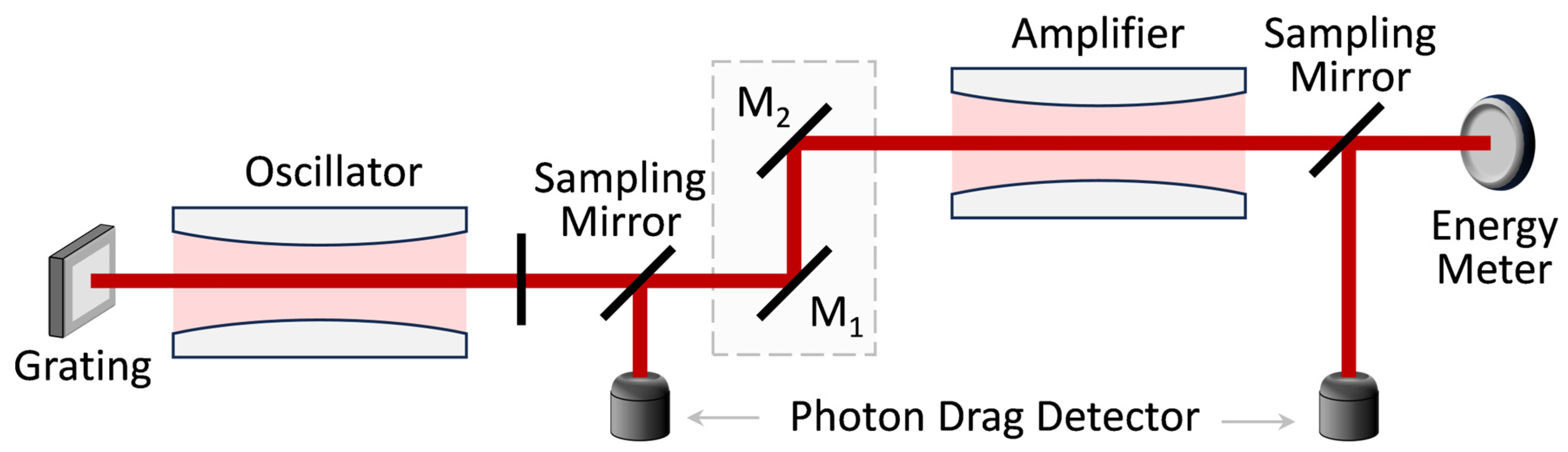
2. Experimental Setup

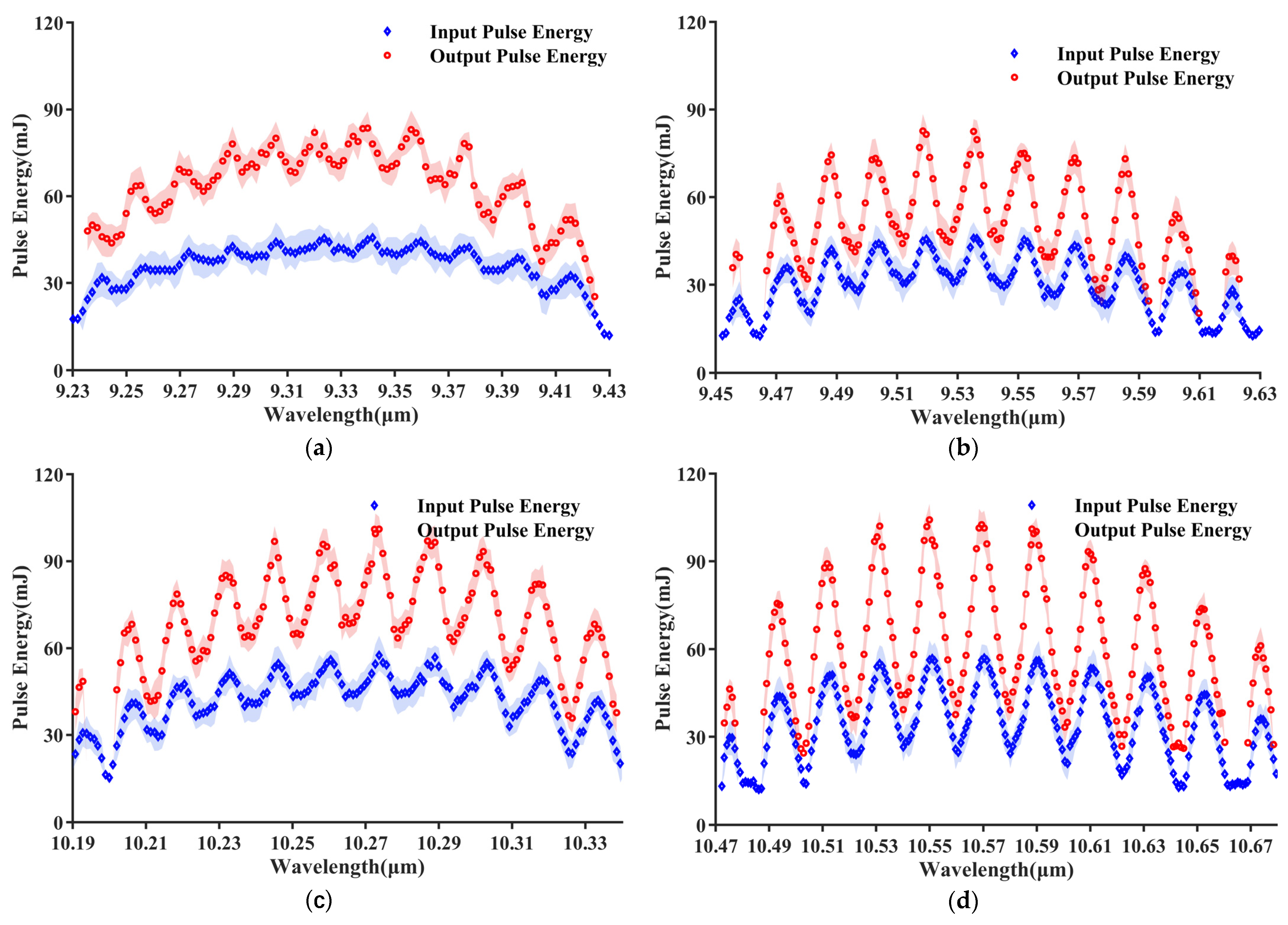
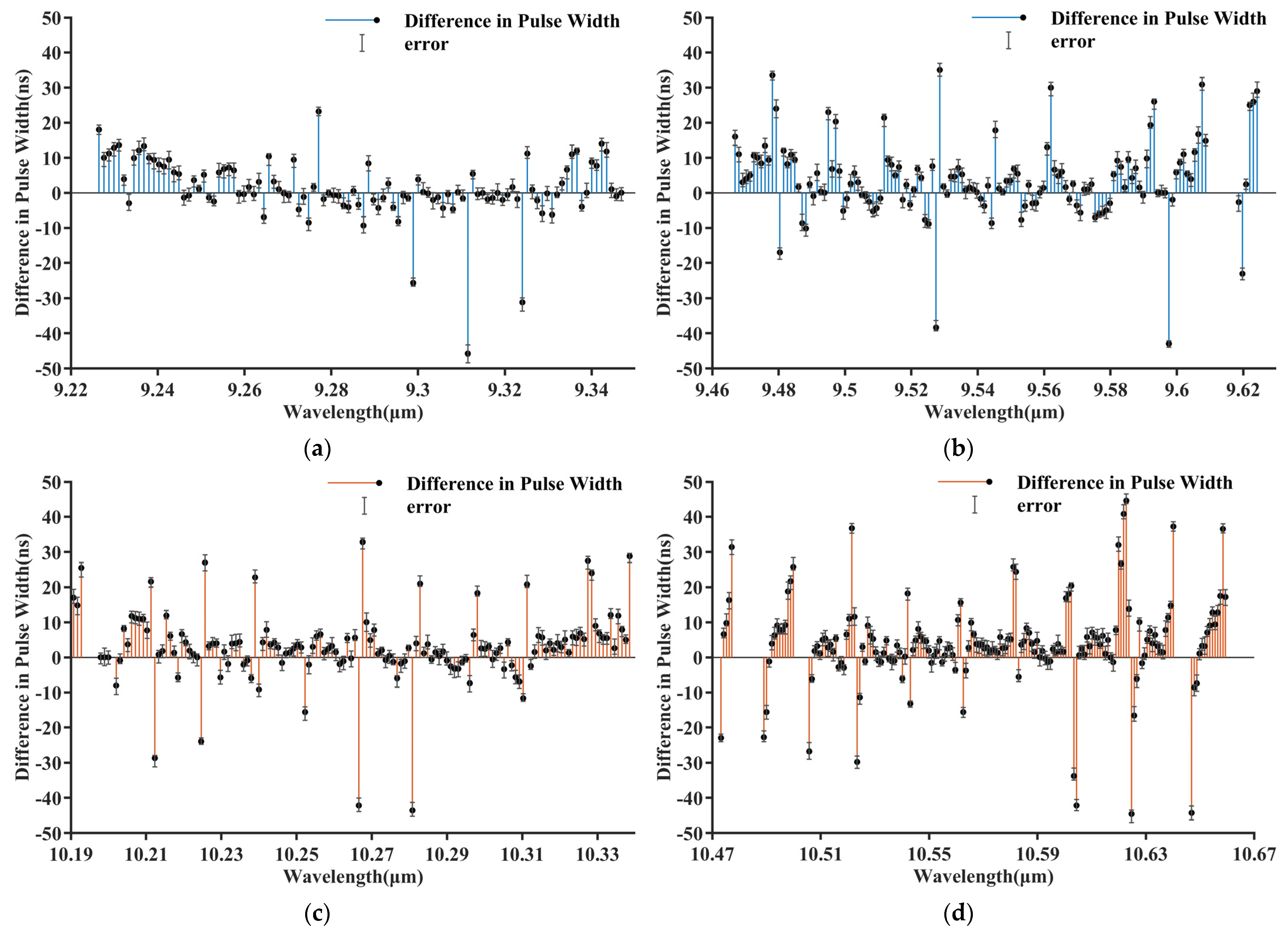
The experimental system consisted of three main components: a discharge control unit, two laser cavities, and measurement equipment. A schematic diagram of the setup is shown in Figure 1. The controller regulated the operating voltage applied to the energy storage capacitor while simultaneously providing two trigger signals. These pulse signals activated the thyristor, closing the circuit and discharging the stored energy from the capacitor into the laser cavity, thereby generating laser output. The operating voltage was adjustable from 0 kV to 70 kV, with the energy storage capacitor having a capacitance of 4.7 nF, allowing for a maximum injected energy of 11.52 J.

Both the laser oscillator and amplifier employed cylindrical steel cavities. Thickened zinc selenide (ZnSe) Brewster windows were used at each end for sealing and as input and output windows for linearly polarized laser beams. The Brewster windows were arranged symmetrically to counteract optical axis deviations caused by refractive index effects when passing through a single window.

The laser oscillator utilized a plano-concave resonator design with a cavity length of 0.8 m. It consisted of a ZnSe output coupler (reflectivity R = 80%) and a diffraction grating operating at the Littrow angle, with a grating constant of 1/150 mm. The gain regions of the laser oscillator and amplifier were 7 mm × 7 mm × 380 mm and 20 mm × 20 mm × 600 mm, respectively. The laser power was amplified using a traveling-wave amplification scheme, where the angles of two mirrors (M1 and M2) were adjusted to ensure that the laser beam from the oscillator entered the amplifier cavity at normal incidence.

ZnSe sampling mirrors were placed at both the oscillator and amplifier output positions to measure the laser energy and pulse width before and after amplification. In the experiment, a Hamamatsu B749 photon-drag detector (Hamamatsu Photonics K.K., Hamamatsu City, Japan) and a Tektronix DPO4104B digital phosphor oscilloscope (Tektronix, Inc., Beaverton, OR, USA) were used to record the pulse waveforms. The pulse energy was measured using a Coherent J100MB energy probe (Coherent, Inc., Santa Clara, CA, USA) and a Coherent EPM2000 power meter (Coherent, Inc., Santa Clara, CA, USA).

3. Results

To investigate the amplification effect of a high-pressure CO₂ amplifier on laser pulses at different wavelengths and to analyze the temporal distribution characteristics of laser pulses before and after amplification, we conducted experimental measurements of the pulse energy and pulse width.

In the experiment, a controller synchronously output two TTL signals to trigger both the laser oscillator and the amplifier. Upon triggering, the oscillator underwent free oscillation to generate the seed laser, which was spectrally selected by a diffraction grating before output. The laser pulse was then directed into the amplifier cavity at normal incidence, with its angle adjusted by two mirrors (M1 and M2). A preset delay between the trigger signals ensured that the amplifier was activated after the seed laser had been generated, thereby providing gain for traveling-wave amplification of the seed pulse. The laser energy and pulse width before and after amplification were sampled and measured using two beam splitters, enabling the quantification of temporal variations in laser pulses across different spectral lines.

The experimental conditions were as follows: The high-pressure CO₂ laser operated at a voltage of 50 kV with a working pressure of 7 atm, using a gas mixture composition of CO₂:N₂:He = 2:1:16. The high-pressure CO₂ amplifier operated at a voltage of 60 kV with a working pressure of 3 atm, with a gas mixture composition of CO₂:N₂:He = 1:1:16.

To achieve a sufficient gain length, the electrode spacing in the amplifier was increased to 20 mm, compared to 7 mm in the oscillator. Given this adjustment, to ensure adequate excitation efficiency and maintain an appropriate E/N ratio (the ratio of electric field strength E to the CO₂ particle number density N), the proportion of CO₂ molecules in the amplifier gas mixture was correspondingly reduced. As a result, the gas compositions of the amplifier and the laser oscillator differed.

The experimental results are presented in Figure 2 and Figure 3.

Figure 2 illustrates the variation in laser output energy as a function of the grating-tuned wavelength. Due to the limitations of the energy meter’s measurement range, experimental data in the low-energy region are somewhat incomplete. The results reveal that the laser output energy exhibited distinct periodic oscillations, with particularly pronounced fluctuations in specific wavelength regions.

In the “strong-line” region of the CO₂ laser spectrum, the output energy increases significantly, displaying clear peak characteristics. Simultaneously, within this wavelength range, the energy amplification factor of the amplifier for the seed laser is relatively high, indicating that the amplifier provided enhanced gain to the seed laser in this region. In contrast, in the “weak-line” region, the laser output energy decreases markedly, forming troughs, and the corresponding energy amplification factor of the amplifier is notably lower. This suggests that the amplifier’s gain effect on the seed laser was relatively weaker in this spectral range. Through calculations, the maximum single-pass energy amplification factor across the entire tuning bandwidth was found to be 2.16, with the corresponding maximum amplifier gain being 1.28% cm⁻¹.

Figure 3 illustrates the variation in laser pulse width as a function of the grating-tuned wavelength. Overall, the pulse width remains relatively stable across most of the spectral bandwidth, with consistent temporal characteristics. However, significant fluctuations in the pulse width are observed at certain spectral lines.

In the “weak-line” regions at the edges of each spectral band, the pulse width narrows significantly after amplification. For example, in the 9R band, narrowing occurs in the 9.224–9.234 μm and 9.336–9.346 μm regions; in the 9P band, in the 9.466–9.478 μm range; and in the 10R band, from 10.180 μm to 10.214 μm. Additionally, similar narrowing phenomena are observed in the 10P band, particularly in the 10.472–10.504 μm and 10.646–10.678 μm ranges.

Conversely, in the “strong-line” regions at the centers of each band, the pulse width broadens after amplification. For instance, in the center of the 10P band, pulse width broadening is observed in the 10.506–10.512 μm, 10.524–10.532 μm, 10.542–10.550 μm, 10.562–10.578 μm, 10.584–10.590 μm, and 10.606–10.614 μm ranges.

To more clearly demonstrate the changes in the pulse width before and after amplification at different wavelengths, the actual measured pulse width data for wavelengths with significant variations are presented in

Table 1. Measured pulse widths before and after amplification at wavelengths with significant changes.

Spectral Band (μm)	Before Amplification (ns)	After Amplification (ns)
9.277	64.8	88
9.299	93.5	67.8
9.311	121.8	76
9.324	118.4	87.2
9.478	115.5	149
9.527	124.6	86.2
9.528	93	128
9.597	174	131
9.607	114	144.9
10.212	157.7	129
10.226	105	132.4
10.266	115	72.8
10.268	70.2	103
10.281	141	97.4
10.522	84	120.7
10.524	131	101.2
10.602	147	93.2
10.603	151	88.8
10.621	97	137.8
10.622	125	169.6
10.625	160	115.4

. This table lists the specific experimental measurements.

4. Analysis and Discussion

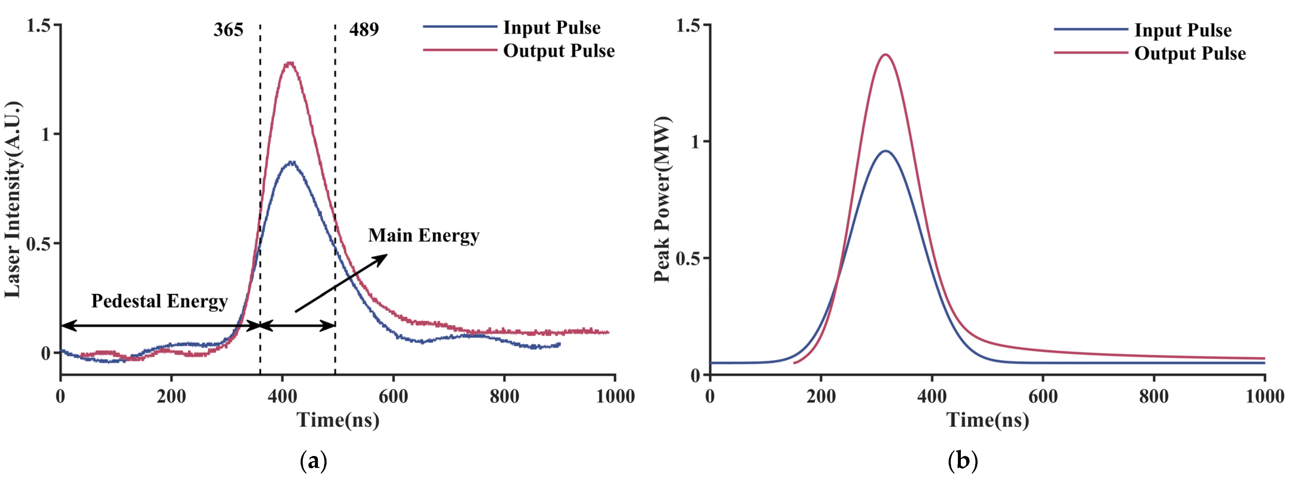
4.1. Analysis of Pulse Waveform and Gain Characteristics in High-Pressure CO₂ Oscillator–Amplifier Systems

Based on the high-pressure CO₂ six-temperature model, discharge conditions, and gas parameters, theoretical calculations were performed to determine the peak power of the laser pulse and simulate its waveform. Figure 4 presents both the experimental results and theoretical predictions of the pulse waveform changes before and after amplification, under conditions where the oscillator operates at 7 atm and the amplifier at 3 atm.

By comparing the input and output pulse waveforms, and aligning them at their peak values, the power amplification process in the amplifier can be analyzed visually. As illustrated in Figure 4, for most spectral lines, the amplifier’s power amplification predominantly occurred in the main pulse region, with limited amplification in the baseline region. During a single traveling-wave amplification process, the laser power increased from 0.88 MW to 1.33 MW. The change in the laser pulse width before and after amplification was minimal, with the measured pulse width approximately 124 ns. However, the power in the tail region of the amplified pulse exceeded that of the seed pulse, a phenomenon closely linked to the relaxation characteristics of the amplifier’s gain. Furthermore, the simulated waveform accurately represents the pulse amplification process, with both the power and pulse width closely matching the experimental results.

Based on the experimental results, a noticeable difference in the laser pulse width before and after amplification was observed across certain wavelength ranges, exhibiting a “strong–wide, weak–narrow” phenomenon. Specifically, when the laser was tuned to the “weak-line” region, the pulse width after single-pass amplification became narrower compared to the seed laser pulse. In contrast, when the laser was tuned to the “strong-line” region, the pulse width after amplification broadened significantly.

To further investigate the underlying physical mechanisms behind this phenomenon, the amplifier gain coefficient as a function of time was theoretically calculated for the wavelengths corresponding to the “strong-line” and “weak-line” regions, both before and after amplification. Based on the energy level diagram of CO₂, N₂, and CO molecules, and relevant references [16], the time evolution of the energy densities in three different CO₂, N₂, and CO vibrational modes is described using the Landau–Teller equations, which are solved numerically.

Each vibrational mode was in a steady state when there was no input light intensity (I_in(t) = 0), which allowed for the determination of the boundary conditions for the numerical calculations. Specifically, the time derivative of each vibrational mode’s energy was zero, which can be expressed as follows:

$${\displaystyle \frac{d{E}_1}{dt}}={\displaystyle \frac{d{E}_2}{dt}}={\displaystyle \frac{d{E}_3}{dt}}={\displaystyle \frac{d{E}_4}{dt}}={\displaystyle \frac{d{E}_5}{dt}}={\displaystyle \frac{dE}{dt}}=0$$

(1)

The system of equations was solved using the fourth-order Runge–Kutta numerical method. After obtaining the solutions for the energy of each vibrational mode, the results were converted into equivalent vibrational temperatures. These temperatures were then used to calculate the laser transition linewidths and the inverted particle number density. The formula for the amplifier’s small-signal gain is as follows [14]:

$$\mathrm{G}\mathrm{a}\mathrm{i}\mathrm{n}=\mathsf{\Delta }N·{\displaystyle \frac{A_{21}{c}^2}{8\pi {\nu }_0^2}}\mathrm{g}(\nu ,{\nu }_0)$$

(2)

where A₂₁ is the spontaneous emission coefficient, ν is the radiation frequency, ν₀ is the central frequency of the spectral line, g(ν,ν₀) is the normalized line shape function, and ΔN represents the population inversion between the upper and lower laser levels. The calculation formula is as follows:

$$\mathsf{\Delta }\mathrm{N}=N_{001}P(J(001))-{\displaystyle \frac{2J+1}{2J+3}}{N}_{100}P(J+1)$$

(3)

where N₁₀₀ and N₀₀₁ are the particle number densities of the upper and lower energy levels, respectively. The rotational distribution function is given by the following equation:

$$P(J(001))={\displaystyle \frac{2hc{B}_{C{O}_2}}{kT}}(2J+1)exp(-{\displaystyle \frac{hc{B}_{C{O}_2}J(J+1)}{kT}})$$

(4)

where B_CO2 represents the rotational constant of the CO₂ molecule, c is the speed of light, h is Planck’s constant, k is Boltzmann’s constant, and T denotes the gas temperature. J(001) refers to the rotational quantum number.

Since pure vibrational transition lines do not exist in CO₂ molecules, the entire molecule simultaneously occupies a specific rotational state within a given vibrational mode. Therefore, the rotational quantum number J is introduced to characterize the rotational energy levels. For example, P(20) indicates that the rotational quantum numbers of the upper and lower energy levels during the laser transition are 19 and 20, respectively.

Table 2. Parameter table for simulation calculations.

Parameter Description	Notation	Value	Units
CO2 symmetric excited level wave number	v1/c	1337	cm−1
CO2 bending excited level wave number	v2/c	667	cm−1
CO2 asymmetric excited level wave number	v3/c	2349	cm−1
N2 excited level wave number	v4/c	2330	cm−1
CO excited level wave number	v5/c	2150	cm−1
Planck’s constant	h	6.626 × 10−34	J·s
Speed of light	c	2.998 × 108	m/s
Boltzmann constant	k	1.38 × 10−23	J/K
Rotational constant	BCO2	0.3871	cm−1
Collision cross section of CO2 molecules	QCO2	1.3 × 10−18	m2
Collision cross section of N2 molecules	QN2	1.14 × 10−18	m2
Collision cross section of He molecules	QHe	3.7 × 10−19	m2
Collision cross section of CO molecules	QCO	1.14 × 10−18	m2
CO2 symmetric excitation rate	X1	5 × 10−15	m3/s
CO2 bending excitation rate	X2	3 × 10−15	m3/s
CO2 asymmetric excitation rate	X3	8 × 10−15	m3/s
N2 excitation rate	X4	2.3 × 10−14	m3/s
CO excitation rate	X5	3 × 10−14	m3/s

presents the parameters required for numerical simulations.

Based on the above formula, we calculated the small-signal gain for the 10P(20) and 10P(32) spectral lines and simulated the laser pulse waveforms before and after amplification to investigate the influence of different gain levels on the temporal waveform of the laser pulses. The corresponding results are presented in Figure 5 and Figure 6.

Figure 5 shows the simulation results for the “strong-line” 10P(20) spectral line. It can be observed that the amplifier exhibited a higher peak gain at the “strong-line” region, with a steeper rise time and a shorter relaxation time. When the amplifier was excited, the cavity rapidly gained amplification within the same time frame, reaching peak gain in a very short period. During this process, the amplifier linearly amplified different parts of the input pulse waveform, meaning both the baseline and peak portions of the incident seed light were amplified simultaneously. As a result, when measuring the laser pulse width, the “waist” of the light pulse—i.e., the width at half-maximum—expanded. The calculations show that the original pulse width of the seed light was 96 ns, increasing to 107.85 ns after single-pass amplification. These results indicate that the laser energy distribution in the time domain became broader after amplification at the strong line, leading to a decrease in energy concentration.

Figure 6 shows the simulation results for the “weak-line” 10P(10) spectral line. It can be observed that the amplifier exhibited a smaller peak gain at the “weak-line” region, with a more gradual rise time and a relatively longer relaxation time. When the amplifier was triggered, the cavity established gain more slowly within the same time frame, taking a certain amount of time to reach peak gain. This means that the seed light did not immediately undergo power amplification upon entering the cavity; only the peak portion near the upper end was amplified. As a result, when measuring the laser pulse width, the width at half-maximum of the light pulse actually decreased. The calculations show that the original pulse width of the seed light was 132 ns, decreasing to 110 ns after single-pass amplification. In this case, the laser energy distribution in the time domain became narrower, thereby increasing the energy concentration, although the laser peak power was lower compared to that at the “strong-line” region.

To provide a more detailed explanation of the temporal characteristics of amplifier gain and to account for the impact of gain saturation on the temporal waveform, we calculated the saturated laser gain. The formula for calculating the saturated gain is as follows:

$$G_s={\displaystyle \frac{G_0}{1+\frac{I}{I_s}}}$$

(5)

where G₀ is the small-signal gain, I is the laser intensity, and I_s is the saturation intensity, which can be calculated using the follow equation:

$$I_s={\displaystyle \frac{h\nu }{\sigma \tau }}$$

(6)

where h is Planck’s constant, $\nu$ is the center frequency of different spectral lines, $\tau$ is the lifetime of the upper energy state, and $\sigma$ represents the stimulated emission cross section. The calculation formula is as follows:

$$\sigma (\nu ,{\nu }_0)={\displaystyle \frac{A_{21}{c}^2}{8\pi {\nu }_0^2}}\mathrm{g}(\nu ,{\nu }_0)$$

(7)

The detailed meanings of the parameters are provided in the explanation of Equation (2). Based on the calculations, the results show that the saturated gain for the strong emission line 10P(20) was 1.683% cm⁻¹, while for the weak emission line, it was 1.421% cm⁻¹. During the amplification process of the 10P(20) laser line, the gain indeed reached saturation. To analyze the effect of saturated gain on the power amplification process, we performed a simulation to calculate the variation in amplifier gain relative to the seed laser pulse power, as illustrated in Figure 7. The saturated gain values at both spectral lines are explicitly labeled in the figure.

The blue curve in the figure represents the gain variation in the strong-line 10P(20) spectral line relative to the seed laser pulse power. The gain evolution can be divided into three stages. In the first stage, as the incident laser power increased, the amplifier gain rose rapidly, approaching the saturation threshold at 0.6 MW. This corresponds to the temporal process shown in Figure 5. The growth phase was very brief (around 70 ns), meaning the energy amplification of the pulse laser’s leading edge was insufficient. In the second stage, as the laser power increased from 0.6 MW to 1 MW, the laser gain gradually approached saturation. This stage saw a substantial gain increase, exceeding 1.5% cm⁻¹, corresponding to the effective amplification of the main laser pulse, with a duration of approximately 200–250 ns. In the third stage, once the laser gain reached saturation, stimulated emission reduced the population inversion, causing a rapid decrease in small-signal gain. However, because the saturation threshold was high, the baseline energy at the trailing edge of the pulse was effectively amplified, a process that may last over 200 ns. As a result, the waveform in the time domain shows a pulse width after amplification that is broader than the original.

The orange curve in the figure represents the gain variation of the weak-line 10P(10) spectral line relative to the seed laser pulse power, which can similarly be analyzed in three stages. In the first stage, as the laser power increased from 0 MW to 0.4 MW, the amplifier gain increased gradually. This stage lasted about 100 ns, as shown in the temporal waveform of Figure 6, during which the laser pulse was not effectively amplified. In the second stage, as the laser power increased from 0.4 MW to 1 MW, the gain growth rate accelerated, rising from 0.38% cm⁻¹ to 1.37% cm⁻¹, with an effective amplification of the laser pulse. This phase lasted approximately 200 ns, and because the gain peak was smaller than that for the strong-line region, the peak laser power after amplification was also lower. In the third stage, after effective gain extraction, the laser gain decreased. Although the decrease was slower compared to the strong-line region, the lower gain peak means that the baseline energy of the pulse’s trailing edge was not effectively amplified. Thus, the waveform in the time domain only shows effective amplification of the main pulse, resulting in a pulse width after amplification that is narrower than the original.

4.2. Limitations of the High-Pressure CO₂ Six-Temperature Model

A numerical simulation was performed using the high-pressure CO₂ six-temperature model with the Runge–Kutta method. However, various factors may have contributed to discrepancies between the simulation results and the actual outcomes. In the numerical method, we employed the fourth-order Runge–Kutta method with a step size of 10,000. According to the relevant literature, this method may have limited precision, which may introduce errors and affect the accuracy of the results [17]. Additionally, model inaccuracies may exist in simulating the laser system. In our calculations, we primarily considered an idealized environment and did not account for various cavity losses that may occur in actual experimental conditions. Furthermore, factors such as gas dissociation and circuit aging could introduce additional discrepancies. As a result, the computed values may be higher than those observed in practice [18].

These errors could lead to some deviation in the temporal waveform analysis of the nanosecond laser pulse compared to the experimental results. However, the method used here effectively describes the CO₂ multi-frequency dynamic process, and the trends in laser power, gain, and saturation are well-captured. This is evident from the comparison of the experimentally measured and numerically simulated laser waveforms in Figure 2. Therefore, the description based on the simulation results remains both scientifically valid and effective.

5. Conclusions

This study systematically investigated the temporal characteristics of CO₂ laser amplification under tunable spectral lines based on a high-pressure CO₂ MOPA system. The results reveal significant variations in both energy and pulse width before and after amplification as a function of the tuning wavelength.

In terms of laser energy, the amplification effect was significantly stronger at “strong lines” compared to “weak lines”, achieving a maximum single-pass energy amplification factor of 2.16 across the spectral bandwidth, corresponding to a small-signal gain of 1.28% cm⁻¹. Regarding the pulse width, CO₂ laser pulses at certain strong spectral lines exhibited broadening after amplification, while at some weak spectral lines, a pulse compression effect was observed. Through small-signal gain calculations and pulse waveform simulations, it was found that this phenomenon primarily arose from differences in gain build-up time at different spectral lines, which in turn influenced the amplification mechanisms of various pulse components.

The findings of this study provide important insights for the temporal optimization of narrow-pulse CO₂ lasers. Future work will focus on the temporal evolution and pulse shaping of CO₂ lasers in multi-stage amplification processes to achieve the efficient generation of high-quality narrow-pulse CO₂ lasers. These advancements will offer critical technical support for applications in extreme ultraviolet (EUV) light sources and laser isotope separation.

References

1. Laptev, V.B.; Pigul’skii, S.V. Efficient two-stage laser enrichment up to 99% of carbon-13 isotope by IR multiphoton dissociation of Freon molecules. Quantum Electron. 2022, 52, 371. [Google Scholar]
2. Makarov, G.N.; Petin, A.N. Intense infrared laser-induced radiation–collision involvement of molecules that do not absorb laser radiation in resonance with a laser field in a two-component molecular medium. JETP Lett. 2022, 115, 256–260. [Google Scholar]
3. Zhevlakov, A.P.; Seisyan, R.P.; Bespalov, V.G.; Elizarov, V.V.; Grishkanich, A.S.; Kascheev, S.V. High-efficiency bispectral laser source for EUV lithography. In Laser Applications in Microelectronic and Optoelectronic Manufacturing (LAMOM) XXI; SPIE: San Francisco, CA, USA, 2016; Volume 9735, pp. 255–264. [Google Scholar]
4. Amano, R.; Dinh, T.H.; Sasanuma, A.; Arai, G.; Hara, H.; Fujii, Y.; Hatano, T.; Ejima, T.; Jiang, W.; Sunahara, A.; et al. Influence of short pulse duration of carbon dioxide lasers on extreme ultraviolet emission from laser-produced plasmas. Jpn. J. Appl. Phys. 2018, 57, 070311. [Google Scholar]
5. Parvin, P.; Sajad, B.; Silakhori, K.; Hooshvar, M.; Zamanipour, Z. Molecular laser isotope separation versus atomic vapor laser isotope separation. Prog. Nucl. Energy 2004, 44, 331–345. [Google Scholar] [CrossRef]
6. Snyder, R. A proliferation assessment of third generation laser uranium enrichment technology. Sci. Glob. Secur. 2016, 24, 68–91. [Google Scholar]
7. Versolato, O.O.; Sheil, J.; Witte, S.; Ubachs, W.; Hoekstra, R. Microdroplet-tin plasma sources of EUV radiation driven by solid-state lasers (Topical Review). J. Opt. 2022, 24, 054014. [Google Scholar] [CrossRef]
8. Schafgans, A.A.; Brown, D.J.; Fomenkov, I.V.; Sandstrom, R.; Ershov, A.; Vaschenko, G.; Rafac, R.; Purvis, M.; Rokitski, S.; Tao, Y.; et al. Performance optimization of MOPA pre-pulse LPP light source. In Extreme Ultraviolet (EUV) Lithography VI.; SPIE: San Jose, CA, USA, 2015; Volume 9422, pp. 56–66. [Google Scholar]
9. Welch, E.; Matteo, D.; Tochitsky, S.; Joshi, C. Generating quasi-single multi-terawatt picosecond pulses in the Neptune CO2 laser system. In IEEE Advanced Accelerator Concepts Workshop (AAC); IEEE: Piscataway, NJ, USA, 2018; pp. 1–4. [Google Scholar]
10. Tochitsky, S.Y.; Narang, R.; Filip, C.; Clayton, C.E.; Marsh, K.A.; Joshi, C. Generation of 160-ps terawatt-power CO2 laser pulses. Opt. Lett. 1999, 24, 1717–1719. [Google Scholar] [PubMed]
11. Haberberger, D.; Tochitsky, S.; Joshi, C. Fifteen terawatt picosecond CO2 laser system. Opt. Express. 2010, 18, 17865–17875. [Google Scholar] [PubMed]
12. Polyanskiy, M.N.; Pogorelsky, I.V.; Babzien, M.; Palmer, M.A. Demonstration of a 2 ps, 5 TW peak power, long-wave infrared laser based on chirped-pulse amplification with mixed-isotope CO2 amplifiers. OSA Contin. 2020, 3, 459–472. [Google Scholar]
13. Feldman, B.J. Multiline short pulse amplification and compression in high gain CO2 laser amplifiers. Opt. Commun. 1975, 14, 13–16. [Google Scholar]
14. Zhang, R.; Pan, Q.; Guo, J.; Chen, F.; Yu, D.; Sun, J.; Zhang, K.; Zhang, L. Theoretical and experimental study of nanosecond pulse amplification in a CW CO2 amplifier. Infrared Phys. Technol. 2020, 111, 103537. [Google Scholar]
15. Ye, J.; Zhu, Z.; Lu, Y.; Bai, J.; Su, X.; Tan, R.; Zheng, Y. Investigation of the multi-spectral line output characteristics of a multi-atmospheric CO2 pulsed laser. Opt. Eng. 2023, 62, 056102. [Google Scholar] [CrossRef]
16. Torabi, R.; Saghafifar, H.; Koushki, A.M.; Ganjovi, A.A. Simulation and initial experiments of a high power pulsed TEA CO2 laser. Phys. Scr. 2015, 91, 015501. [Google Scholar]
17. Butcher, J.C. A history of Runge-Kutta methods. Appl. Numer. Math. 1996, 20, 247–260. [Google Scholar]
18. Torabi, R.; Silakhori, K. Generalization of the 6-Temperature model for simulation of super-atmospheric pulsed CO2 lasers output. Phys. Scr. 2021, 96, 085402. [Google Scholar] [CrossRef]
Figure 1. Setup of the high-pressure CO2 master oscillator power amplifier system.
Photonics 12 00346 g001
Figure 2. Energy amplification measurement results of high-pressure CO2 oscillator–amplifier systems: (a) 9R branch; (b) 9P branch; (c) 10R branch; (d) 10P branch.
Photonics 12 00346 g002
Figure 3. Change in pulse width relative to the original pulse width after amplification in the high-pressure CO2 oscillator–amplifier system: (a) 9R branch; (b) 9P branch; (c) 10R branch; (d) 10P branch.
Photonics 12 00346 g003
Figure 4. Pulse waveforms of the 10R(28) spectral line before and after amplification in the high-pressure CO2 oscillator–amplifier system: (a) experimental results; (b) simulation results.
Photonics 12 00346 g004
Figure 5. Simulation results of pulse width and gain for 10P(20) before and after amplification in high-pressure CO2 oscillator–amplifier systems.
Photonics 12 00346 g005
Figure 6. Simulation results of pulse width and gain for 10P(10) before and after amplification in high-pressure CO2 oscillator–amplifier systems.
Photonics 12 00346 g006
Figure 7. Numerical calculation results of gain variation for spectral lines 10P(20) and 10P(10) with incident laser power.
Photonics 12 00346 g007