Optical Field-to-Field Translation Under Atmospheric Turbulence: A Conditional GAN Framework with Embedded Turbulence Parameters

Abstract

We propose a field mapping approach for the propagation of laser beams through atmospheric turbulence, leveraging a Generative Adversarial Network (GAN). The proposed GAN utilizes a U-Net architecture as its generator, with turbulence characteristic parameters introduced into the bottleneck layer of the U-Net network, enabling effective control over the generator. This design allows for the flexible simulation of Gaussian beam propagation across a range of turbulence intensities and transmission distances. A comparative analysis between the neural network predictions and numerical simulation results indicates that the neural network can achieve a field mapping speedup of four orders of magnitude while maintaining a relative error within 16% for the second-order statistical moments of the light spot. Additionally, the study investigates the effect of varying turbulence intensities on prediction accuracy. The results indicate that high-frequency speckle patterns caused by beam breakup are the primary factor limiting prediction accuracy under strong or saturated turbulence conditions.

1. Introduction

When a laser beam propagates through the atmosphere, it is significantly influenced by small temperature fluctuations, as well as wind shear and turbulence. These factors lead to irregular distributions of the refractive index in both space and time, resulting in the distortion of the laser wavefront. Consequently, this distortion degrades the coherence of the laser, causes dissipation of laser energy and significantly impacts the transmission efficiency of the laser [1,2,3,4]. Specifically, atmospheric turbulence can cause several detrimental effects on laser communication:

Beam Spread: Atmospheric turbulence causes the laser beam to spread out as it propagates, leading to a larger spot size at the receiver and reduced signal intensity [1,2].

Beam Wander: The random variations in the refractive index cause the laser beam to wander off its intended path, making it difficult for the receiver to maintain alignment and track the beam accurately [1,2].

Angle-of-Arrival Fluctuations: The angle at which the laser beam arrives at the receiver fluctuates due to turbulence, complicating the task of maintaining optimal alignment and reducing the efficiency of signal reception [1,2].

Scintillation: The intensity of the laser beam fluctuates randomly as it propagates through the turbulent atmosphere, leading to signal fading and increased error rates [1,2].

Phase Distortion: Turbulence induces random phase changes in the laser beam, which can degrade the performance of coherent communication systems by reducing the mixing efficiency and increasing error rates [1,2].

Currently, the random phase screen method, based on wave theory, is commonly used to simulate laser beam propagation in a turbulent atmosphere [5,6]. It models the continuous medium along the laser path as discrete phase screens and treats the optical-field propagation between them as vacuum diffraction. Specifically, before reaching each screen, the optical field undergoes vacuum diffraction and is then modulated by phase screens. Iterating this process in a sequential manner can efficiently simulate the laser beam propagation in turbulent media.

The key steps in this numerical simulation encompass the computation of phase screens and the diffraction of the optical field. For the diffraction calculation, it is typically addressed by the split-step method based on the Fresnel diffraction in angular spectrum form, which has become a well-established approach in numerical diffraction computations [7]. Regarding the phase screen calculation, the power-spectrum inversion algorithm is widely utilized to generate phase screens [8,9,10]. Considering its substantial influence on the simulation results, a great deal of research has been conducted to enhance computational efficiency without compromising accuracy, including sparse spectrum technology introduced by Charnotskii [11,12], random subharmonic sampling by Paulson [13] and the sinc series approximation based method introduced by Cubillos [14]. Additionally, the authors have proposed a phase screen generation technique based on sampling optimization [15,16]. All these methods are aimed at improving the speed and precision of phase screen generation by sampling the refractive index spectrum.

Despite these advancements, several challenges persist. Even though remarkable improvements have been made in numerical simulation efficiency, achieving real-time applicability is still extremely difficult. This is mainly attributed to two key factors. Firstly, each transmission calculation involves multiple iterations of diffraction and modulation processes, which are inherently time-consuming operations. Secondly, given the stochasticity of atmospheric turbulence, obtaining the necessary optical field statistics demands statistical analysis of a large number of samples. Typically, this can only be accomplished through ensemble average. These challenges are deeply rooted in the numerical computation approach, indicating that mere algorithmic improvements are insufficient to significantly enhance the simulation speed.

Fortunately, recent breakthroughs in artificial intelligence, specifically generative AI, present promising solutions for these challenges. In the realm of image generation, generative AI has exhibited remarkable progress. It has evolved from variational autoencoders [17] and Generative Adversarial Networks [18,19] (GANs) to the state-of-the-art diffusion models [20], which have substantially enhanced both image quality and content control. In our study, taking the initial optical field distribution as input and atmospheric turbulence conditions as control parameters, generative AI can generate the atmospheric-turbulence-altered intensity distribution on the received plane.

Among the aforementioned generative AI frameworks, GANs stand out for their rapid output capabilities, generating the intensity distribution of laser transmission through atmospheric turbulence more efficiently than diffusion models, which require multiple denoising steps. By avoiding the blurring issues associated with variational autoencoders, GANs are particularly well-suited for the fast field mapping of laser transmission in a turbulent atmosphere. Recent research has demonstrated the effectiveness of GANs in mitigating turbulence-induced degradation. For underwater scenarios, Chen et al. proposed a deep-learning-based method to reconstruct images degraded by ocean turbulence [21]. Their approach employed a power spectrum inversion method to simulate turbulence phase screens, generating degraded images under varying turbulence conditions. A Pix2Pix-based network was then trained to recover the original images, achieving high-fidelity reconstruction, though performance degraded with increasing turbulence strength and propagation distance. Meanwhile, for atmospheric turbulence, Rai et al. addressed the challenge of mixed distortions (geometric warping and blurring) by introducing a two-stage adversarial network (DT-GAN+ and DTD-GAN+) [22]. Their approach outperforms the general state-of-the-art image-to-image translation models and baseline restoration models. In contrast to these inverse reconstruction approaches, our work addresses the forward modeling problem—simulating how laser beams become distorted when propagating through atmospheric turbulence. While existing studies focus on removing turbulence effects from degraded signals, we propose a GAN-based architecture that directly generates intensity distributions of turbulence-distorted laser beams. This forward-simulation capability provides a computationally efficient alternative to traditional numerical methods like the random phase screen method.

2. Network Design

2.1. The Laser Beam Model

The goal of the proposed model is to simulate the intensity distribution of a laser beam after propagating through turbulent atmospheres. The input to the model is the optical field distribution at the source plane, and the output is the intensity distribution on the receiving plane, while the transmission distance and the refractive index structure constant are provided as additional control parameters in the bottleneck layer.

The mathematical model for laser beam propagation in a turbulent atmospheres is based on the split-step method using Fresnel diffraction in angular spectrum form [6,23]. The propagation process can be expressed as follows:

$$\begin{array}{cc}\hfill U_n({\mathbf{r}}_n,z_n)& =Q[{\displaystyle \frac{m_{n-1}-1}{m_{n-1}{z}_{n-1}}},{\mathbf{r}}_n]\hfill \\ \hfill & \times \prod _{i=1}^{n-1}\left\{T[z_i,z_{i+1}]F^{-1}[{\mathbf{f}}_i,{\displaystyle \frac{{\mathbf{r}}_{i+1}}{m_i}}]Q[{\displaystyle \frac{4{\pi }^2{z}_i}{m_{i}k}},{\mathbf{f}}_i]F[{\mathbf{r}}_i,{\mathbf{f}}_i]{\displaystyle \frac{1}{m_i}}\right\}\hfill \\ \hfill & \times \left\{Q[{\displaystyle \frac{1-m_1}{z_1}},{\mathbf{r}}_0]T[z_0,z_i]U_0\left({\mathbf{r}}_0,0\right)\right\},\hfill \end{array}$$

(1)

where $U_0({\mathbf{r}}_1,0)$ is the spatial distribution of the optical field at the source plane. m serves as the scaling parameter that controls the spatial sampling interval on the receiving plane, which helps accommodate the beam width increase caused by turbulence and diffraction effects. Q, F, $F^{-1}$ and T are a set of operators. Specifically, Q represents the second-order phase factor, F represents the Fourier Transform, $F^{-1}$ represents the Inverse Fourier Transform and T represents the phase modulation induced by turbulence. They are defined as follows:

$$Q\left[c,\mathbf{r}\right]\left\{U\left(\mathbf{r}\right)\right\}\equiv e^{{\displaystyle \frac{ikc}{2}}{\left|\mathbf{r}\right|}^2}U\left(\mathbf{r}\right),$$

(2)

$$F[\mathbf{r},\mathbf{f}]\left\{U\left(\mathbf{r}\right)\right\}\equiv \underset{-\infty }{\overset{\infty }{\int }}U\left(\mathbf{r}\right)e^{-i2\pi \mathbf{f}·\mathbf{r}}d\mathbf{r},$$

(3)

$$F^{-1}[\mathbf{f},\mathbf{r}]\left\{U\left(\mathbf{f}\right)\right\}\equiv \underset{-\infty }{\overset{\infty }{\int }}U\left(\mathbf{f}\right)e^{i2\pi \mathbf{f}·\mathbf{r}}d\mathbf{f},$$

(4)

$$T[z_i,z_{i+1}]=e^{-i\varphi \left({\mathbf{r}}_{\mathbf{i}+\mathbf{1}}\right)},$$

(5)

where $\varphi \left(r_{i+1}\right)$ represents the phase screen that can be calculated via phase screen generation method based on spectral inversion:

$$\begin{array}{cc}\hfill \phi (x,y)& ={\sum }_{f_x}{\sum }_{f_y}\mathbf{h}(f_x,f_y)\sqrt[]{{\Phi }_{\phi }(f_x,f_y)}\hfill \\ \hfill & \times exp\left[j(f_{x}x+f_{y}y)\right]\Delta f_x\Delta f_y.\hfill \end{array}$$

(6)

In Equation (6), $\mathbf{h}(f_x,f_y)$ represents a complex Hermitian Gaussian random matrix with zero mean and unit variance. ${\Phi }_{\phi }(f_x,f_y)$ denotes the power spectral density function that conforms to the atmospheric turbulence spectrum. $f_x$ and $f_y$ are the spatial frequencies in the x direction and y direction, respectively. The power spectral density function that follows the von Karman spectrum can be expressed as follows:

$${\Phi }_{\phi }(f_x,f_y)=0.023r_0^{-5/3}{[{\left(2\pi f\right)}^2+k_0^2]}^{-11/6}{e}^{-{\displaystyle \frac{{\left(2\pi f\right)}^2}{k_m^2}}},$$

(7)

where $k_m=5.92/l_0$, $k_0=2\pi /L_0$ and $l_0$ and $L_0$ represent the inner scale and the outer scale, respectively. $r_0$ represents the atmospheric coherence length, also known as the Fried parameter [1]. It is related to the refractive index structure constant $C_n^2$ and the propagation distance z as follows:

$$r_0={[0.423k^2·sec\left(z\right)·{\int }_0^h{C}_n^2\left(h\right)dh]}^{-3/5},$$

(8)

Specifically, when the laser beam propagates in a horizontal path, the $r_0$ can be expressed as follows:

$$r_0={\left(0.423k^2{C}_n^{2}z\right)}^{-3/5}.$$

(9)

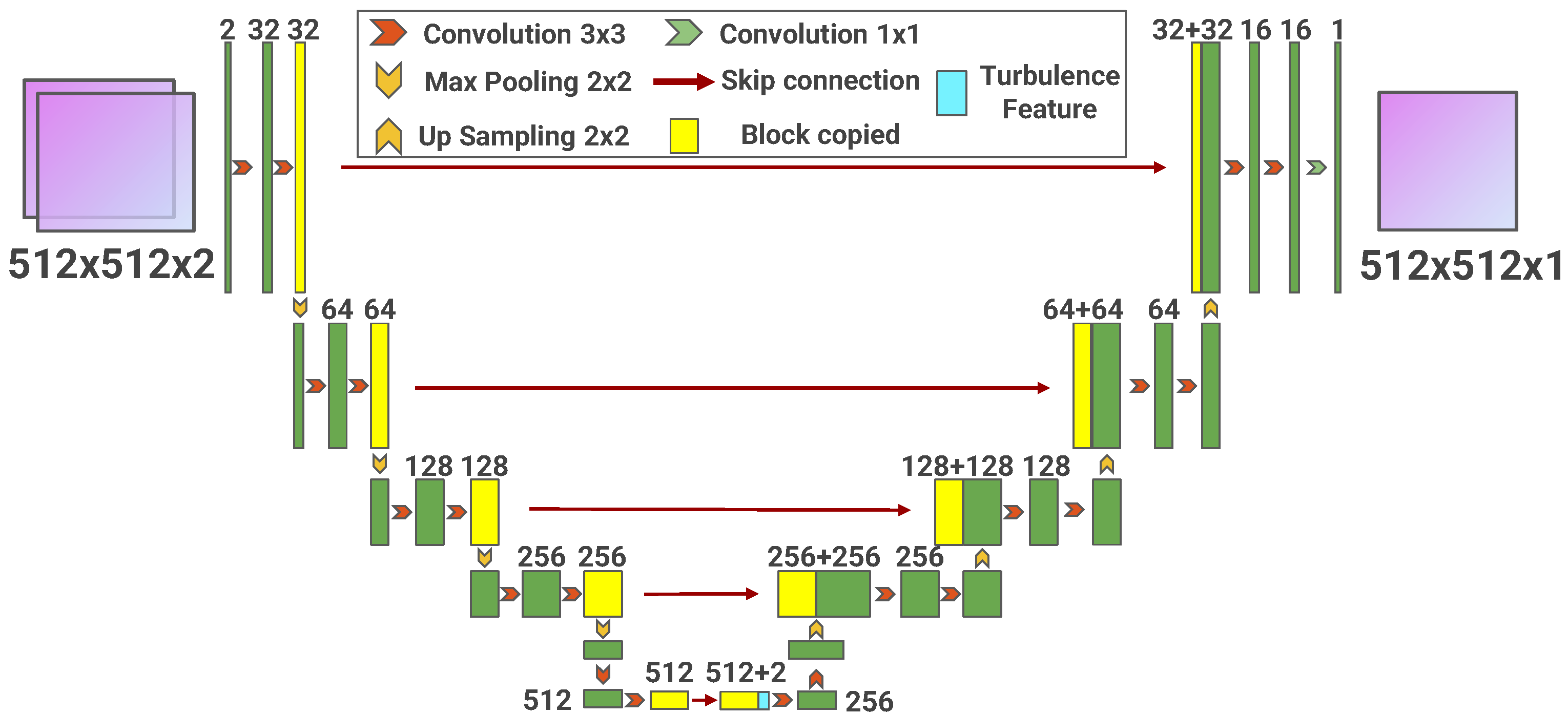
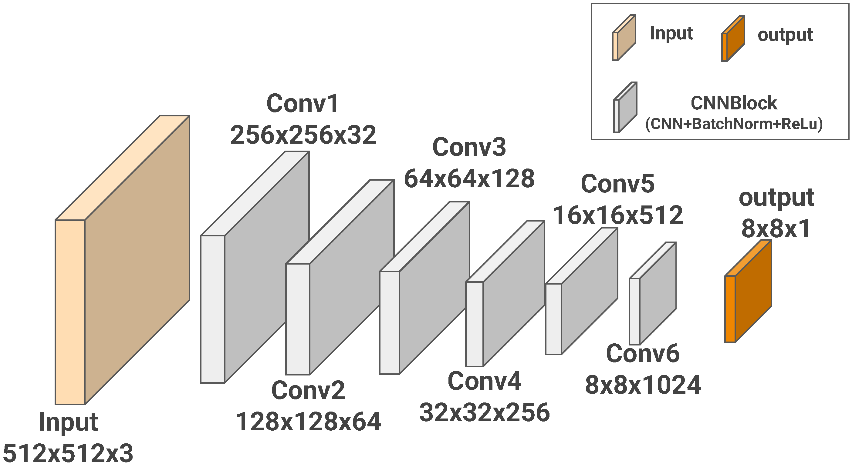
2.2. Proposed GAN Architecture

By analyzing the calculation process of the above-mentioned model, it can be deduced that to complete the calculation of laser beam propagation in a turbulent atmosphere, it is essential to feed the source-plane optical-field distribution, transmission distance z and refractive index structure constant $C_n^2$ into the calculation model as inputs, and the final output is the optical-field distribution on the receiving plane. To simulate this process efficiently, we propose a GAN-based architecture. The generator, based on the U-Net [24] network, takes the source-plane optical field distribution as input and outputs the intensity distribution on the receiving plane. The discriminator, based on the PatchGAN network [25], evaluates the quality of the generated samples. The structure of the U-Net generator is shown in Figure 1.

As depicted in Figure 1, the U-Net network essentially adopts an encoder–decoder architecture. The left-hand side of the network progressively abstracts the input optical-field distribution, extracting deep-level features at the middle layer. Subsequently, through the decoding process on the right-hand side, it reconstructs an output optical-field distribution with the same size as the input. Considering that most statistical analyses of atmospheric turbulence predominantly rely on the intensity distribution, the optical-field distribution is replaced by the intensity distribution.

During the GAN training process, a discriminator is necessary to assess the quality of the generated samples. In this study, PatchGAN is used as a discriminator, as it has been proven effective in similar tasks according to previous research [19,26]. The architecture of the PatchGAN network is illustrated in Figure 2.

3. Training Data and Network Training

The training sample was prepared via the numerical simulation method mentioned above. Based on the network architecture, the inputs for the U-Net network are defined as the initial optical field distribution (comprising the amplitude distribution and phase distribution) and the control condition parameters (including the refractive index structure constant and transmission distance).

The initial optical field distribution follows a fundamental-mode Gaussian distribution. The initial phase distribution varies depending on the collimation and focusing state of the beam. To match the dimensionality of the middle layer of the U-Net network, the characteristic parameters of the intensity of the turbulence are expanded in dimension to form a characteristic layer (with dimensions of 16 × 16 × 2). Here, the third dimension represents different control condition parameters. Finally, this characteristic layer is concatenated with the feature layer along the third dimension.

As for the PatchGAN network, its inputs consist of the initial optical field distribution and the intensity distribution of the receiving plane. The intensity distribution output of the U-Net network is labeled as “fake”, while the intensity distribution obtained through numerical simulation is labeled “true”.

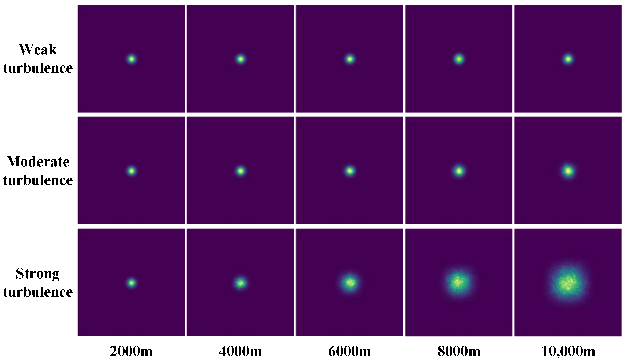
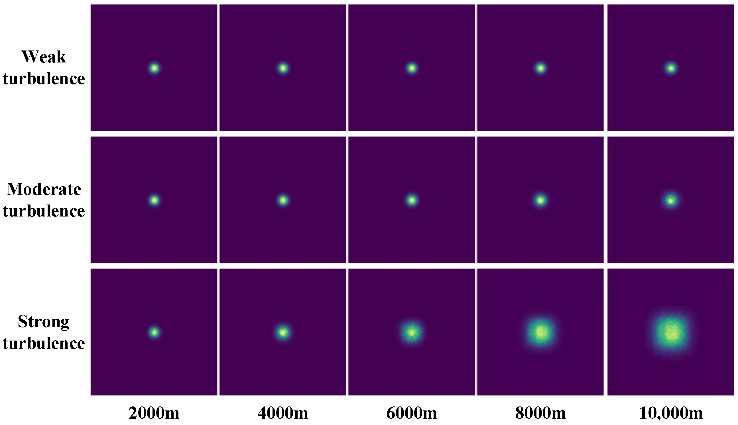
3.1. Building the Training Dataset

The parameters of the training sample set are presented as follows:

• The input optical field is a fundamental-mode Gaussian beam with a beam waist radius of 0.1 m and a wavelength of 1.08 μm. This Gaussian beam can be in a collimated or focused state. In the focused state, the focal length is set equal to the corresponding transmission distance;
• Regarding the turbulence-related parameters, the refractive index structure constant is linearly sampled 100 times from $1\times {10}^{-16}$ to $1\times {10}^{-13}$${\mathrm{m}}^{-2/3}$. The outer scale parameter is 100 m, and the inner scale parameter is 0.01 m. The number of phase screens on the transmission path is set to 20;
• For the receiving-plane and transmission parameters, the physical dimension of the receiving plane is $1\mathrm{m}\times 1\mathrm{m}$. The transmission distance ranges from 0 to 10,000 m, with a linear separation of 200 m intervals.

The above-mentioned parameters are substituted into the numerical model based on the random phase screen method to calculate the intensity distribution of the receiving plane. Considering the stochasticity of the atmospheric turbulence, the calculations are repeated 400 times for each set of parameters, and the average result is used as the label data for the network.

The dataset is designed primarily for terrestrial laser communication scenarios. The refractive index structure constant ($C_n^2$) is linearly sampled across three orders of magnitude (${10}^{-16}$ to ${10}^{-13}{\mathrm{m}}^{-2/3}$) to capture weak to strong turbulence conditions, while transmission distances (0–10 km) cover the typical transmission ranges of terrestrial laser communication. The inclusion of both collimated and focused Gaussian beam configurations accounts for diverse launch conditions, with focused beams adopting focal lengths matching their transmission distances for physical consistency.

Subsequently, a training dataset consisting of 10,000 training samples is created. Each sample includes the source-plane optical field with dimensions of 512 × 512 × 2, the control-condition parameters of 16 × 16 × 2 and the label representing the intensity distribution with dimensions of 512 × 512.

3.2. Loss Function

To align the intensity distribution generated by the network with numerical simulation results, we incorporate a loss term aware of turbulence statistics into the objective function of the generator. Drawing from Andrews’ beam propagation theory [1], we select the beam wander variance (a first-order statistical moment) as our key physical metric. This choice balances mathematical tractability (ensuring gradient stability during backpropagation) and physical interpretability. The centroid displacement is computed as follows:

$$〈r_c〉=\sqrt[]{〈r_{cx}^2〉+〈r_{cy}^2〉}=\sqrt[]{{\left({\displaystyle \frac{\int \int x〈I(x,y,L)〉dxdy}{\int \int 〈I(x,y,L)〉dxdy}}\right)}^2+{\left({\displaystyle \frac{\int \int y〈I(x,y,L)〉dxdy}{\int \int 〈I(x,y,L)〉dxdy}}\right)}^2},$$

(10)

The total power of the beam in the receiving plane is the sum of the power weighted in the x direction and y direction, respectively. When the two-dimensional intensity distribution is obtained, the beam wander variance can be obtained by numerical solution, and then the $L_1$ loss of the beam wander variance can be introduced,

$$\begin{array}{cc}\hfill L_{BW}& =\sqrt[]{{\left({\displaystyle \frac{{\displaystyle \sum _{i=-N/2}^{N/2-1}}{\displaystyle \sum _{j=-N/2}^{N/2-1}}i·B_{ij}·\Delta x\Delta y}{{\displaystyle \sum _{i=-N/2}^{N/2-1}}{\displaystyle \sum _{j=-N/2}^{N/2-1}}{B}_{ij}·\Delta x\Delta y}}\right)}^2+{\left({\displaystyle \frac{{\displaystyle \sum _{i=-N/2}^{N/2-1}}{\displaystyle \sum _{j=-N/2}^{N/2-1}}j·B_{ij}·\Delta x\Delta y}{{\displaystyle \sum _{i=-N/2}^{N/2-1}}{\displaystyle \sum _{j=-N/2}^{N/2-1}}{B}_{ij}·\Delta x\Delta y}}\right)}^2}\hfill \\ \hfill & -\sqrt[]{{\left({\displaystyle \frac{{\displaystyle \sum _{i=-N/2}^{N/2-1}}{\displaystyle \sum _{j=-N/2}^{N/2-1}}i·G{\left(A\right)}_{ij}·\Delta x\Delta y}{{\displaystyle \sum _{i=-N/2}^{N/2-1}}{\displaystyle \sum _{j=-N/2}^{N/2-1}}G{\left(A\right)}_{ij}·\Delta x\Delta y}}\right)}^2+{\left({\displaystyle \frac{{\displaystyle \sum _{i=-N/2}^{N/2-1}}{\displaystyle \sum _{j=-N/2}^{N/2-1}}j·G{\left(A\right)}_{ij}·\Delta x\Delta y}{{\displaystyle \sum _{i=-N/2}^{N/2-1}}{\displaystyle \sum _{j=-N/2}^{N/2-1}}G{\left(A\right)}_{ij}·\Delta x\Delta y}}\right)}^2},\hfill \end{array}$$

(11)

In Equation (9), i and j denote the sequence numbers of the computing grid in the x and y directions, respectively. $\Delta x$ and $\Delta y$ represent the grid sizes in the x and y directions, respectively. N denotes the numbers of the computing grid. The input optical field is denoted as A, and the generator network is represented by G. Meanwhile, B serves as the label corresponding to the intensity distribution generated by numerical simulation. Based on these defined parameters, the modified loss function is formulated as follows:

$$L_G=L_{adv}+\lambda ·L_{pix}+\beta ·L_{BW}.$$

(12)

where $L_{adv}$ represents the adversarial loss calculated by the Binary Cross Entropy (BCE) loss function; $L_{pix}$ represents the pixel loss calculated by the $L_1$ loss function. For the discriminator network, we use a BCE loss function corresponding to the adversarial loss. Subsequently, the Adam optimizer is employed with the first-order moment exponential decay rate ${\beta }_1=0.05$ and the second-order moment exponential decay rate ${\beta }_2=0.999$. The hyperparameters $\lambda$ and $\beta$ are set to 5 and 0.5, respectively, based on preliminary experiments to balance the influence of different loss components and optimize the model performance.

By incorporating beam wander variance, the model explicitly enforces statistical consistency with wave propagation physics. This first-order moment constraint acts as a regularizer, preventing physically implausible solutions that might otherwise satisfy purely data-driven terms ($L_{adv}$ and $L_{pix}$). The hierarchical combination of above losses enables simultaneous correction of global mode collapse (via GAN training), local artifacts (via pixel alignment) and statistical inconsistencies (via beam wander variance).

3.3. Training Method

To address the GAN’s training challenges, a two-step training method was employed to achieve network convergence gradually. In the first step, a total of 1500 training epochs were conducted. The generator network and the discriminator network were trained alternately at a ratio of 1:1; that is, the generator network was trained once, and then the discriminator network was trained once. The labels for the discriminator network were set as follows: the real distribution was labeled as 1, and the fake distribution was labeled as 0. The learning rate of the optimizers for both the generator and discriminator networks was set to 0.001. This balanced initialization phase establishes fundamental turbulence pattern recognition while preventing early mode collapse through synchronized parameter updates. The 0.001 learning rate provides sufficient gradient momentum to escape local minima in high-dimensional phase space (≈${10}^6$ parameters), while the strict alternation prevents either network from overspecializing.

In the second step, an additional 1500 training rounds were executed. The discriminator network was first reset to its initial randomized state to disrupt local Nash equilibrium traps formed during step 1 through a controlled symmetry-breaking mechanism. The generator and discriminator then underwent alternating training at a 1:2 ratio, implementing a curriculum learning strategy that forced the generator to refine small-scale turbulence features, while granting the discriminator double gradient updates to enhance its discrimination acuity. The discriminator’s labeling scheme was inverted (real distribution marked as 0, generated distribution as 1), reshaping the loss landscape through adversarial gradient remodeling. This reverse incentive mechanism creates competing gradient directions, effectively suppressing residual mode collapse during weight updates. The learning rates of both networks were reduced to 0.0001 to ensure that the magnitudes of the parameter update aligned with Step 1.

Throughout the process, the generator maintained continuous training, preserving acquired atmospheric channel characteristics while adapting to the discriminator’s evolving discrimination interface, and the whole training process utilized an NVIDIA A100 GPU (NVIDIA Corporation, Santa Clara, CA, USA). and took 4 days to complete.

4. Results

First, we present the averaged distorted intensity distributions induced by turbulence for different turbulence intensities and transmission distances, which were predicted by the neural network and calculated through numerical simulations. The refractive index structure constant takes values of $1\times {10}^{-16}$, $1\times {10}^{-15}$ and $1\times {10}^{-14}$${\mathrm{m}}^{-2/3}$, and the transmission distances are set to 2000 m, 4000 m, 6000 m, 8000 m and 10,000 m. For each value of the refractive index structure constant, the corresponding Fried parameter and Rytov variance within the transmission distances mentioned above are shown in

Table 1. The Rytov variances and Fried parameters corresponding to various refractive index structure constants and transmission distances.

	${\mathit{C}}_{\mathit{n}}^2$ ($m^{-2/3}$)	Distance
		2000 m	4000 m	6000 m	8000 m	10,000 m
Rytov Variance ${\sigma }_R^2$	${10}^{-16}$	0.01	0.04	0.08	0.14	0.2
	${10}^{-15}$	0.1	0.38	0.81	1.37	2.06
	${10}^{-14}$	1.08	3.85	8.10	13.73	20.68
Fried Parameter $r_0$ (m)	${10}^{-16}$	0.532	0.351	0.275	0.231	0.202
	${10}^{-15}$	0.134	0.088	0.069	0.058	0.051
	${10}^{-14}$	0.033	0.022	0.017	0.014	0.013

, which represents weak, moderate and strong turbulence conditions.

Figure 3 and Figure 4 show the averaged distorted intensity distribution of collimated Gaussian beams propagating through atmospheric turbulence, which are calculated by the generator network and numerical simulation, respectively. From top to bottom, the rows in the figures represent different values of the refractive index structure constant, while from left to right, the columns correspond to different transmission distances.

The figures reveal that the intensity distribution of the laser beam predicted by the neural network aligns well with the outcomes of numerical simulations. Moreover, the radius of the laser beam exhibits an increasing trend with the growth of both transmission distance and turbulence intensity. This observation is in line with the theoretical understanding of laser beam propagation in turbulent media [27]. It strongly suggests that the neural network has effectively captured the influence of turbulence on the propagation of the laser beam.

Similarly, Figure 5 and Figure 6 illustrate the averaged distorted intensity distribution of focused Gaussian beams propagating through atmospheric turbulence, which indicate a high degree of consistency between the predictions of the neural network and the outcomes of numerical simulations. In addition, from the patterns of intensity distribution shown in Figure 6, it is clearly manifested that under weak-turbulence conditions, the focusing spot experiences negligible expansion. However, when a certain turbulence intensity is reached, the converging ability of the Gaussian beam is overshadowed by the expansion effects induced by turbulence, resulting in the formation of a significantly spread spot. This phenomenon is in line with the theory of laser beam propagation in atmospheric turbulence.

By replacing the numerical simulation approach with a neural network, we achieve a significant reduction in computation time, decreasing from 15 s to just 6 milliseconds—an impressive reduction of nearly four orders of magnitude. This substantial decrease in computational duration enables the proposed method to effectively meet the demands of applications requiring real-time performance.

To further assess the prediction accuracy of the neural network, we utilized the second moment of the intensity distribution, namely, the long-term beam radius, as an index for evaluation. A comparative analysis was conducted between the prediction results obtained from the neural network and those derived from numerical simulations, as illustrated in Figure 7 and Figure 8.

The refractive index structure constants were set to $1\times {10}^{-16}$, $1\times {10}^{-15}$, $1\times {10}^{-14}$ and $1\times {10}^{-14}{\mathrm{m}}^{-2/3}$, and the transmission distance took values from 500 to 10,000 m, with a linear separation of 500 m intervals, which represent weak, moderate, strong and saturated turbulence conditions. The corresponding Rytov variances and Fried parameters are shown in

Table 2. The Rytov variances and Fried parameters under varying conditions.

	${\mathit{C}}_{\mathit{n}}^2$ ($m^{-2/3}$)	Value Range *
Rytov Variance ${\sigma }_R^2$	${10}^{-16}$	0.001–0.207
	${10}^{-15}$	0.008–2.067
	${10}^{-14}$	0.085–20.67
	${10}^{-13}$	0.851–206.7
Fried Parameter $r_0$ (m)	${10}^{-16}$	1.222–0.202
	${10}^{-15}$	0.307–0.051
	${10}^{-14}$	0.077–0.013
	${10}^{-13}$	0.019–0.003

* Range represents variation over 0.5–10 km distance.

.

From the results of the long-term beam radius shown in Figure 7 and Figure 8, after being trained on a large-scale training set, the neural network has the ability to simulate the laser beam propagation in the atmospheric turbulent medium, and the relative error for various turbulence intensities and transmission distances does not exceed 16%.

5. Discussion

A further analysis of the results shown in Figure 7 and Figure 8 reveals that, in the case of weak turbulence, both the numerical simulation results and the neural network prediction results exhibit violent oscillations around the theoretical curve, with the overall trend being notably non-smooth. This is because the collimated Gaussian beam in the case of weak turbulence is less affected by turbulence, and its long-term beam radius changes slowly with the increase in the transmission distance. Therefore, even some minor disturbances can cause the statistical results to be magnified in the figure. However, by observing the magnitude of the error, we can see that although the results seem to oscillate violently around the theoretical curve, the relative error shows that all fluctuations are within the error range of 2%, so the actual results are in good agreement with the theoretical curve and numerical simulation results.

Secondly, it is evident that the prediction accuracy of the neural network is higher under weak to moderate turbulence conditions compared to strong and saturated turbulence conditions. This disparity can be attributed to the fragmentation of the laser beam under strong or saturated turbulence conditions, resulting in the formation of numerous small speckles within the two-dimensional intensity pattern. From the perspective of image processing, these speckles manifest as high-frequency signals. The CNN-based neural network encounters challenges in effectively extracting features associated with such high-frequency signals [28], which imposes limitations on its prediction capabilities. Consequently, the error in the neural network’s predictions of intensity distribution is greater in strong and saturated turbulence conditions than in weak and moderate turbulence conditions.

The same phenomenon can be observed in Figure 4 and Figure 6. Particularly, under the conditions of strong turbulence and a transmission distance of 10,000 m, the intensity distribution exhibits a square-like shape. The fundamental reason for this phenomenon is that the CNN-based network is unable to capture high-frequency feature information. To be more specific, it is related to the low-frequency bias and mode collapse of GANs.

• The GANs prioritize learning low-frequency global features (e.g., overall intensity distribution) while struggling to synthesize high-frequency stochastic details (e.g., sub-pixel speckle breakups).
• The square symmetry of convolutional kernels inherently biases the generator toward blocky outputs with sharp edges when high-frequency turbulence effects are underlearned, rather than producing rotationally symmetric Gaussian or random speckles.
• Strong turbulence induced speckles exhibit extreme multimodality (infinite possible spatial configurations for a given turbulence strength). When GANs cannot cover all modes, they may collapse to a “statistical average” state.
• The generator learns that regular square patterns can partially match certain global statistics (e.g., total energy conservation or pixel mean) to fool the discriminator. This strategy, though unphysical, becomes a local Nash equilibrium in adversarial training.

Finally, in the context of saturated turbulence, substantial discrepancies are observed in both numerical simulation outcomes and neural network predictions compared to theoretical expectations. Notably, once the transmission distance exceeds 5000 m, the theoretical values are significantly elevated relative to those observed in previous cases. This phenomenon primarily arises from the absence of an effective theoretical framework that accurately characterizes the propagation of laser beams under saturated turbulence conditions. The theory employed in this study is primarily designed to address general turbulence scenarios. Thus, the general turbulence theory proves inadequate for accurately modeling such conditions.

6. Conclusions

In this paper, a simulation method for laser beam propagation in a turbulent atmosphere based on GAN is proposed. Firstly, a generator based on the U-Net network and a discriminator based on the PatchGAN network are designed. In the construction of the generator, the refractive index structure constant and the transmission distance were introduced as control conditions into the bottleneck layer of the generator. A two-step adversarial training strategy was utilized to complete the training of the generator network, enabling the simulation of Gaussian beams under different turbulence conditions and different transmission distances.

Compared with the traditional numerical method, the neural network method can increase the simulation speed by four orders of magnitude. Furthermore, under various turbulence conditions, the trends of how the second-order statistical moment of the predicted outcomes changes with distance align well with those derived from numerical simulations. Additionally, the relative error is maintained within 16%.

Finally, the differences in the prediction accuracy of the neural network for different turbulence intensities were analyzed. The results show that under weak and moderate turbulence conditions, the neural network prediction results exhibit high accuracy. However, under strong and saturated turbulence conditions, the prediction accuracy of the neural network decreases. This is because the fragmentation of the laser spot leads to the inability of the neural network to effectively capture a large number of high-frequency speckles. Given the complexity of atmospheric turbulence and its potential to introduce intricate patterns, it is important to consider the balance between robustness and accuracy in our models [29,30,31]. Future research will focus on addressing these challenges to improve prediction accuracy under varying turbulence conditions.

References

1. Andrews, L.C.; Phillips, R.L. Laser Beam Propagation Through Random Media; SPIE Press: Bellingham, WA, USA, 2005. [Google Scholar]
2. Khare, K.; Lochab, P.; Senthilkumaran, P. Theory of wave propagation in a turbulent medium. In Orbital Angular Momentum States of Light; IOP Publishing: London, UK, 2020; pp. 7-1–7-39. [Google Scholar] [CrossRef]
3. Hulea, M.; Tang, X.; Ghassemlooy, Z.; Rajbhandari, S. A review on effects of the atmospheric turbulence on laser beam propagation—An analytic approach. In Proceedings of the 2016 10th International Symposium on Communication Systems, Networks and Digital Signal Processing (CSNDSP), Prague, Czech Republic, 20–22 July 2016; pp. 1–6. [Google Scholar] [CrossRef]
4. Murty, S.S.R. Laser beam propagation in atmospheric turbulence. Proc. Indian Acad. Sci. USA 1979, 2, 179–195. [Google Scholar] [CrossRef]
5. Salmanowitz, J.; Zandt, N.R.V. Phase Screen Generation for Non-Kolmogorov Turbulence. In Proceedings of the Imaging and Applied Optics Congress 2022 (3D, AOA, COSI, ISA, pcAOP), Vancouver, BC, Canada, 11–15 July 2022. [Google Scholar]
6. Frehlich, R. Simulation of laser propagation in a turbulent atmosphere. Appl. Opt. 2000, 39, 393–397. [Google Scholar] [PubMed]
7. Mcglamery, B.L. Computer Simulation Studies of Compensation of Turbulence Degraded Images. Proc. SPIE-Int. Soc. Opt. Eng. 1976, 74, 225–233. [Google Scholar]
8. Jiang, R.; Wang, K.; Tang, X.; Wang, X. Investigation of Oceanic Turbulence Random Phase Screen Generation Methods for UWOC. Photonics 2023, 10, 832. [Google Scholar] [CrossRef]
9. Yang, Z.Q.; Yang, L.; Gong, L.; Wang, L.G.; Wang, X. Waveform Distortion of Gaussian Beam in Atmospheric Turbulence Simulated by Phase Screen Method. J. Math. 2022, 2022, 5939293. [Google Scholar] [CrossRef]
10. Herman, B.J.; Strugala, L.A. Method for inclusion of low-frequency contributions in numerical representation of atmospheric turbulence. Proc. SPIE-Int. Soc. Opt. Eng. 1990, 1221, 183–192. [Google Scholar]
11. Charnotskii, M. Sparse spectrum model for a turbulent phase. J. Opt. Soc. Am. A 2013, 30, 479. [Google Scholar]
12. Charnotskii, M. Sparse spectrum model for the turbulent phase simulations. In Proceedings of the Atmospheric Propagation X, Baltimore, MD, USA, 29 April–3 May 2013; Thomas, L.M.W., Spillar, E.J., Eds.; International Society for Optics and Photonics: Bellingham, WA, USA, 2013; Volume 8732, p. 873208. [Google Scholar] [CrossRef]
13. Paulson, D.A.; Wu, C.; Davis, C.C. Randomized Spectral Sampling for Efficient Simulation of Laser Propagation through Optical Turbulence. J. Opt. Soc. Am. B 2019, 36, 3249–3262. [Google Scholar] [CrossRef]
14. Cubillos, M.; Luna, K. Sinc method for generating and extending phase screens of atmospheric turbulence. J. Opt. Soc. Am. A Opt. Image Sci. Vis. 2024, 41, 14. [Google Scholar] [CrossRef] [PubMed]
15. Zhang, D.; Chen, Z.; Xiao, C.; Qin, M.; Wu, H. Accurate simulation of turbulent phase screen using optimization method. Optik 2019, 178, 1023–1028. [Google Scholar] [CrossRef]
16. Chen, Z.; Zhang, D.X.; Xiao, C.; Qin, M.Z. Precision analysis of turbulence phase screens and its influence on simulation of Gaussian-beam propagating in the turbulent atmosphere. Appl. Opt. 2020, 59, 3726–3735. [Google Scholar] [PubMed]
17. Kingma, D.P.; Welling, M. Auto-Encoding Variational Bayes. In Proceedings of the International Conference on Learning Representations (ICLR), Banff, AB, Canada, 14–16 April 2014. [Google Scholar]
18. Goodfellow, I.J.; Pouget-Abadie, J.; Mirza, M.; Xu, B.; Warde-Farley, D.; Ozair, S.; Courville, A.; Bengio, Y. Generative Adversarial Nets. In Proceedings of the Advances in Neural Information Processing Systems, Montreal, QC, Canada, 8–13 December 2014; pp. 2672–2680. [Google Scholar]
19. Zhu, J.Y.; Park, T.; Isola, P.; Efros, A.A. Unpaired Image-to-Image Translation using Cycle-Consistent Adversarial Networks. In Proceedings of the IEEE International Conference on Computer Vision (ICCV), Venice, Italy, 22–29 October 2017; pp. 2223–2232. [Google Scholar]
20. Rombach, R.; Blattmann, A.; Lorenz, D.; Esser, P.; Ommer, B. High-Resolution Image Synthesis with Latent Diffusion Models. In Proceedings of the IEEE/CVF Conference on Computer Vision and Pattern Recognition (CVPR), Vancouver, BC, Canada, 17–24 June 2023; pp. 10684–10695. [Google Scholar]
21. Chen, Y.; Liu, X.; Jiang, J.; Gao, S.; Liu, Y.; Jiang, Y. Reconstruction of degraded image transmitting through ocean turbulence via deep learning. J. Opt. Soc. Am. A Opt. Image Sci. Vis. 2023, 40, 8. [Google Scholar]
22. Rai, S.N.; Jawahar, C.V. Removing Atmospheric Turbulence via Deep Adversarial Learning. IEEE Trans. Image Process. 2022, 31, 2633–2646. [Google Scholar] [CrossRef] [PubMed]
23. Chunbo, M.A.; Ke, H.; Jun, A.O. Numerical Simulation of Random Phase Screen Under the Kolmogorov and Non-Kolmogorov Turbulence Model. Comput. Digit. Eng. 2019, 7, 3596–3602. [Google Scholar]
24. Ronneberger, O.; Fischer, P.; Brox, T. U-Net: Convolutional Networks for Biomedical Image Segmentation. In Proceedings of the International Conference on Medical Image Computing and Computer-Assisted Intervention (MICCAI), Munich, Germany, 5–9 October 2015; Springer: Berlin/Heidelberg, Germany, 2015; pp. 234–241. [Google Scholar]
25. Isola, P.; Zhu, J.Y.; Zhou, T.; Efros, A.A. Image-to-Image Translation with Conditional Adversarial Networks. In Proceedings of the IEEE Conference on Computer Vision and Pattern Recognition (CVPR), Honolulu, HI, USA, 21–26 July 2017; pp. 1125–1134. [Google Scholar]
26. Zhang, Q.; Wang, H.; Lu, H.; Won, D.; Yoon, S.W. Medical Image Synthesis with Generative Adversarial Networks for Tissue Recognition. In Proceedings of the 2018 IEEE International Conference on Healthcare Informatics (ICHI), New York, NY, USA, 4–7 June 2018; pp. 199–207. [Google Scholar]
27. Xie, X.C.; Yang, P.L.; Zhao, H.C.; Wang, Z.B.; Wu, Y.; Fei, W. Simulation of Characteristics of Far Field Laser Beam Spot Under Different Atmospheric Transmission Conditions. Mod. Appl. Phys. 2019, 10, 020301-1–020301-5. [Google Scholar]
28. Xu, Z.Q.J.; Zhang, Y.; Xiao, Y. Training Behavior of Deep Neural Network in Frequency Domain. In Neural Information Processing; Gedeon, T., Wong, K.W., Lee, M., Eds.; Springer: Cham, Switzerland, 2019; pp. 264–274. [Google Scholar]
29. Zhang, J.J.; Meng, D. Quantum-inspired analysis of neural network vulnerabilities: The role of conjugate variables in system attacks. Natl. Sci. Rev. 2024, 11, nwae141. [Google Scholar] [CrossRef] [PubMed]
30. Zhang, J.; Chen, J.; Meng, D.; Wang, X. Exploring the uncertainty principle in neural networks through binary classification. Sci. Rep. 2024, 14, 28402. [Google Scholar] [CrossRef]
31. Zhang, J.J.; Zhang, D.X.; Chen, J.N.; Pang, L.G.; Meng, D. On the uncertainty principle of neural networks. iScience 2025, 28, 112197. [Google Scholar] [CrossRef] [PubMed]
Figure 1. Structure of U-Net network, where the input comprises the amplitude and phase distributions of source-plane optical-field, represented on a 512 × 512 grid, which together constitute two channels of input data. Following feature extraction performed by the left half of the network, control parameters related to turbulence intensity are integrated at the bottleneck layer. To streamline the network training process, the transmission distance and the refractive index structure constant are selected as control parameters, as they significantly impact laser propagation in turbulent atmospheres. The output of network is the optical intensity distribution on the receiving plane, represented on a 512 × 512 grid with one channel.
Photonics 12 00339 g001
Figure 2. The structure of PatchGAN network. The amplitude and phase distributions of the source-plane optical field and the intensity distribution of the receiving plane optical field are concatenated to form three-channel inputs. After five CNNBlock feature-extraction modules, abstract feature maps of size 8 × 8 × 1024 are generated. Subsequently, 1-dimensional convolution is employed to divide the light intensity distribution (from the concatenated inputs) into 64 regions. Finally, the results of these 64 regions are averaged to determine whether the generated intensity distribution is real or fake.
Photonics 12 00339 g002
Figure 3. Distorted intensity distribution of collimated Gaussian beams propagating through atmospheric turbulence, obtained from numerical simulation.
Photonics 12 00339 g003
Figure 4. Distorted intensity distribution of collimated Gaussian beams propagating through atmospheric turbulence, generated through neural network.
Photonics 12 00339 g004
Figure 5. Distorted intensity distribution of focused Gaussian beams propagating through atmospheric turbulence, obtained from numerical simulation.
Photonics 12 00339 g005
Figure 6. Distorted intensity distribution of focused Gaussian beams propagating through atmospheric turbulence, generated through neural network.
Photonics 12 00339 g006
Figure 7. Curves of long-term beam propagation radius versus distance for a collimated Gaussian beam. (a) Collimated Gaussian beam propagating in the weak atmospheric turbulence with σ R 2 from 0.001 to 0.207 and r 0 from 1.222 m to 0.202 m. (b) Collimated Gaussian beam propagating in the moderate atmospheric turbulence with with σ R 2 from 0.008 to 2.067 and r 0 from 0.307 m to 0.051 m. (c) Collimated Gaussian beam propagating in the strong atmospheric turbulence with σ R 2 from 0.085 to 20.67 and r 0 from 0.077 m to 0.013 m. (d) Collimated Gaussian beam propagating in the saturated atmospheric turbulence with σ R 2 from 0.851 to 206.7 and r 0 from 0.019 m to 0.003 m.
Photonics 12 00339 g007
Figure 8. Curves of long-term beam propagation radius versus distance for a focused Gaussian beam. (a) Focused Gaussian beam propagating in the weak atmospheric turbulence with σ R 2 from 0.001 to 0.207 and r 0 from 1.222 m to 0.202 m. (b) Focused Gaussian beam propagating in the moderate atmospheric turbulence with σ R 2 from 0.008 to 2.067 and r 0 from 0.307 m to 0.051 m. (c) Focused Gaussian beam propagating in the strong atmospheric turbulence with σ R 2 from 0.085 to 20.67 and r 0 from 0.077 m to 0.013 m. (d) Focused Gaussian beam propagating in the saturated atmospheric turbulence with σ R 2 from 0.851 to 206.7 and r 0 from 0.019 m to 0.003 m.
Photonics 12 00339 g008