An Event Recognition Method for a Φ-OTDR System Based on CNN-BiGRU Network Model with Attention


Abstract
:1. Introduction
2. Experimental Setup
2.1. The Principle of Φ-OTDR
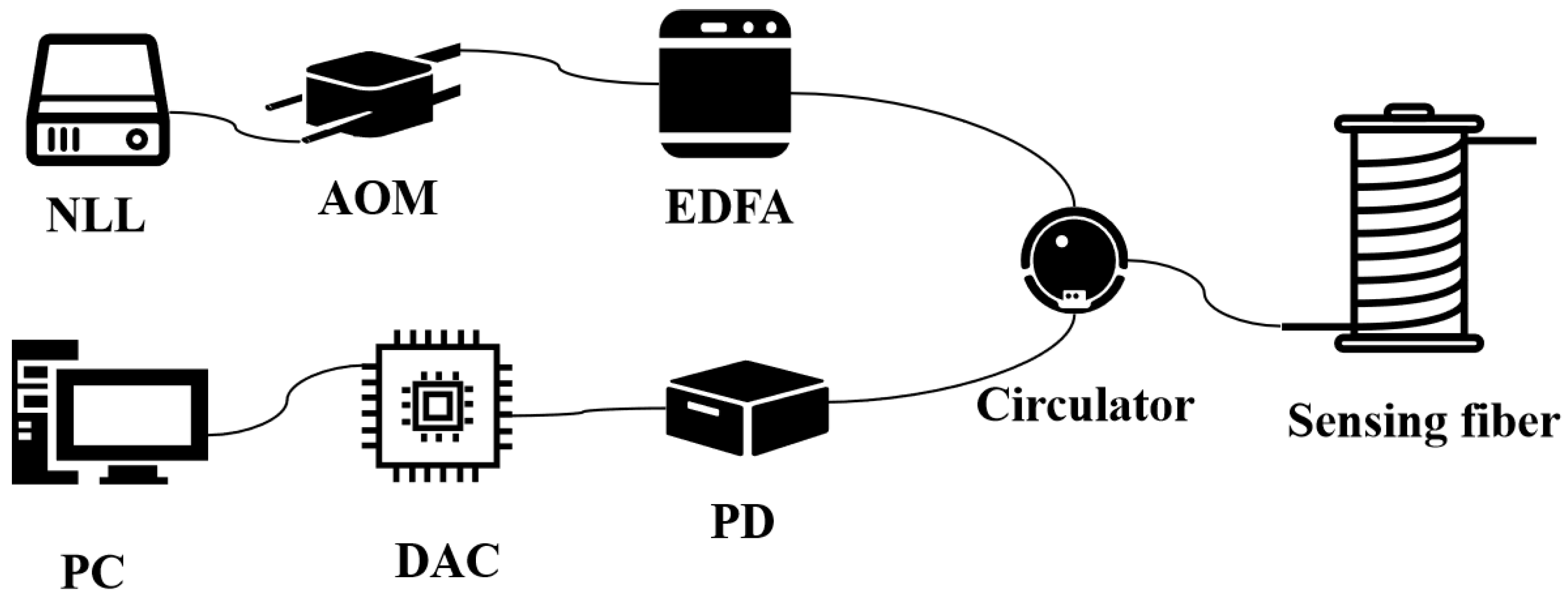
2.2. DAS System Construction
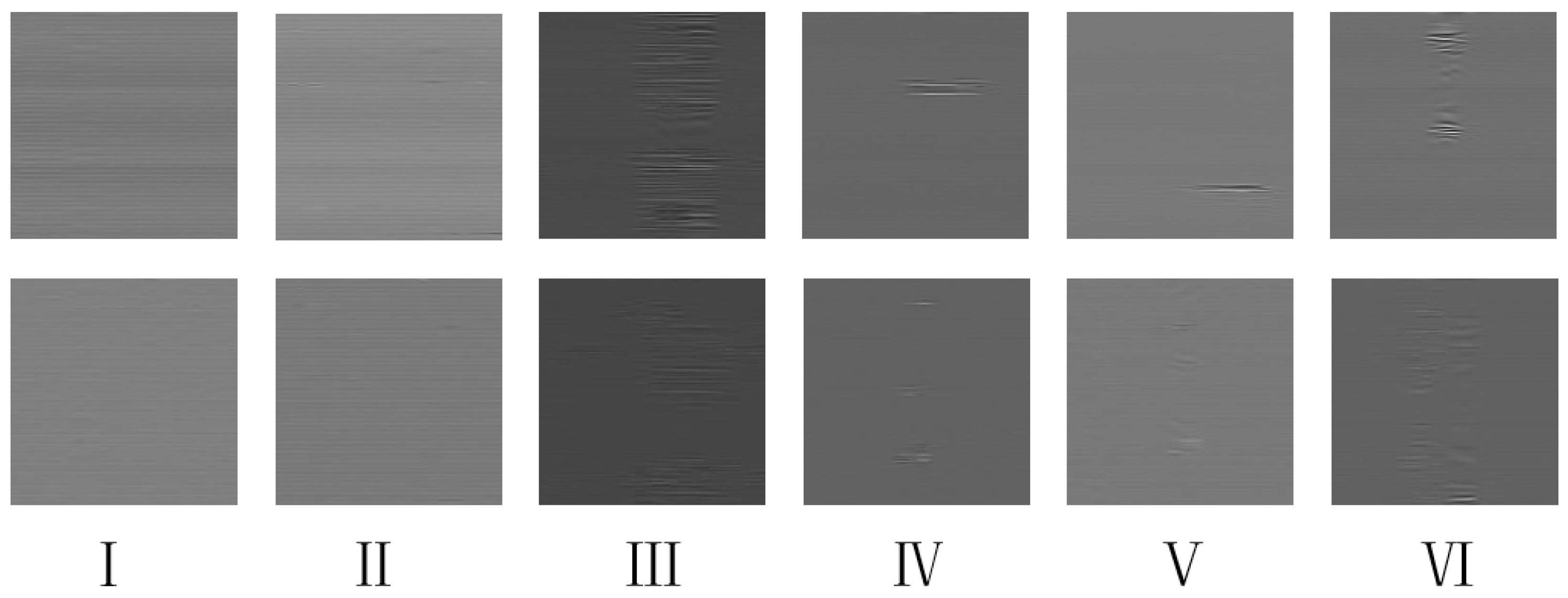
2.3. Data Preprocessing
2.4. Data Augmentation
3. Fundamental Theory of Neural Network Architecture
3.1. CNN
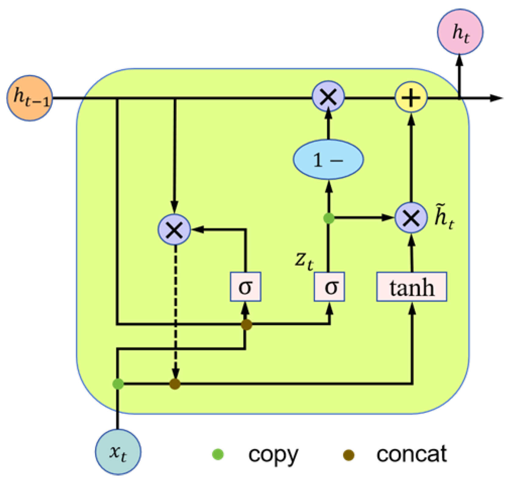
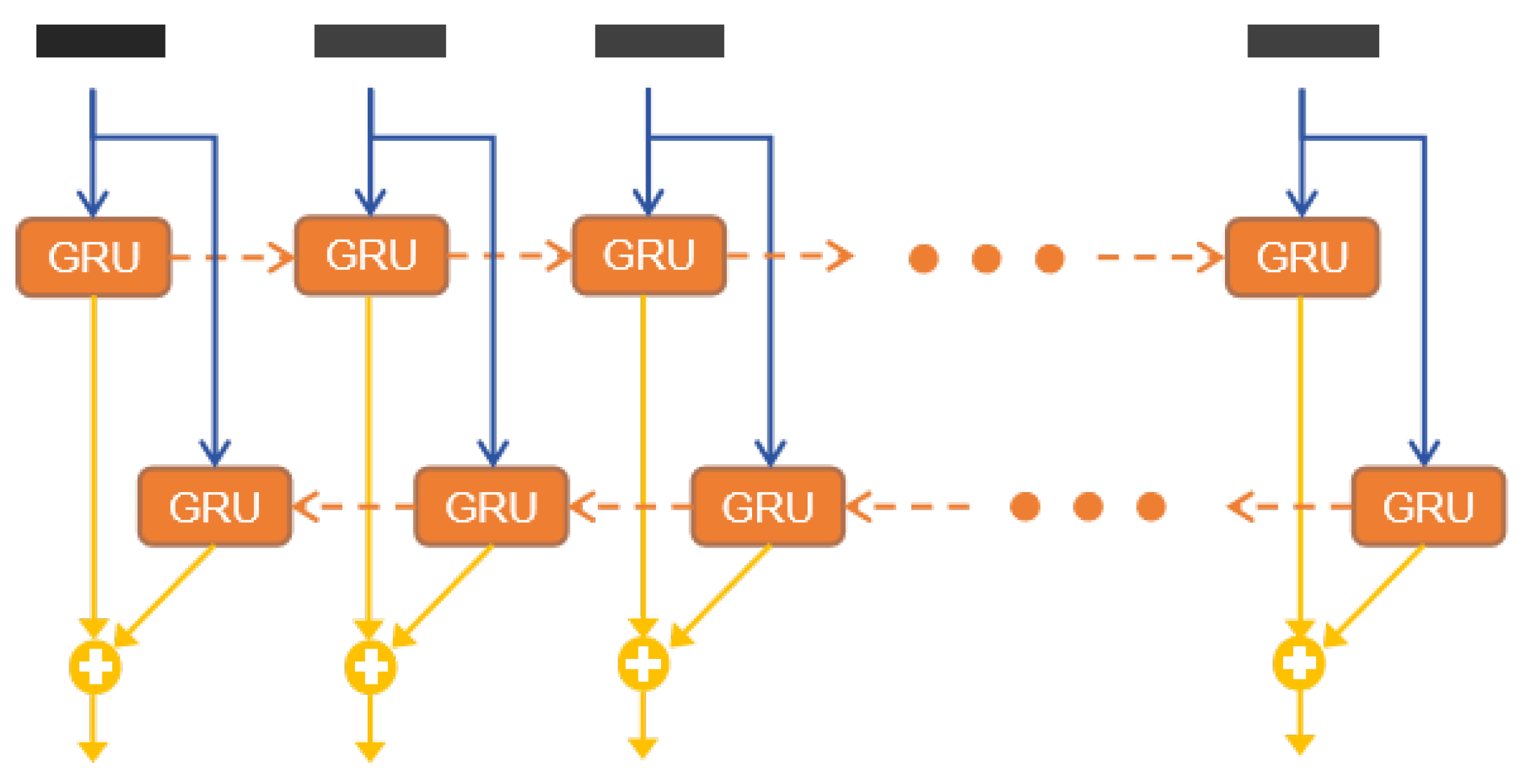
3.2. BiGRU
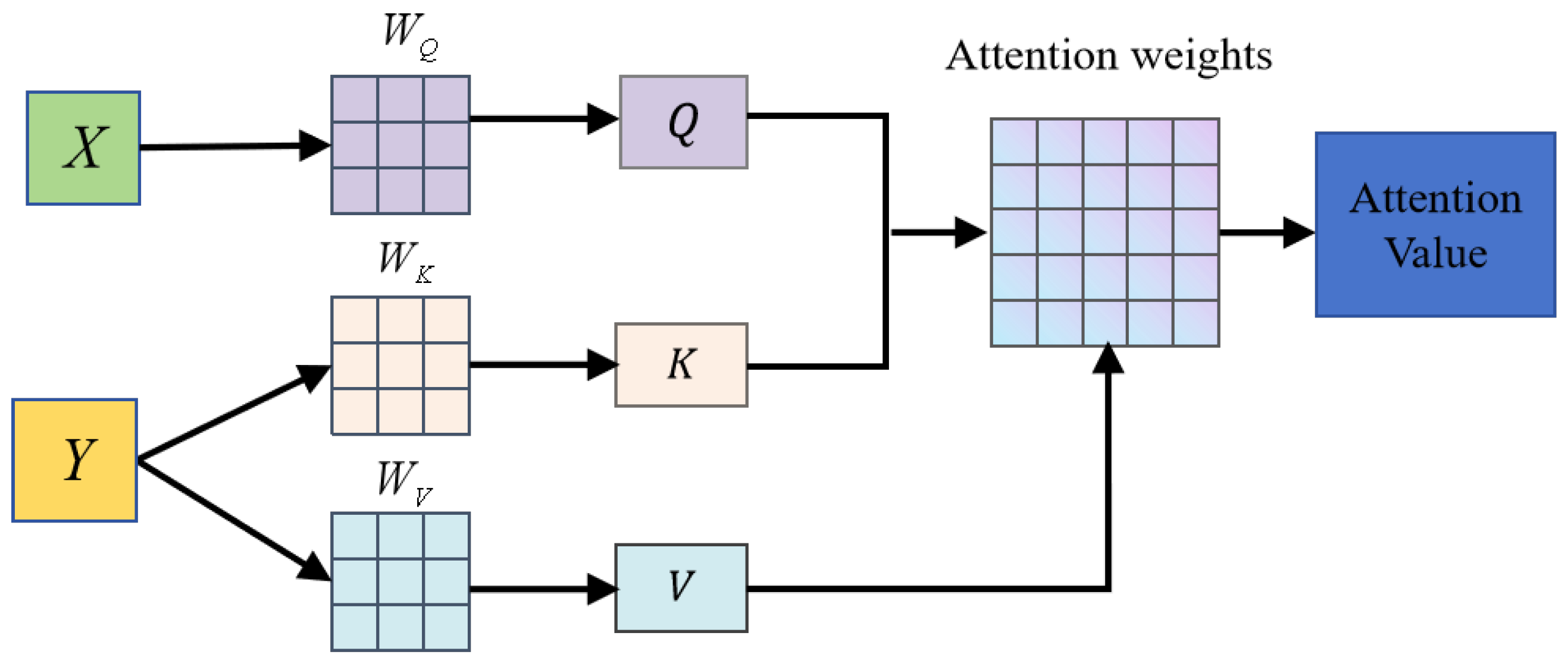
3.3. Attention Mechanism
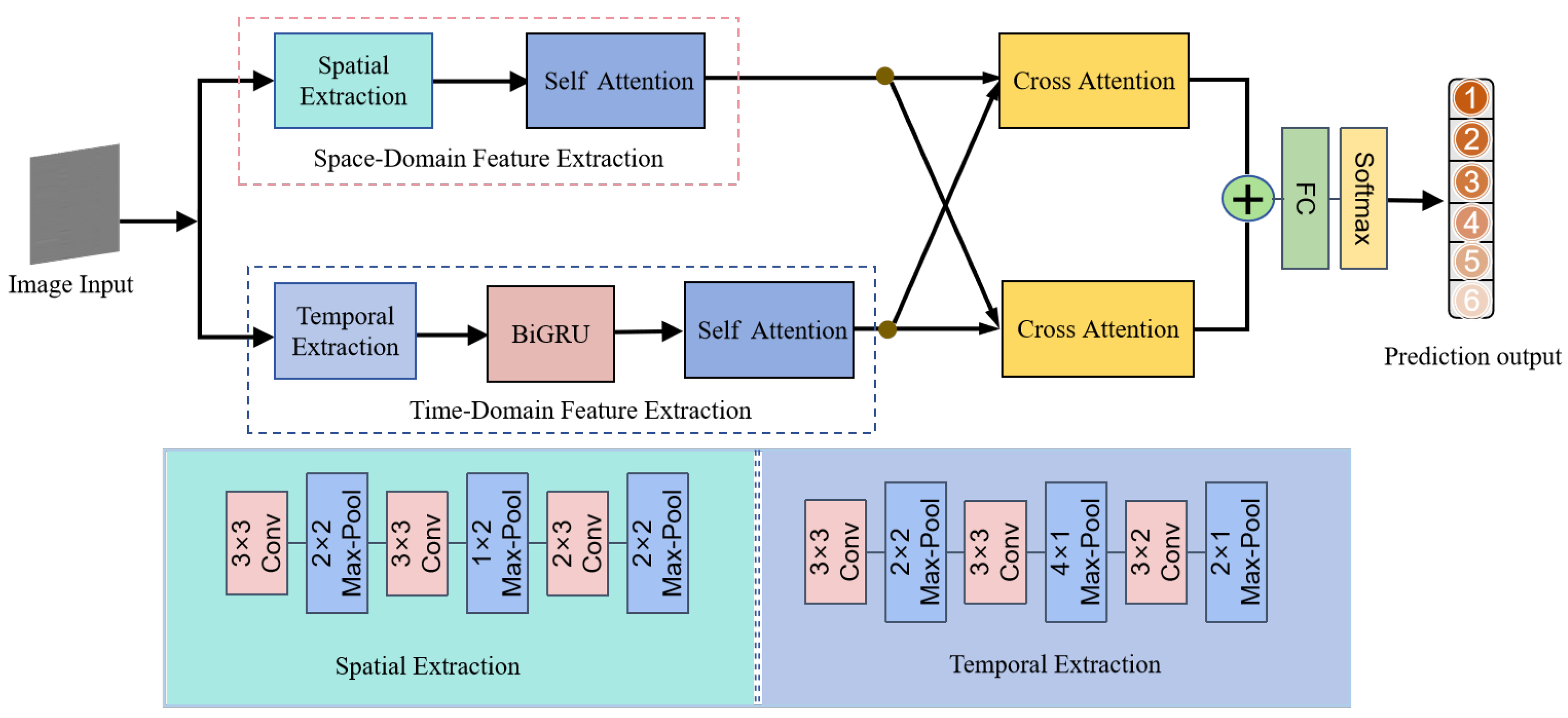
4. The Proposed CBA Model
4.1. Overall Architecture
4.2. Space-Domain Feature Extraction Module
4.3. Time-Domain Feature Extraction Module
4.4. Cross-Attention Module
4.5. FC and Softmax
5. Experimental Results and Discussion
5.1. Details for Experiments
5.2. Index
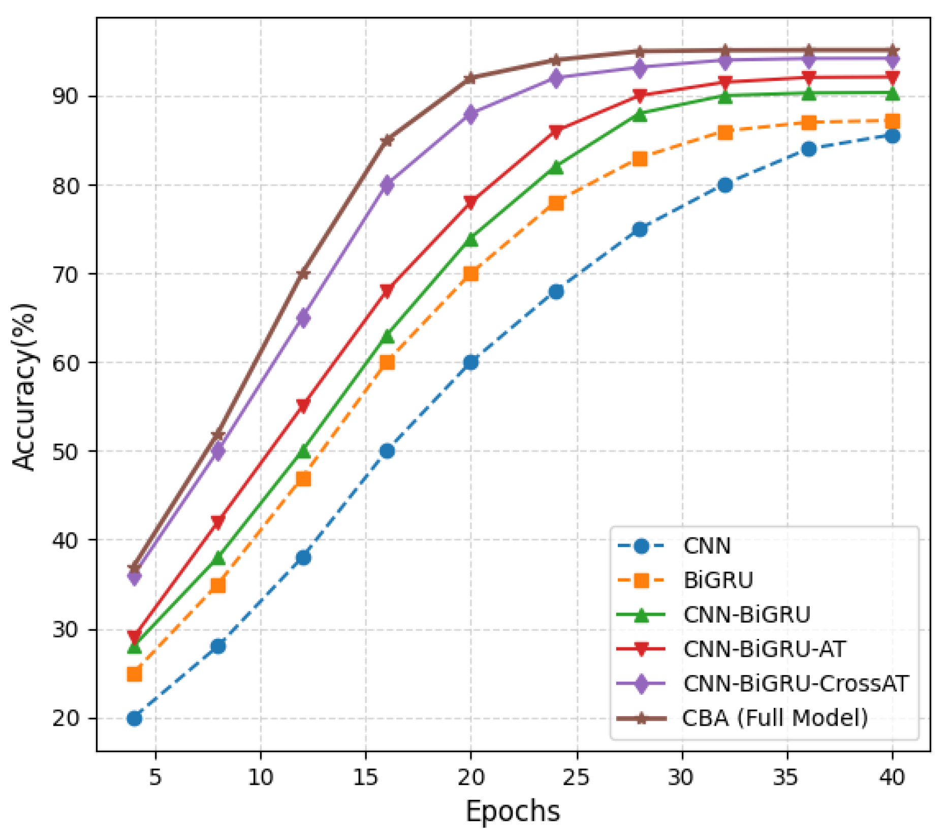
5.3. Results and Discussion
6. Conclusions
Author Contributions
Funding
Institutional Review Board Statement
Informed Consent Statement
Data Availability Statement
Conflicts of Interest
References
- Abufana, S.; Dalveren, Y.; Aghnaiya, A.; Kara, A. Variational mode decomposition-based threat classification for fiber optic distributed acoustic sensing. IEEE Access 2020, 8, 100152–100158. [Google Scholar]
- Shen, X.; Wu, H.; Zhu, K.; Liu, H.; Li, Y.; Zheng, H.; Li, J.; Shao, L.; Shum, P.P.; Lu, C. Fast and storage-optimized compressed domain vibration detection and classification for distributed acoustic sensing. J. Light. Technol. 2024, 42, 493–499. [Google Scholar]
- Zhang, X.; Ding, Z.; Hong, R.; Chen, X.; Liang, L.; Zhang, C.; Wang, F.; Zou, N.; Zhang, Y. Phase-sensitive optical time-domain reflective distributed optical fiber sensing technology. Acta Opt. Sin. 2021, 41, 0106004. [Google Scholar]
- Rao, Y.; Wang, Z.; Wu, H.; Ran, Z.; Han, B. Recent advances in phase-sensitive optical time domain reflectometry (Φ-OTDR). Photonic Sens. 2021, 11, 1–30. [Google Scholar] [CrossRef]
- Verma, S.; Mathew, J.; Gupta, S. Feature extraction based acoustic signal detection in a cost effective Φ-OTDR system. In Proceedings of the 2023 International Conference on Microwave, Optical, and Communication Engineering (ICMOCE), Bhubaneswar, India, 26–28 May 2023. [Google Scholar]
- Sun, Z.; Guo, Z. Intelligent intrusion detection for optical fiber perimeter security system based on an improved high efficiency feature extraction technique. Meas. Sci. Technol. 2024, 35, 045107. [Google Scholar]
- He, T.; Sun, Q.; Zhang, S.; Li, H.; Yan, B.; Fan, C.; Yan, Z.; Liu, D. A dual-stage-recognition network for distributed optical fiber sensing perimeter security system. J. Light. Technol. 2023, 41, 4331–4340. [Google Scholar] [CrossRef]
- Xiao, C.; Long, J.; Jiang, L.; Yan, G.; Rao, Y. Review of sensitivity-enhanced optical fiber and cable used in distributed acoustic fiber sensing. In Proceedings of the 2022 Asia Communications and Photonics Conference (ACP), Shenzhen, China, 5–8 November 2022. [Google Scholar]
- Liu, S.; Yu, F.; Hong, R.; Xu, W.; Shao, L.; Wang, F. Advances in phase-sensitive optical time-domain reflectometry. Opto-Electron. Adv. 2022, 5, 1–28. [Google Scholar]
- Yan, Y.; Khan, F.N.; Zhou, B.; Lau, A.P.T.; Lu, C.; Guo, C. Forward transmission-based ultra-long distributed vibration sensing with wide frequency response. J. Light. Technol. 2021, 39, 2241–2249. [Google Scholar]
- Yan, Y.; Zheng, H.; Zhao, Z.; Guo, C.; Wu, X.; Hu, J.; Lau, A.P.; Lu, C. Distributed optical fiber sensing assisted by optical communication techniques. J. Light. Technol. 2021, 39, 3654–3670. [Google Scholar]
- Lyu, C.; Huo, Z.; Cheng, X.; Jiang, J.; Liu, H. Distributed optical fiber sensing intrusion pattern recognition based on GAF and CNN. J. Light. Technol. 2020, 38, 4174–4182. [Google Scholar]
- Chen, J.; Li, H.; Shi, Z.; Xiao, X.; Fan, C.; Yan, Z.; Sun, Q. Low-altitude unmanned aerial vehicle detection and localization based on distributed acoustic sensing. In Proceedings of the 2023 Conference on Lasers and Electro-Optics (CLEO), San Jose, CA, USA, 7–12 May 2023. [Google Scholar]
- Wu, H.; Chen, J.; Liu, X.; Xiao, Y.; Wang, M.; Zheng, Y.; Rao, Y. One-dimensional CNN-based intelligent recognition of vibrations in pipeline monitoring with DAS. J. Light. Technol. 2019, 37, 4359–4366. [Google Scholar] [CrossRef]
- Pen, Z.; Jian, J.; Wen, H.; Gribok, A.; Chen, K.P. Distributed fiber sensor and machine learning data analytics for pipeline protection against extrinsic intrusions and intrinsic corrosions. Opt. Express 2020, 28, 27277–27292. [Google Scholar]
- Lior, I.; Rivet, D.; Ampuero, J.P.; Sladen, A.; Barrientos, S.; Sánchez-Olavarría, R.; Villarroel Opazo, G.A.; Bustamante Prado, J.A. Magnitude estimation and ground motion prediction to harness fiber optic distributed acoustic sensing for earthquake early warning. Sci. Rep. 2023, 13, 424. [Google Scholar] [CrossRef]
- Hernández, P.; Ramírez, J.; Soto, M. Deep-learning-based earthquake detection for fiber-optic distributed acoustic sensing. J. Light. Technol. 2022, 40, 2639–2650. [Google Scholar] [CrossRef]
- Ma, P.; Liu, K.; Jiang, J.; Li, Z.; Liu, T. Probabilistic event discrimination algorithm for fiber optic perimeter security systems. J. Light. Technol. 2018, 36, 2069–2075. [Google Scholar] [CrossRef]
- Wada, M.; Maeda, Y.; Shimabara, H.; Aihara, T. Manhole locating technique using distributed vibration sensing and machine learning. In Proceedings of the 2021 Optical Fiber Communications Conference and Exhibition (OFC), San Francisco, CA, USA, 6–11 June 2021. [Google Scholar]
- Pranay, Y.S.; Tabjula, J.; Kanakambaran, S. Classification studies on vibrational patterns of distributed fiber sensors using machine learning. In Proceedings of the 2022 IEEE Bombay Section Signature Conference (IBSSC), Mumbai, India, 8–10 December 2022. [Google Scholar]
- Wu, H.; Yang, M.; Yang, S.; Lu, H.; Wang, C.; Rao, Y. A Novel DAS Signal Recognition Method Based on Spatiotemporal Information Extraction With 1DCNNs-BiLSTM Network. IEEE Access 2020, 8, 119448–119457. [Google Scholar] [CrossRef]
- Chen, X.; Xu, C. Disturbance Pattern Recognition Based on an ALSTM in a Long-distance Φ-OTDR Sensing System. Microw. Opt. Technol. Lett. 2020, 62, 168–175. [Google Scholar] [CrossRef]
- Li, S.; Peng, R.; Liu, Z. A Surveillance System for Urban Buried Pipeline Subject to Third-Party Threats Based on Fiber Optic Sensing and Convolutional Neural Network. Struct. Health Monit. 2021, 20, 1704–1715. [Google Scholar] [CrossRef]
- Sun, Q.; Li, Q.; Chen, L.; Quan, J.; Li, L. Pattern Recognition Based on Pulse Scanning Imaging and Convolutional Neural Network for Vibrational Events in Φ-OTDR. J. Light Electron Opt. 2020, 219, 165205. [Google Scholar] [CrossRef]
- Shi, Y.; Li, Y.; Zhang, Y.; Zhuang, Z.; Jiang, T. An Easy Access Method for Event Recognition of Φ-OTDR Sensing System Based on Transfer Learning. J. Light. Technol. 2021, 39, 4548–4555. [Google Scholar]
- Shi, Y.; Dai, S.; Jiang, T.; Fan, Z. A Recognition Method for Multi-Radial-Distance Event of Φ-OTDR System Based on CNN. IEEE Access 2021, 9, 143473–143480. [Google Scholar] [CrossRef]
- Li, Z.; Wang, M.; Zhong, Y.; Zhang, J.; Peng, F. Fiber Distributed Acoustic Sensing Using Convolutional Long Short-Term Memory Network: A Field Test on High-Speed Railway Intrusion Detection. Opt. Express 2020, 28, 2925–2938. [Google Scholar] [PubMed]
- Li, Y.; Zeng, X.; Shi, Y. A Spatial and Temporal Signal Fusion Based Intelligent Event Recognition Method for Buried Fiber Distributed Sensing System. Opt. Laser Technol. 2023, 166, 109658. [Google Scholar] [CrossRef]
- Wu, H.; Liu, X.; Wang, X.; Wu, Y.; Liu, Y.; Wang, Y. Multi-Dimensional Information Extraction and Utilization in Smart Fiber-Optic Distributed Acoustic Sensor (sDAS). J. Light. Technol. 2024, 42, 6967–6980. [Google Scholar]
- Zhao, X.; Shan, G.; Kuang, Y.; Zhu, M. Development and Test of Smart Fiber Optic Vibration Sensors for Railway Track Monitoring. Opt. Express 2022, 30, 31123–31134. [Google Scholar]
- Hu, S.; Hu, X.; Li, J.; He, Y.; Qin, H.; Li, S.; Liu, M.; Liu, C.; Zhao, C.; Chen, W. Enhancing Vibration Detection in Φ-OTDR Through Image Coding and Deep Learning-Driven Feature Recognition. IEEE Sens. J. 2024, 24, 38344–38351. [Google Scholar]
- Wu, G.; Wang, L.; Hu, X.; Luo, Q.; Guo, D. BiGRU-DA: Based on Improved BiGRU Multi-Target Data Association Method. In Proceedings of the 2023 8th International Conference on Computer and Communication Systems (ICCCS), Guangzhou, China, 21–23 April 2023; pp. 1125–1130. [Google Scholar]
- Binlu, Y.; Guangqi, Q.; Jin, L. RUL Prediction of Rolling Bearings Based on Crested Porcupine Optimization Algorithm Optimized CNN-BiGRU-Attention Neural Network. In Proceedings of the 2024 Global Reliability and Prognostics and Health Management Conference (PHM-Beijing), Beijing, China, 21–23 April 2024; pp. 1–6. [Google Scholar]
- Murray, C.; Chaurasia, P.; Hollywood, L.; Coyle, D. A Comparative Analysis of State-of-the-Art Time Series Forecasting Algorithms. In Proceedings of the 2022 International Conference on Computational Science and Computational Intelligence (CSCI), Las Vegas, NV, USA, 14–16 December 2022; pp. 89–95. [Google Scholar]


| Hyperparameter | Value |
|---|---|
| Optimizer | Adam |
| Learning rate | 0.001 |
| Loss function | Cross-entropy loss |
| Dropout rate | 0.5 |
| GRU units | 128 (bi-directional) |
| FC layer size | 512 |
| Batch size | 32 |
| Epochs-stopping | 32 |
| Input image size | 64 × 64 × 1 |
| Number of classes | 6 |
| Method | Precision | Recall | F1-Score | NAR | Training Time (min) | Epochs | Param Count (M) |
|---|---|---|---|---|---|---|---|
| CNN | 85.52 | 85.60 | 85.56 | 14.2 | 12 | 48 | 0.45 |
| TCN | 88.47 | 88.10 | 88.28 | 10.9 | 15 | 45 | 0.60 |
| LSTM-ATTENTION | 90.90 | 90.46 | 90.46 | 9.7 | 20 | 39 | 1.40 |
| CNN-BiLSTM | 92.20 | 92.10 | 92.15 | 8.5 | 24 | 36 | 1.80 |
| CBA model | 95.13 | 95.00 | 95.06 | 6.1 | 27 | 32 | 2.10 |
| Event Type | Precision | Recall | F1-Score | NAR |
|---|---|---|---|---|
| Sunny noise | 91.10 | 91.08 | 91.09 | 12.3 |
| Rainy noise | 93.89 | 93.19 | 93.54 | 7.8 |
| Walk | 96.51 | 97.52 | 97.01 | 6.1 |
| Jump | 94.92 | 94.91 | 94.91 | 5.2 |
| Spade-shovel | 96.40 | 96.00 | 96.2 | 6.9 |
| Spade-pat | 97.00 | 97.10 | 97.05 | 3.1 |
| Model | Precision | Recall | F1-Score | NAR | p-Value vs. CBA |
|---|---|---|---|---|---|
| CNN | 85.60 | 84.90 | 85.20 | 14.2 | 7.7 × 10⁻¹⁶ |
| BiGRU | 87.20 | 86.50 | 86.90 | 12.7 | 1.9 × 10⁻¹⁵ |
| CNN-BiGRU | 90.35 | 89.90 | 90.12 | 9.6 | 1.9 × 10⁻¹³ |
| CNN-BiGRU-AT | 92.10 | 91.80 | 91.95 | 8.1 | 6.9 × 10⁻¹² |
| CNN-BiGRU-CrossAT | 94.20 | 93.70 | 93.94 | 6.8 | 1.0 × 10⁻⁸ |
| CBA (Full model) | 95.13 | 95.00 | 95.06 | 6.1 | – |
| Experiment | Precision | Recall | F1-Score | NAR |
|---|---|---|---|---|
| Exp 1 | 95.23 | 94.95 | 94.98 | 6.0 |
| Exp 2 | 94.95 | 93.81 | 95.15 | 6.3 |
| Exp 3 | 94.67 | 94.20 | 94.21 | 6.4 |
| Exp 4 | 94.68 | 94.74 | 94.58 | 6.6 |
| Exp 5 | 95.00 | 94.63 | 95.02 | 6.2 |
| Average | 94.91 | 94.47 | 94.79 | 6.3 |
Disclaimer/Publisher’s Note: The statements, opinions and data contained in all publications are solely those of the individual author(s) and contributor(s) and not of MDPI and/or the editor(s). MDPI and/or the editor(s) disclaim responsibility for any injury to people or property resulting from any ideas, methods, instructions or products referred to in the content. |
© 2025 by the authors. Licensee MDPI, Basel, Switzerland. This article is an open access article distributed under the terms and conditions of the Creative Commons Attribution (CC BY) license (https://creativecommons.org/licenses/by/4.0/).
Share and Cite
Li, C.; Chen, X.; Shi, Y. An Event Recognition Method for a Φ-OTDR System Based on CNN-BiGRU Network Model with Attention. Photonics 2025, 12, 313. https://doi.org/10.3390/photonics12040313
Li C, Chen X, Shi Y. An Event Recognition Method for a Φ-OTDR System Based on CNN-BiGRU Network Model with Attention. Photonics. 2025; 12(4):313. https://doi.org/10.3390/photonics12040313
Chicago/Turabian StyleLi, Changli, Xiaoyu Chen, and Yi Shi. 2025. "An Event Recognition Method for a Φ-OTDR System Based on CNN-BiGRU Network Model with Attention" Photonics 12, no. 4: 313. https://doi.org/10.3390/photonics12040313
APA StyleLi, C., Chen, X., & Shi, Y. (2025). An Event Recognition Method for a Φ-OTDR System Based on CNN-BiGRU Network Model with Attention. Photonics, 12(4), 313. https://doi.org/10.3390/photonics12040313