Article

A Sensitive Frequency Band Study for Distributed Acoustical Sensing Monitoring Based on the Coupled Simulation of Gas–Liquid Two-Phase Flow and Acoustic Processes

1
CNOOC Res Inst Co., Ltd., Beijing 100028, China
2
College of Petroleum Engineering, China University of Petroleum (Beijing), Beijing 102249, China
*
Author to whom correspondence should be addressed.
Photonics 2024, 11(11), 1049; https://doi.org/10.3390/photonics11111049
Submission received: 11 September 2024 / Revised: 3 November 2024 / Accepted: 5 November 2024 / Published: 7 November 2024
(This article belongs to the Special Issue Distributed Optical Fiber Sensing Technology)

Abstract

:
The sensitivity of gas and water phases to DAS acoustic frequency bands can be used to interpret the production profile of horizontal wells. DAS typically collects acoustic signals in the kilohertz range, presenting a key challenge in identifying the sensitive frequency bands of the gas and water phases in the production well for accurate interpretation. In this study, a gas–water two-phase flow–acoustic coupling model for a horizontal well is developed by integrating a gas–water separation flow model with a pipeline acoustic model. The model simulates the sound pressure level (SPL) and amplitude variations of acoustic waves under different flow patterns, spatial locations, and gas–water ratio schemes. The results demonstrate that within the same flow pattern, an increase in the gas–water ratio significantly elevates acoustic amplitude and SPL peaks within the 5–50 Hz frequency band. Analysis of oil field DAS data reveals that the amplitude response range for stages with a lower gas–water ratio falls within 5–10 Hz, whereas stages with a higher gas–water ratio exhibit an amplitude response range of 10–50 Hz.

1. Introduction

Shale gas production wells usually produce gas with water simultaneously due to the presence of groundwater and the injected water during the drilling and stimulation processes [1,2]. The accurate profiling of gas–water production is beneficial for the identification of water production and the selection of subsequent production enhancement techniques [3]. However, the interpretation of production profiles for the gas–water two-phase flow in horizontal fractured shale gas wells continues to present a significant challenge. The effectiveness of conventional electronic, acoustic, and temperature logging techniques is significantly compromised by signal interference in the long horizontal wellbore. Furthermore, the harsh downhole environment presents additional obstacles to the installation and measurement accuracy of logging instruments [4,5,6].
The rapid development of distributed fiber optic sensing technology, together with the advantages of the high precision, stability, lightweight, and compact size of optical fibers, has led to its widespread application in real-time monitoring throughout the entire lifecycle of oil and gas fields. Application areas include cementing quality evaluation, fracture morphology assessment, production profile interpretation, pipeline leak detection, and so forth [7,8,9,10].
Distributed fiber optic sensing (DFOS) can be categorized into Distributed Strain Sensing (DSS), Distributed Acoustic Sensing (DAS), and Distributed Temperature Sensing (DTS), which are based on Brillouin, Rayleigh, and Raman scattering within the fiber. When the surrounding physical fields, such as temperature, strain, and pressure, undergo change, these variations exert an effect on the laser signals transmitted within the fiber. This variation results in corresponding changes in the intensity, polarization, phase, and spectrum of the scattered light within the fiber, enabling real-time mapping and measurement of external physical field parameters [11,12].
As illustrated in Figure 1, DAS is employed to monitor fluid flow within the wellbore. During well production, reservoir fluid initially migrates from the reservoir into the fractures. Subsequently, these fluids traverse fractures that have been filled with proppant material, flow through perforation tunnels, and eventually enter the wellbore. In the near-wellbore region, fluid experiences high velocities within the fractures and perforation clusters, which induce turbulent flow. This turbulent flow generates acoustic pressure waves that are transmitted to the optical fiber. The fiber may be installed outside the casing, outside the tubing, inside the tubing, or deployed along with coiled tubing. When these pressure vibration-induced acoustic waves act on the optical fiber along the wellbore, the fiber undergoes axial displacement due to compression. This results in phase shifts of Rayleigh backscattered light within the fiber [13]. The phase is related to the change in fiber length as follows [14]:
Δ Φ = Φ Δ L L + Δ n n
where Φ is the optic phase; Δ L is the fiber axial displacement; Δ L L is the fiber axial strain; Δ n n is the relative change fiber refractive index.
The sound pressure level is the ratio of the sound pressure to a reference acoustic pressure:
L p = 20 log 10 p p 0
where L p is the sound pressure level, dB; p is the actual measured sound pressure, Pa; and p 0 is the reference sound pressure, Pa.
The sound amplitude represents the amplitude of the sound pressure, both of which are parameters used to describe sound pressure. By demodulating the DAS phase, the acoustic pressure information during fluid flow can be obtained, allowing for the calculation of sound pressure level and sound wave amplitude. Performing a Fourier transform on the DAS signal allows for the analysis of sound pressure level and sound wave amplitude responses across different frequency bands.
The use of DAS acoustic signals for monitoring multiphase flow in horizontal wells has experienced a broadening of its application scope. During fracturing injection, Jayaram [15] and Pakhotina [16] in their study calculated the DAS acoustic energy of each perforation cluster to determine the volumetric distribution of injected fluids and proppants within the clusters. Li [17] calculated the fluid and proppant volumes for each cluster by computing the relative acoustic intensity at each point along the measured depth of a horizontal well over time. Other researchers, such as Peter [18] and Bukhamsin [19], have employed the fluid phase fraction/rate determined by the acoustic velocity of DAS in fluids as input parameters for completion design models, optimizing completion designs, or conducting reservoir history matching to enhance the predictive capability of reservoir models. During the production phase, Horst [20] successfully converted DAS acoustic energy within a specific frequency range into flow rates, providing a quantitative interpretation of gas production from different production stages and periods. Moradi [21] devised a systematic workflow for processing DAS acoustic data using the Frequency–Wavenumber (F–K) analysis method to calculate acoustic flow velocity and evaluate phase volume fractions in multiphase flows, including oil–gas, water–oil, and oil–gas–water scenarios. The workflow was validated with experimental data.
Nevertheless, current research on the response mechanisms of DAS acoustic signals to the fluid composition, flow patterns, and flow development processes of multiphase fluids in the wellbore during production remains inadequate. The sensitive frequency bands for different gas–water two-phase flow patterns remain unclear. Through this study, we aim to elucidate the underlying mechanisms through which gas–water two-phase flow correlates with the varying acoustic signal response frequencies. A gas–water two-phase flow–acoustic coupling model for a horizontal well is developed by integrating a gas–water separation flow model with a pipeline acoustic model. The model simulates the sound pressure level (SPL) and amplitude variations of acoustic waves under different flow patterns, spatial locations, and gas–water ratio schemes. The sensitive frequency bands for typical gas–water flow conditions in shale gas production wells are determined. Lastly, the numerical simulation conclusions are verified using real DAS data from the production process of a field horizontal well.

2. Methods

The objective of the process described in this section is to develop a coupled flow–acoustic numerical model for simulating gas–water separation flow and the resulting acoustic field in a horizontal wellbore. The pressure field will be employed as the coupling variable to simulate DAS acoustic signals and perform calculations using finite element software. Three flow patterns were simulated, and corresponding acoustic signals related to increasing gas–water ratios within each flow pattern were analyzed. The flow patterns of gas–liquid two-phase flow in horizontal wells exert a considerable influence on fluid flow acoustic signals. Mandhane [22] classified gas–liquid flow patterns in horizontal pipes into the following categories based on the superficial velocity of gas and liquid (Figure 2): bubble flow, slug flow, stratified flow, wave flow, annular flow, and dispersed flow. The Mandhane flow pattern diagram is applicable to horizontal pipes with an inner diameter ranging from 12.7 to 165.1 mm. Considering that the typical pipeline size of horizontal shale gas wells in the field is around 120 mm, it falls within the pipeline size applicable range of the Mandhane flow pattern diagram.
We will simulate the acoustic signal characteristics generated by different flow patterns in the wellbore to explore the relationship between gas–water two-phase flow patterns and their corresponding acoustic signals.

2.1. Gas–Water Separation Flow Model in Horizontal Wellbores

The gas–water separation flow model assumes that the gas and water phases flow separately, each with its own flow velocity and physical parameters. In order to establish the flow model, it is necessary to create individual models for each phase and then couple them together [24]. We selected a horizontal well segment dz as the object of study, with a flow segment diameter D and a cross-sectional flow area A (Figure 3). The angle θ between the wellbore and the horizontal direction is typically small for horizontal wellbores.

2.1.1. Mass Balance Equation

According to the law of conservation of mass, we have
G = C .
The differential form of the mass equation is
d G g = Gdx = d ( ρ g ν g A g )
d G w = Gd 1 x = Gdx = d ρ w ν w A w ,
where G is the mass flow rate in the wellbore, kg/s; ρ is the fluid density, kg/m3; ν is the actual velocity of the fluid, m/s; A is the area occupied by the fluid in the cross-section, m2; x = Gg/G is the mass gas fraction; g represents the gas phase; w represents the water phase.

2.1.2. Momentum Balance Equation

The momentum balance equation for the gas phase is
p A g p + dp A g d F g τ ρ g g A g d τ sin θ = G g + d G g ν g + d ν g G g ν g ν w d G g ,
where dFg is the frictional resistance of the gas phase in contact with the pipe wall and τ is the shear stress at the gas–water interface.
The momentum balance equation for the water phase is
p A w ( p + dp ) A w d F w + τ ρ w g A w dzsin θ = G w + d G w ν w + d ν w G w ν w ν w d G w .
Substituting the cross-sectional gas fraction ϕ = Ag/A and liquid fraction 1 − ϕ = Aw/A and dividing each term by Adz while omitting higher-order small quantities, we obtain the differential momentum equations for the separation flow model:
dp dz = 1 A dF dz + g sin θ [ ϕ ρ g + ( 1 ϕ ) ρ g ] + G A 2 d dz x 2 v g ϕ + ( 1 x ) 2 v w 1 ϕ

2.1.3. Energy Balance Equation

For the separation model, it is necessary to consider the energy equations for both the gas and water phases. By summing the energy balance equations for each phase, the total energy balance per unit time can be expressed as follows:
x ν g + ( 1 x ) ν w dp dz = gsin θ + G A 2 d dz x 3 ν g 2 2 ϕ 2 + ( 1 x ) 3 ν w 2 2 ( 1 ϕ ) 2 + dE dz
where dE / dz represents the mechanical energy loss per unit flow segment.

2.2. Gas–Water Two-Phase Acoustic Model in Horizontal Wellbores

Lighthill [25] proposed the classic aero-acoustic model based on the Navier–Stokes equation:
2 ρ t 2 c 0 2 ρ x i 2 = 2 T ij x i x j
where T ij = ρ υ i υ j + p c 0 2 ρ δ ij σ ij is the Lighthill tensor; ρ is the fluid density, kg/m3; υ is the fluid velocity, m/s; p is the fluid sound pressure, MPa; c 0 is the sound speed, m/s; δ ij is the Kronecker delta; σ ij is the fluid viscous stress tensor.
Based on the Lighthill equation, Williams [26] further considered additional fluid noise terms and derived the Ffowcs Williams–Hawkings (FW–H) equation:
2 ( ρ H ( f ) ) t 2 c 0 2 2 ( ρ H ( f ) ) x i 2 = t ρ 0 V i f x i δ f x i ( p δ ij σ ij ) f x j δ f + 2 x i x j ( T ij H ( f ) )
where H ( f ) is the boundary control surface equation describing the moving object; thus, we have
δ ( f ) = H f f ,
and V i = x i / t represents the components of the object’s surface velocity along the x i direction.
In the context of the FW–H equation, the right-hand-side terms represent three sources of noise in two-phase flow, including monopole sources, dipole sources, and quadrupole sources. In this study, the gas–water two-phase flow model initiates the mixing process at the designated inlet. The disparate velocities of gas–water phases result in a turbulent two-phase flow and significant interactions at the pipe wall that generate pressure pulses, forming dipole noise sources. Therefore, in this study, we only consider the impact of dipole noise. In the case where only dipole sources are present, Equation (9) is transformed to
2 ρ H ( f ) t 2 c 0 2 2 ρ H ( f ) x i 2 = x i p δ ij σ ij f x j δ ( f ) .

2.3. Numerical Model

2.3.1. Model Parameters

A three-dimensional pipeline model was established, with a pipeline length of 3 m and a diameter of 0.12 m (Figure 4). To enable the independent setting of gas- and water-phase velocities in the two-phase separation model, the pipeline inlet was designed as annular, with the gas and water phases entering into different cross-sectional areas. The diameter of the gas inlet was set to 0.08 m, whereas the water inlet annular diameter was set to 0.04 m, with the inlet cross-sectional areas for both gas and water set to 0.005 m2, with this value chosen to eliminate the influence of the geometric settings on the simulation results. At the initial stage of the simulation, the entire pipeline was filled with gas, and the gas and water phases mixed at the inlet, subsequently forming a two-phase flow along the pipeline. To enhance the quality of the mesh and ensure greater computational accuracy, the pipeline wall, inlet, and outlet were also subjected to mesh refinement.
Six different cases were constructed based on the flow patterns of gas–water two-phase flow, the gas–water ratio, and the surface gas and water flow rates. Table 1 shows the parameters for each case. The surface gas and water flow rates were converted from the flow velocity within the pipeline, with the converted flow rate falling within the flow rate range of shale gas horizontal wells. The gas volume factor was 0.0035, the natural gas density was 0.7 kg/m3, and the viscosity was 1.2 × 10⁻⁵ kg/(m·s); the water density was 989 kg/m3, and the viscosity was 8.9 × 10⁻⁴ kg/(m·s).
Four points were set up in the pipeline model, with their specific locations shown in Figure 5. From point 1 to point 4, the distance from the inlet increases gradually. The characteristics of the acoustic field generated by the two-phase flow at different locations were analyzed.

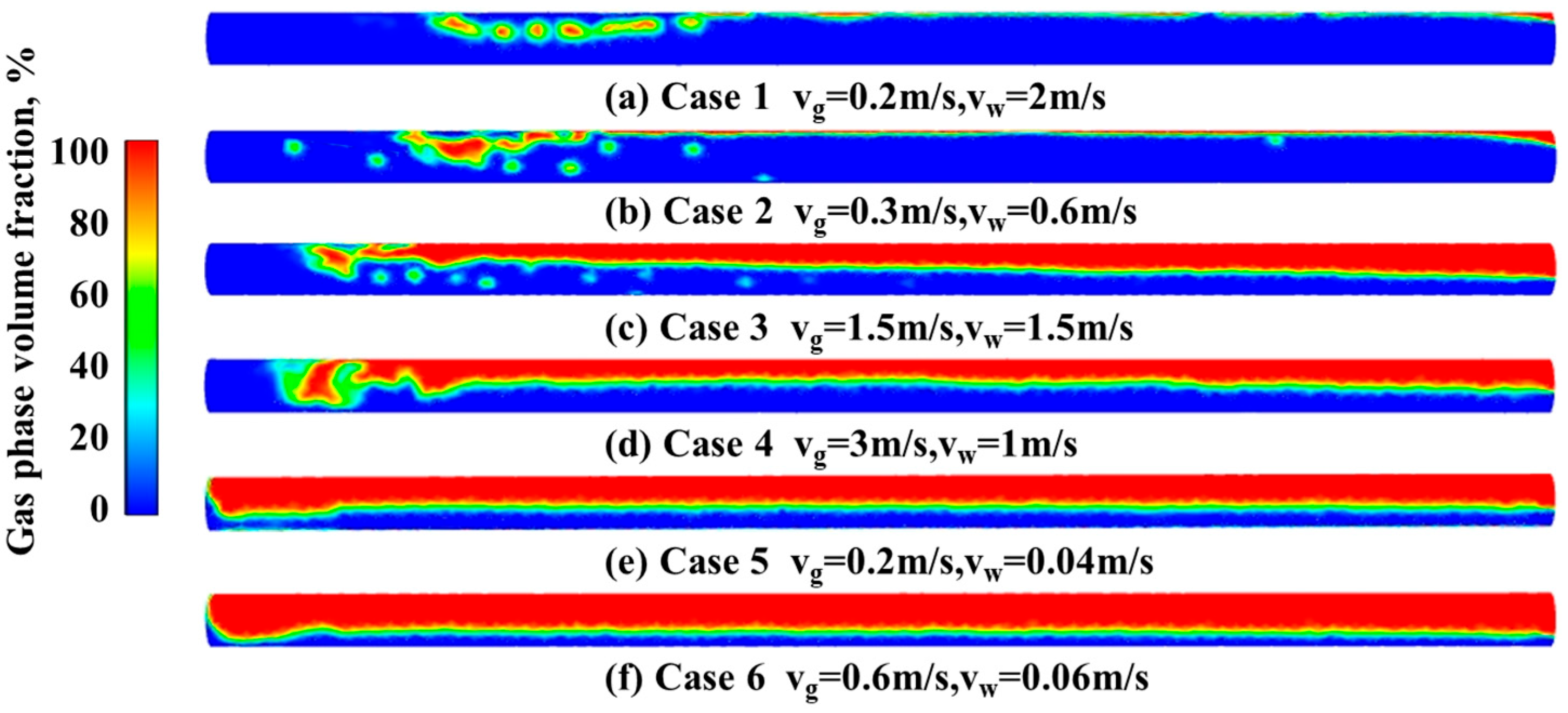
2.3.2. Basic Simulation Results

Figure 6 shows the distribution of gas–phase volume fractions after the gas–water two-phase flow fully passes through the pipeline under the conditions of each case, providing a clear visualization of the flow patterns at different velocities and gas–water ratios.
Cases 1 and 2 exhibit bubbly flow. As the gas–water ratio increases from 0.1 to 0.5, the dispersed bubbles begin to coalesce. Cases 3 and 4 exhibit slug flow. As the gas–water ratio increases from 1 to 3, the dispersed bubbles have completely disappeared, and only segmented slugs appear. Cases 5 and 6 exhibit stratified flow. As the gas–water ratio increases from 5 to 10, the stratified interface lowers, indicating an increased proportion of the gas phase. Figure 6 demonstrates that as the gas–water ratio increases, the two-phase flow pattern transitions from bubbly flow to slug flow and then to stratified flow. Figure 7 shows the corresponding flow patterns of each scenario in the Mandhane flow pattern map. It can be observed that the expected flow patterns are consistent with the actual simulation results.

3. Results

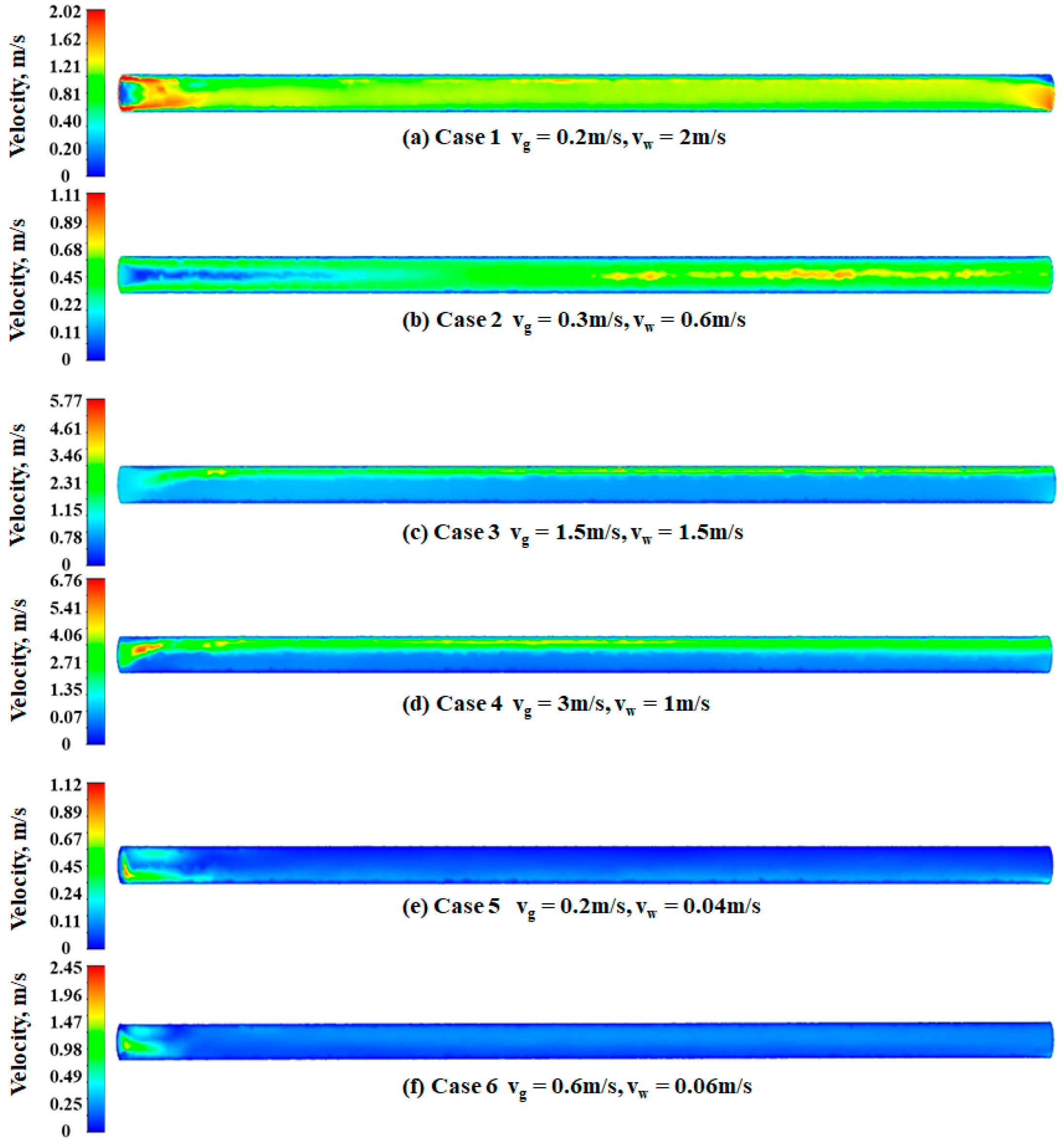
3.1. Velocity Field of Gas–Water Two-Phase Flow

Figure 8a,b show the velocity distribution plots for Cases 1 and 2, both of which exhibit bubbly flow. The gas-phase velocity is lower than the liquid-phase velocity, with a noticeable velocity mixing region at the inlet and no distinct velocity interface.
Figure 8c,d show the velocity distribution plots for Cases 3 and 4, which exhibit slug flow. The gas-phase velocity is similar to or greater than the liquid-phase velocity, with the gas phase rising after mixing with the liquid at the inlet and forming a distinct velocity interface in the downstream section of the pipeline.
Figure 8e,f show the velocity distribution plots for Cases 5 and 6, which exhibit stratified flow. The gas-phase velocity is significantly greater than the liquid-phase velocity, resulting in a velocity mixing region at the inlet, with the gas phase dominating in the downstream section. Overall, the gas- and water-phase velocities are relatively similar within the same flow pattern.

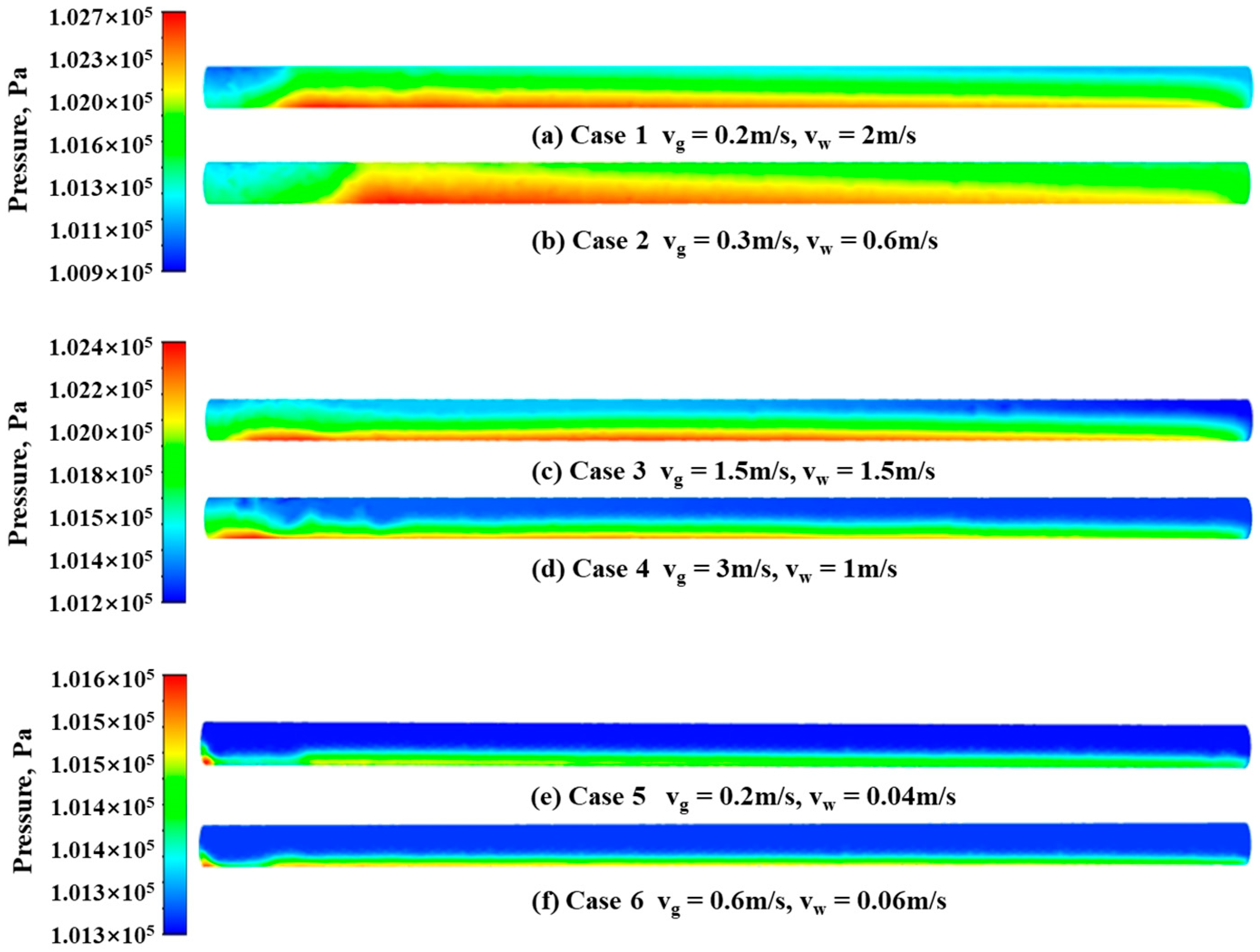
3.2. Pressure Field of Gas–Water Two-Phase Flow

The acoustic model simulates the noise source as pressure pulses generated by the interaction between the gas and water phases. Consequently, analysis of the pressure distribution characteristics for different flow patterns in the horizontal pipeline is required.
Figure 9a,b show the pressure distribution for Cases 1 and 2 (bubbly flow), where there is significant pressure variation in the middle of the pipeline, corresponding to the appearance of bubbles in the flow pattern diagram.
Figure 9c,d show the pressure distribution for Cases 3 and 4 (slug flow), where large pressure variation can be observed at the gas–water mixing point near the inlet, which aligns well with the flow pattern diagram.
Figure 9e,f show the pressure distribution for Cases 5 and 6 (stratified flow), where the pressure variation is minimal. The pressure variation is concentrated near the gas–water inlet, with minimal subsequent pressure changes. These results indicate that the turbulence between the two-phase flows is minimal, with turbulence primarily occurring at the inlet.

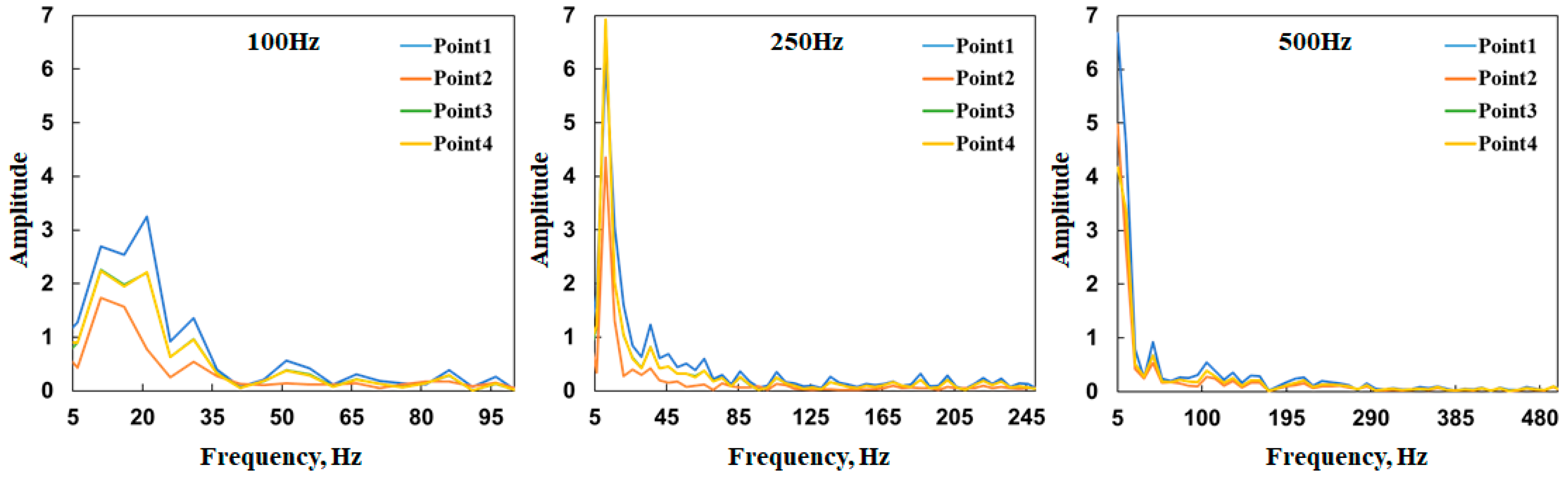
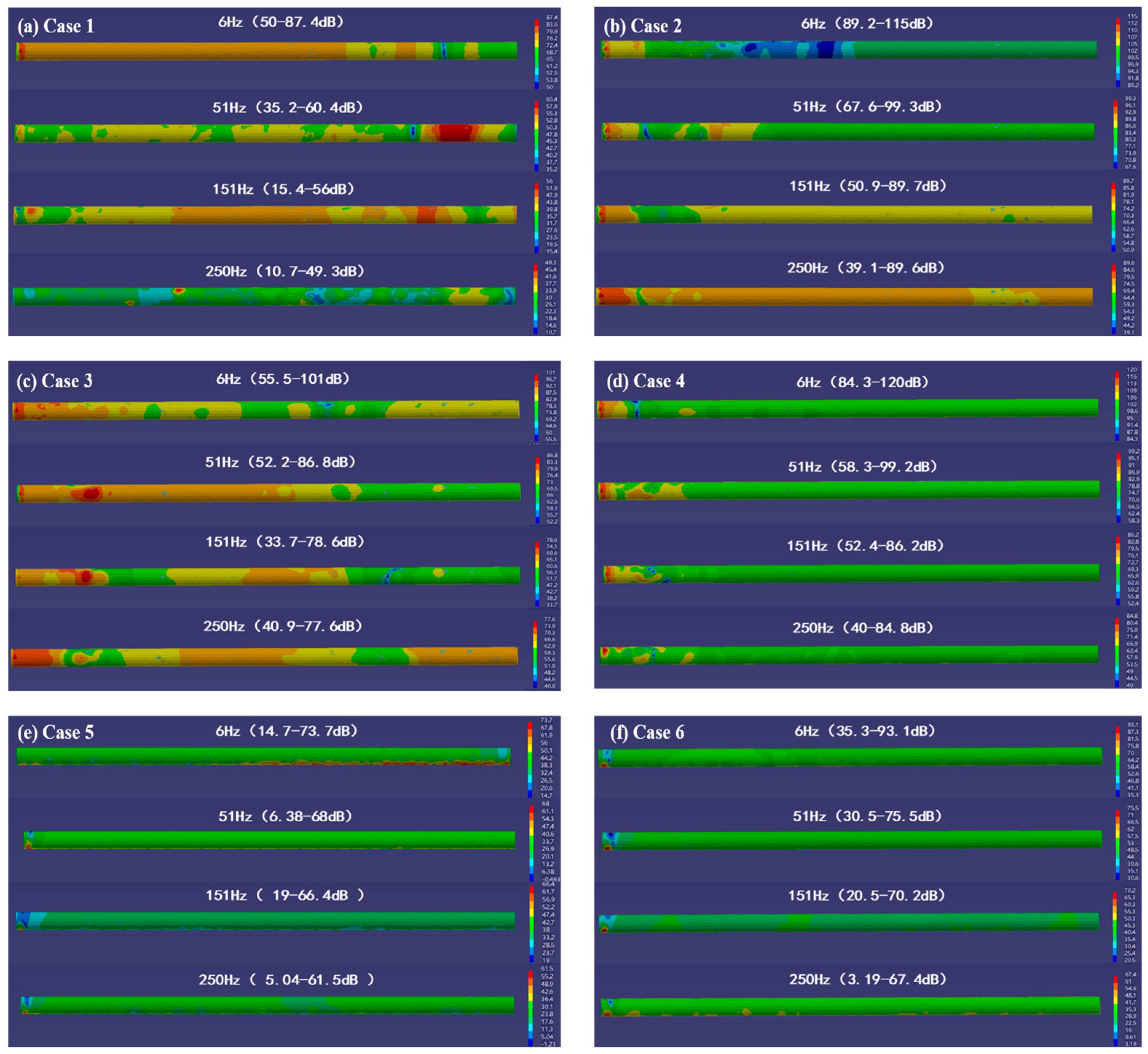
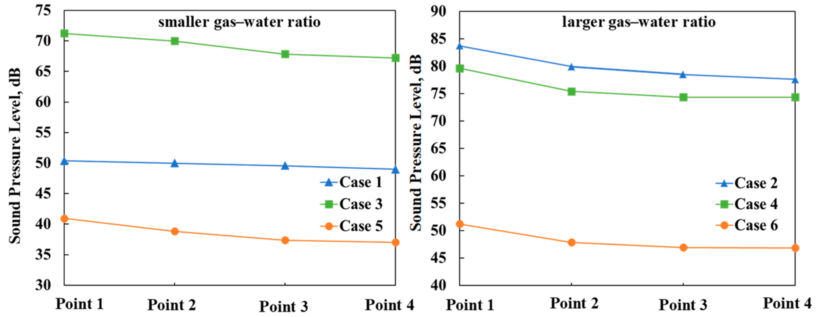
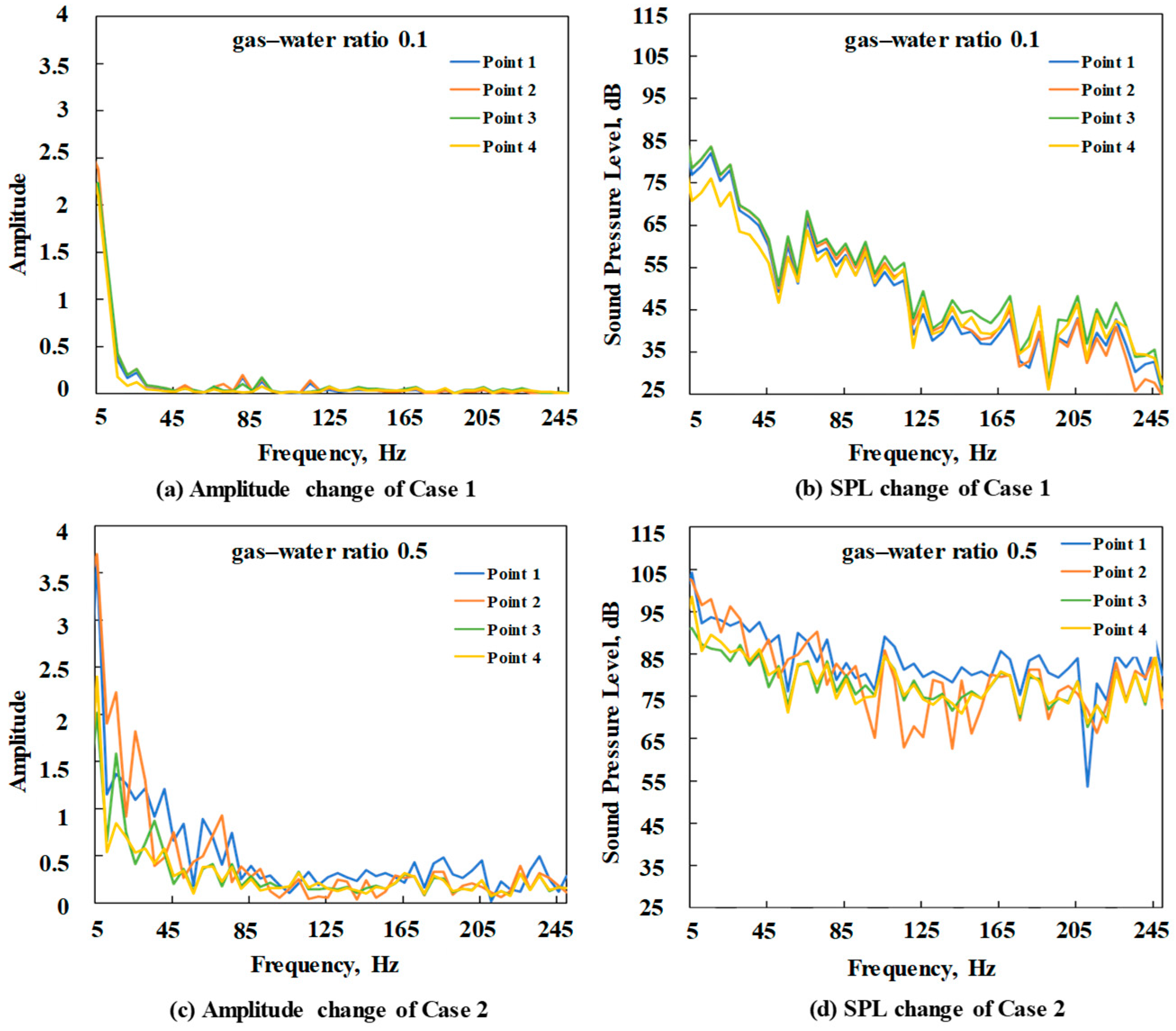
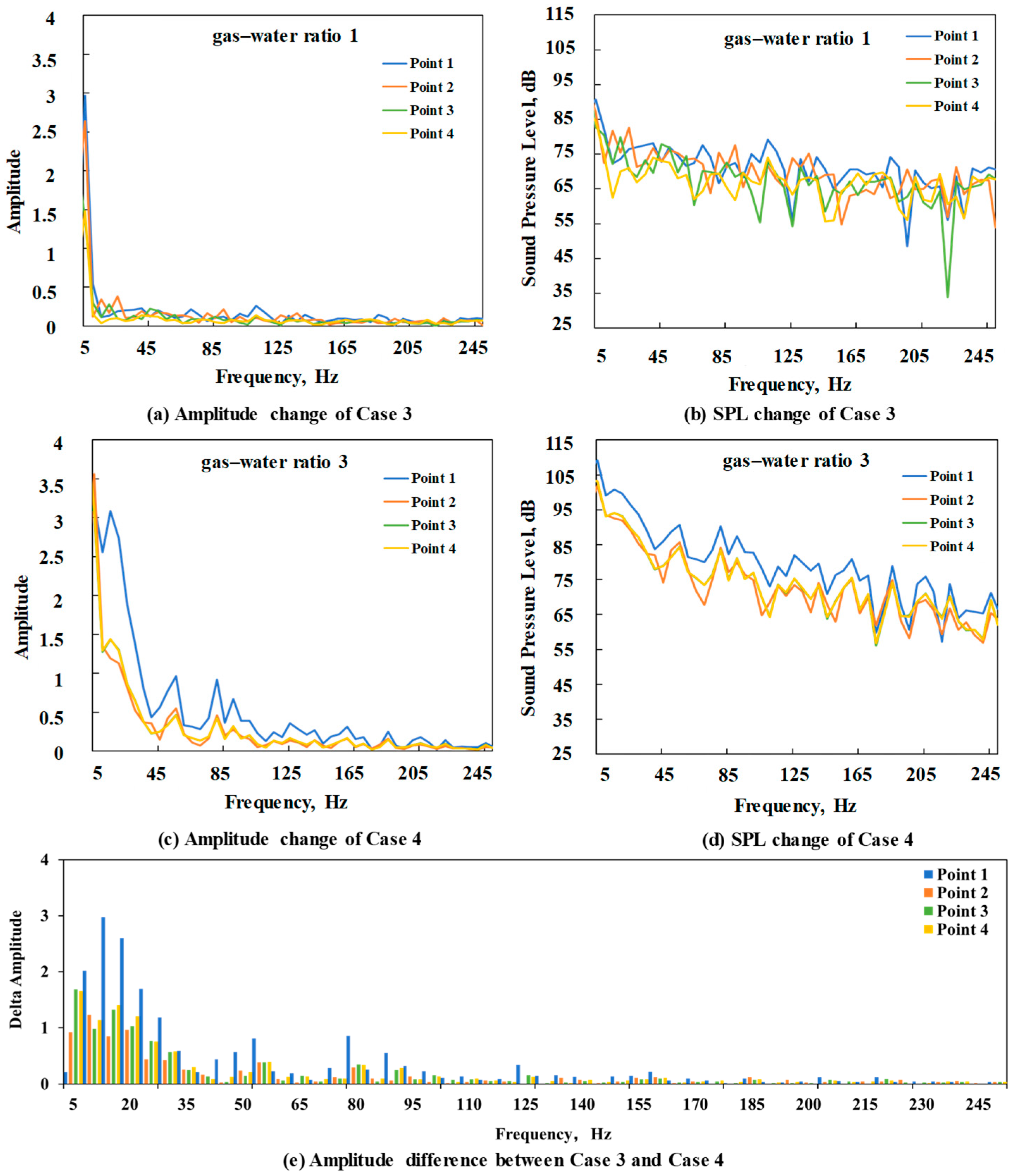
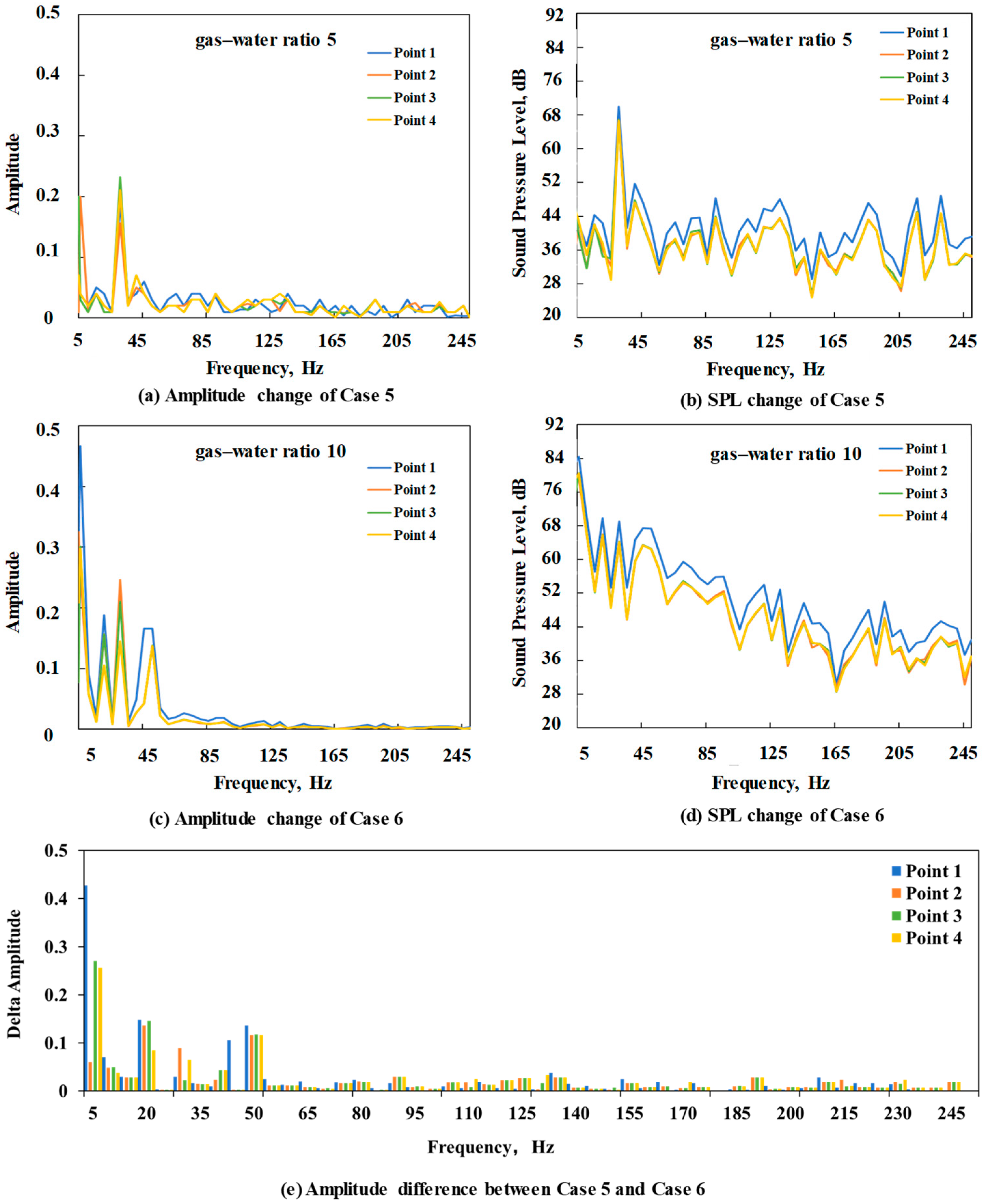
3.3. Sound Field of Gas–Water Two-Phase Flow

For production monitoring, the highest identifiable frequency of DAS data is typically 1000 Hz. Therefore, in this study, we primarily focused on acoustic signals below 1000 Hz. The simulated acoustic field in this study considers maximum frequencies of 100 Hz, 250 Hz, and 500 Hz, corresponding to the respective acoustic wave amplitudes. The amplitude curves are shown in Figure 10, where the region near 0 Hz is affected by direct current components. Therefore, all acoustic simulation results are recorded starting from 5 Hz. Figure 10 illustrates that the amplitude peaks are concentrated between 5 and 125 Hz, with no significant peaks above 250 Hz. Accordingly, the maximum frequency for acoustic simulation in this study was set to 250 Hz. The sound pressure level (SPL) distribution at four frequencies including 6 Hz, 51 Hz, 151 Hz, and 250 Hz was selected for analysis. Subsequently, the variation in SPL with increasing frequency was investigated for each case, and the findings were compared with the pressure distribution plots of the flow field to ascertain the degree of alignment.
A comparison of the SPL distribution across different frequencies under all case conditions indicates that the SPL exhibits a gradual decrease as the frequency increases. In the case of bubbly flow (Figure 11a,b) and slug flow (Figure 11c,d), the SPL demonstrates notable variation, exhibiting a rapid change near the inlet and a gradual change along the middle and rear sections of the pipeline. This trend is consistent with the pressure distribution plots of bubbly and slug flow (Figure 9), reinforcing the consistency of the observed behavior across different flow regimes. For stratified flow (Figure 11e,f), the SPL variation is confined to the gas–water mixing region near the inlet, with no appreciable changes in the middle and rear sections of the pipeline. The SPL variation trend aligns with the pressure distribution plots of stratified flow (Figure 9).
Figure 12 depicts the mean SPL trend across the field points for the six cases. As the distance between the field point and the inlet increases, the mean SPL decreases gradually. This finding suggests that the closer the field point is to the inlet, the greater the pressure pulses generated by the interaction of the gas–water two-phase flow.
At a given point, it can be observed that the SPL for bubbly flow (Case 1 and Case 2) and slug flow (Case 3 and Case 4) is greater than that for stratified flow (Case 5 and Case 6). This finding is consistent with the results reported by Wang [27]. This finding is due to the fact that the interaction between the gas and water phases in slug flow and bubbly flow is more pronounced, resulting in elevated turbulence and amplified pressure pulse fluctuations on the pipe wall. Consequently, these factors have an impact on the acoustic response.
A higher gas–water ratio within the same flow pattern results in a greater sound pressure level (SPL). This change is due to the increased volume of the gas phase, which in turn leads to higher turbulence in the two-phase flow.
Further analysis of the SPL and amplitude variations at different locations for each case was conducted to investigate the effect of the gas–water ratio on the SPL and amplitude within the same flow pattern and to explore the corresponding response frequency bands for the gas and water phases. For bubbly flow (Figure 13), slug flow (Figure 14), and stratified flow (Figure 15), an increase in the gas–water ratio was observed to consistently result in elevated levels of the SPL and amplitude response peaks.
In bubbly flow, when the gas–water ratio is 0.1, a significant acoustic amplitude response is observed in 5–10 Hz. As the gas–water ratio increases to 0.5, the amplitude rises to varying levels across 5–250 Hz. Figure 13e illustrates the difference in acoustic amplitude before and after the increase in the gas–water ratio. It can be observed that each point exhibits a greater amplitude increase within 5–80 Hz, indicating that the frequency range of the acoustic amplitude response expands with an increased gas–water ratio. Additionally, the overall SPL increases as the gas–water ratio rises, but no specific frequency range shows a significant increase in the SPL. The SPL at point 1, located near the fluid inlet, demonstrates a notable increase, consistent with the observations in Figure 12, where the SPL at point 1 is higher than at other points in cases with elevated gas–water ratios.
In slug flow, when the gas–water ratio is 1, a significant acoustic amplitude response is observed in the range of 5–10 Hz. As the gas–water ratio increases to 3, a notable increase in amplitude is observed across 5–80 Hz (Figure 14e), with more pronounced increases at Points 1 and 2, which are closer to the fluid inlet. The SPL shows an increasing trend across all frequencies, with Point 1 exhibiting the largest response. Compared to other frequency ranges, the SPL is particularly elevated in the 5–50 Hz range.
In stratified flow, when the gas–water ratio is 5, two distinct acoustic amplitude peaks are observed within 5–40 Hz. As the gas–water ratio increases to 10, a significant amplitude increase is observed within 5–50 Hz (Figure 15e), with Point 1 demonstrating a higher increase. The SPL exhibits an increasing trend across all frequencies, with Point 1 displaying the highest response. Compared to other frequency ranges, the SPL is notably higher in the 5–50 Hz range, while the SPL at other points converges, forming a single curve.
Overall, as the gas–water ratio of the three flow patterns increases, both the amplitude and SPL increase within the range of 0–250 Hz, with a more significant response peak observed in 5–50 Hz. After the increase in the gas–water ratio, the high-amplitude response frequency of bubble flow and slug flow expands from 5–10 Hz to 10–50 Hz. The stratified flow pattern, which inherently has a higher gas–water ratio, shows an expansion of high-amplitude frequency from 5–40 Hz to 5–50 Hz. Additionally, it can be observed that after the increase in the gas–water ratio, the amplitude and SPL at observation Point 1 increase more significantly within the 0–250 Hz range compared to other observation points, with the increase in SPL being more pronounced than that of the amplitude. From the above numerical simulation results, it can be concluded that the sensitive response frequency range of the water phase during gas–water two-phase flow is 5–10 Hz, while that of the gas phase is 5–50 Hz. Based on this, subsequent analyses of DAS data from production well stages will primarily focus on data within the 5–10 Hz and 5–50 Hz ranges, with data collection occurring near the perforation clusters.

4. Validation

4.1. Basic Information of the Production Well

The production well produces gas with water. It was completed by casing and cementing and underwent hydraulic fracturing stimulation. The well has a horizontal section length of 1530 m and a total of 18 fracturing stages, each containing two to three perforation clusters. The reservoir depth is 3500 m, with a predicted post-fracturing formation coefficient of 1.61. Production in this well showed slight fluctuations. The surface gas production rate and cumulative water production in a day Qw are shown in Figure 16. A fiber optic cable deployed on coiled tubing recorded both Distributed Acoustic Sensing (DAS) and Distributed Temperature Sensing (DTS) data during production testing. The raw format of the DAS data is HDF5, with a sampling frequency of 2000 Hz and a maximum detectable frequency of 1000 Hz. The gauge length is 4.08 m, the measurement point spacing is 1.02 m, and each file records data for a duration of 1 min, comprising 6000 channels.
Over a period of three days, five dynamic well opening and shut-in tests were conducted. DAS data from stable production periods were preprocessed using Savitzky–Golay filtering, band-pass filtering, and down-sampling to remove noise, reduce data volume, and improve processing efficiency for spectrum analysis of the gas–water two-phase flow in the horizontal production well.

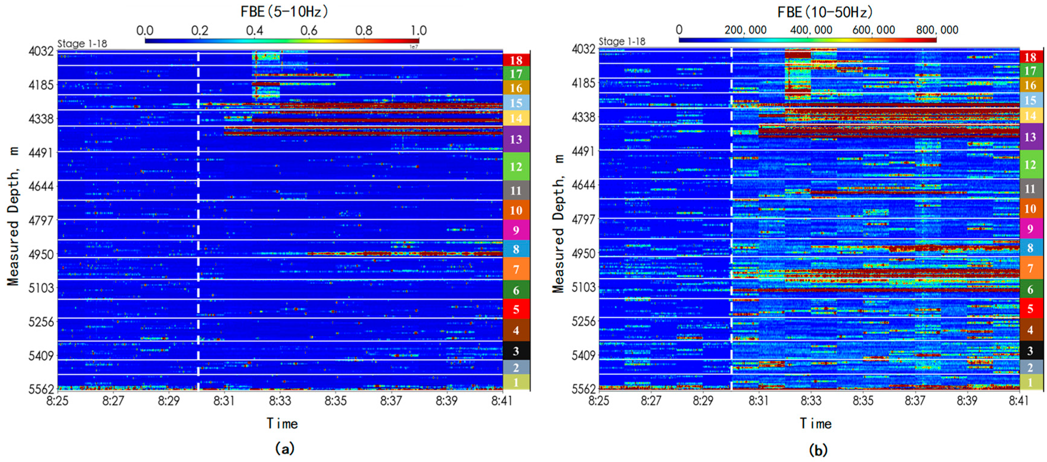
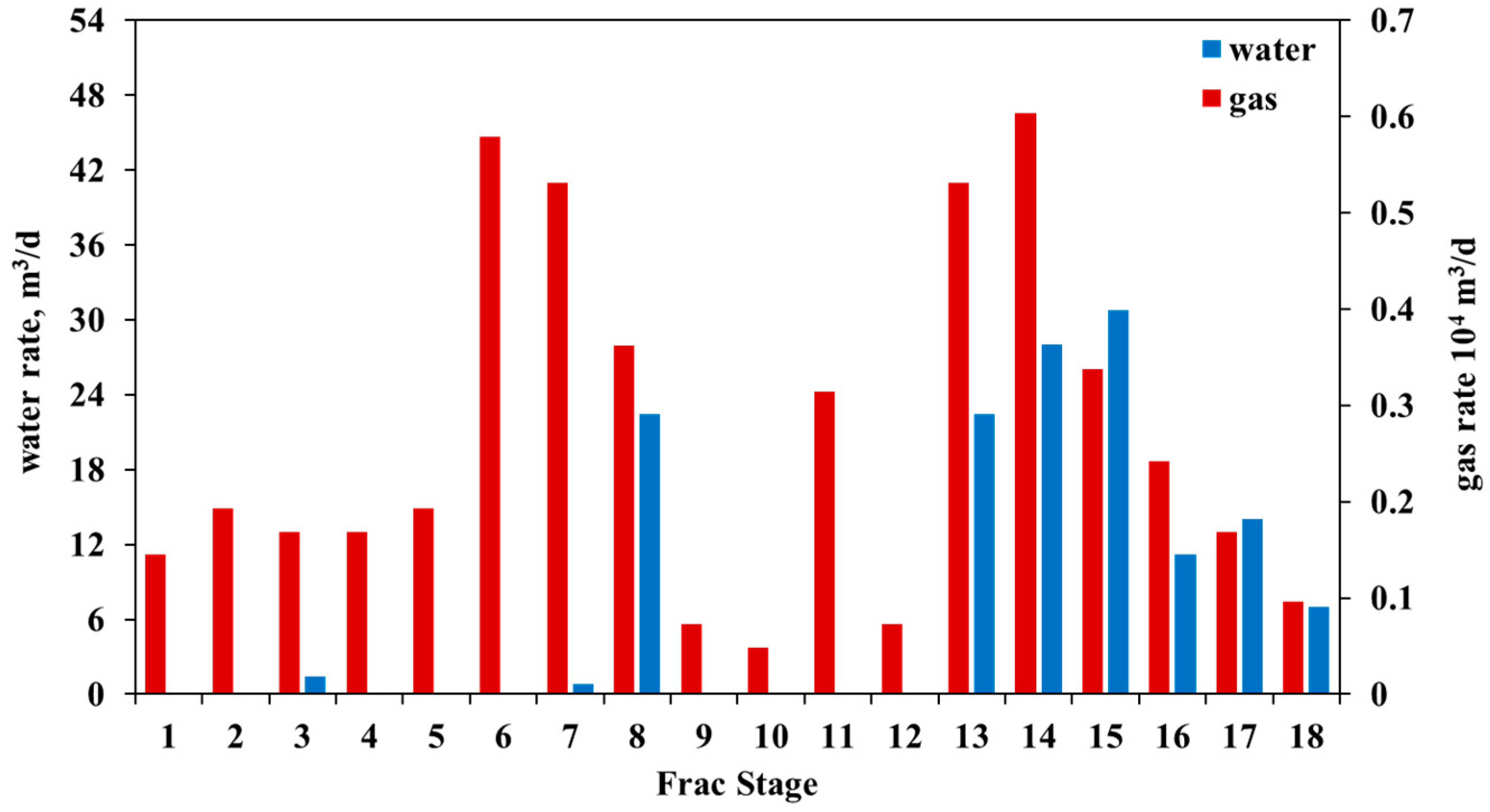
4.2. Production Profile Based on DAS Frequency Band Energy

The acoustic signal exhibits a linear relationship with fluid flow rate [28]:
log ( q 3 ) = A L SP + B
where q is the flow rate; LSP is the sound pressure level, which it can be substituted by the frequency band energy (FBE) from DAS; A and B are correlation parameters.
Due to the uncertainty of coefficients A and B, the application of this formula has limitations. This paper evaluates the production profile of the production well based on the linear relationship provided by this empirical formula, using the percentage of acoustic energy across different frequency bands. DAS data from the second day of shut-in and stable production periods, as shown in Figure 16, were selected for analysis. Based on the sensitive response frequency bands of each phase during gas–water two-phase flow given by numerical simulations, the original DAS data from the horizontal section of the production well were filtered to extract the acoustic energy spectra in the 5–10 Hz and 10–50 Hz bands. Figure 17 shows the energy spectra for the 5–10 Hz and 10–50 Hz bands, with white horizontal lines marking the boundaries of the 18 fracturing stages. The numbers on the rightmost side indicate the stage numbers, and the white dashed line represents the well opening time. It can be clearly observed that there is no significant acoustic energy during the shut-in phase, while noticeable energy response bands appear several minutes after the well is opened. In Figure 17a, stages 13–15 and stage 8 show consistently strong energy responses, while stages 15–18 have weaker responses, indicating water production from these stages. Compared to the 5–10 Hz range, Figure 17b shows energy responses across the entire horizontal section within the 10–50 Hz range, indicating gas production from all stages. Stages 6–8, stage 11, and stages 13–15 exhibit consistently strong energy responses, suggesting higher gas production in these stages.
The energy of a specific fracturing stage is represented by the cumulative energy across all channels with energy responses within that stage. The energy profile for each stage’s gas and water production rate is obtained by multiplying the ratio of the energy of that stage to the total energy of all responding stages by the surface daily water and gas flow rate. As shown in Figure 18, stages 13–18 correspond to continuous gas–water co-production stages. By utilizing the volume factors for gas (0.0039) and water (0.99), along with their respective surface flow rates, the downhole flow rates were calculated. The gas–water ratio was then determined based on the ratio of the downhole flow rates of gas and water (Figure 19). It can be observed that stages 13, 14, and 16 exhibit a relatively higher gas–water ratio (above 0.8), whereas stages 15, 18, and 19 show lower gas–water ratios (ranging from 0.4 to 0.6). Projecting the gas–water ratio for each stage onto the Mandhane flow pattern map (Figure 20), it was evident that the flow regimes were primarily within the stratified flow and bubble flow regions. From the toe side (stages 13, 14, 15) to the heel side (stages 16, 17, 18) of the horizontal well, the flow pattern transitioned from bubble flow to stratified flow. The following analysis focuses on the frequency range of acoustic amplitude peak responses for these six stages.

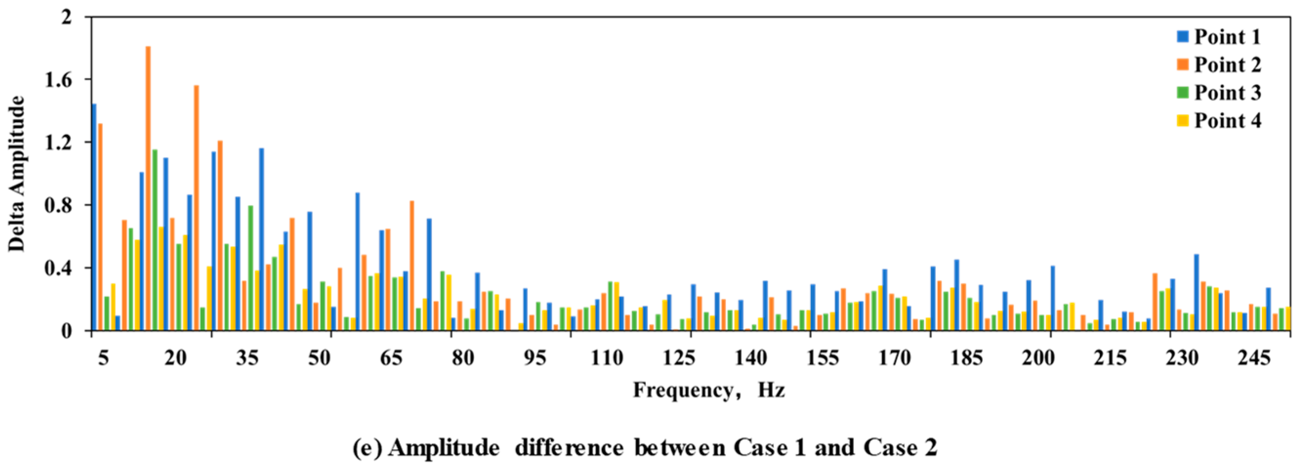
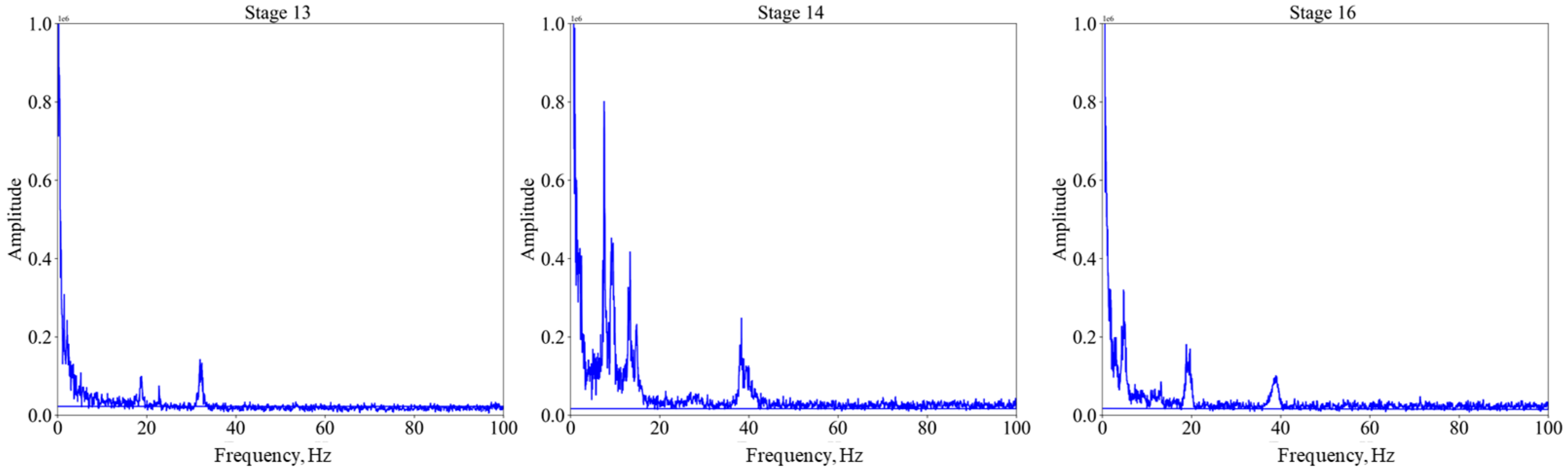
4.3. DAS Amplitude Response Frequency Band Analysis

Spectrum analysis converts time-domain signals into frequency-domain signals through Fourier transformation, allowing for the analysis of the signal’s frequency components. The analysis methods for time–frequency and spatial–frequency domains are essentially the same. By determining the frequency-domain coordinates, we can accurately locate the frequency components of the signal in the frequency domain and conduct the corresponding analysis. The formula to determine the frequency domain coordinates is
ft fs 2 : 0 : fs 2 ,
where ft is the frequency-domain coordinate and fs is the sampling frequency.
During spectrum analysis, we selected raw DAS acoustic amplitude data from the stable production period, focusing on perforations and their surrounding locations within the fracturing stage. The frequency was filtered to 200 Hz, with the frequency-domain coordinate ft converted to [−100 Hz:0:100 Hz]. Since the spectrum is symmetric, the coordinate of the frequency domain (ft) is shown as [0:100 Hz].
Figure 21 shows the amplitude response for stages 13, 14, and 16, which have higher gas–water ratios, within the 0–100 Hz range. It can be observed that all three stages exhibit amplitude peaks in the 5–50 Hz range, with stage 14 showing the highest and widest response peak, correlating with the highest gas production. Figure 22 also presents the amplitude response for the stages with lower gas–water ratios. Stages 17 and 18 exhibit peaks in the 5–10 Hz range, while stage 15 shows a relatively higher peak in the 10–25 Hz range, possibly due to its higher gas and water production. Comparatively, stages with higher gas–water ratios demonstrate a broader frequency range of amplitude response and higher peak amplitudes compared to stages with lower gas–water ratios. The results of DAS data analysis are consistent with numerical simulations, supporting the use of acoustic energy within the sensitive frequency bands for interpreting production profiles for gas and water separately.
The average gas–water ratio for stages 13, 14, and 16 is 0.88, nearly twice that of the average gas–water ratio for stages 15, 17, and 18. Based on the numerical simulation results, as the gas–water ratio increases, the frequency response range of the gas–water two-phase flow also broadens. For the three stages with higher gas–water ratios, amplitude peaks are observed around 20 Hz and 40 Hz. In contrast, the three stages with lower gas–water ratios exhibit amplitude peaks within the 5–25 Hz range. However, it can be observed that the three stages with higher gas–water ratios did not show an overall increase in amplitude across the 5–50 Hz range as predicted by the numerical simulations. This discrepancy may be attributed to the complex sources of noise present in the well, whereas the numerical simulation considered a single source of noise. The results of DAS data analysis are consistent with numerical simulations, supporting the use of acoustic energy within the sensitive frequency bands for interpreting production profiles for gas and water separately.

5. Conclusions

This study simulates the acoustic signals of fluid in the wellbore under different flow patterns and gas–water ratio conditions using a numerical model. The correlation among acoustic amplitude, the SPL, the frequency range of the acoustic response, and response location was analyzed. The acoustic response frequency range after increasing the gas–water ratio is validated using DAS data from an actual production well. The simulation results provide a reference range for frequency band selection during the analysis of DAS data from production wells, improving data processing efficiency. Based on the simulations results, high-frequency (>0.5 Hz) DAS data can be used for qualitative analysis of the gas–water ratio in the horizontal section of production wells, laying the foundation for future quantitative analysis between gas–water ratios and acoustic signals.
The main conclusions of this paper are as follows:
(1) By simulating acoustic signals of gas–water two-phase flow under different gas–water ratios for three flow patterns, it was found that the acoustic amplitude and SPL of the water phase primarily respond within the 5–10 Hz range, while the gas phase primarily responds within the 10–50 Hz range. The response intensity of the amplitude and the SPL during gas–water two-phase flow has a strong correlation with the observation location, with values increasing close to the fluid inlet as the gas–water ratio increases.
(2) Based on the numerical simulation results and the linear relationship between acoustic energy and flow rate, acoustic energy data in the 5–10 Hz and 10–50 Hz ranges were extracted from a shale gas production well to interpret the production profile of each stage.
(3) A frequency band analysis of the raw DAS amplitude data collected from a shale gas production well was conducted. The results showed that, compared to stages with lower gas–water ratios, those with higher gas–water ratios exhibited greater DAS amplitudes and broader frequency response ranges, consistent with the numerical simulation results.

Author Contributions

Conceptualization, Z.L. (Zhong Li) and W.S.; methodology, Y.W.; software, Y.Y.; validation, M.L.; formal analysis, J.J.; investigation, Z.L. (Zhenbo Li); resources, L.S.; data curation, H.G.; writing original draft preparation, Y.Y.; writing review and editing, H.G.; visualization, J.J.; supervision, Y.W.; project administration, Z.L. (Zhong Li); funding acquisition, M.L. All authors have read and agreed to the published version of the manuscript.

Funding

This research was funded by project titled ‘Research on Real-Time Monitoring Technology for Wellbore Integrity Based on Optical Parameters’ from CNOOC (China) Co., Ltd. Beijing Research Center. The project grant number is CCL2023RCPS0433RSN.

Institutional Review Board Statement

Not applicable.

Informed Consent Statement

Not applicable.

Data Availability Statement

The numerical simulation data in the paper can be obtained directly by contacting the corresponding author, Weibo Sui (suiweibo@cup.edu.cn), or the author, Huan Guo (2024310190@student.cup.edu.cn). However, the DAS data of the production well is confidential and cannot be disclosed.

Conflicts of Interest

The authors declare no conflict of interest.

References

  1. Cao, K.; Siddhamshetty, P.; Ahn, Y.; El-Halwagi, M.M.; Sang-Il Kwon, J. Evaluating the spatiotemporal variability of water recovery ratios of shale gas wells and their effects on shale gas development. J. Clean. Prod. 2020, 276, 123171. [Google Scholar] [CrossRef]
  2. Guo, M.; Lu, X.; Nielsen, C.P.; McElroy, M.B.; Shi, W.; Chen, Y.; Xu, Y. Prospects for shale gas production in China: Implications for water demand. Renew. Sustain. Energy Rev. 2016, 66, 742–750. [Google Scholar] [CrossRef]
  3. Mi, L. Inversion method of discrete fracture network of shale gas based on gas production profile. Acta Pet. Sin. 2021, 42, 481–491. [Google Scholar]
  4. Wei, P.; Dejia, D.; Jun, M.; Tongyi, Z.; Ying, H.; Shuang, A. Production Logging of Shale Gas Well in China. In Proceedings of the SPE Asia Pacific Hydraulic Fracturing Conference, Beijing, China, 24–26 August 2016. [Google Scholar]
  5. Basov, A.; Bukov, O.; Shevchuk, T.; Lazutkin, D.; Saprykina, K.; Kiselev, V.; Novikov, I.; Drobot, A. Confirmed Effectiveness of Tracers’ Production Logging in Comparison with Conventional Production Logging. In Proceedings of the SPE/IATMI Asia Pacific Oil & Gas Conference and Exhibition, Bali, Indonesia, 29–31 October 2019. [Google Scholar]
  6. Zhang, J.; Lan, W.; Deng, C.; Wei, F.; Luo, X. Thermal Optimization of High-Temperature Downhole Electronic Devices. IEEE Trans.Compon. Packag. Manuf. Technol. 2021, 11, 1816–1823. [Google Scholar] [CrossRef]
  7. Haustveit, K.; Haffener, J.; Young, S.; Dwyer, J.; Glaze, G.; Green, B.; Ketter, C.; Williams, T.; Brinkley, K.; Elliott, B. Cementing: The Good, the Bad, and the Isolated—Techniques to Measure Cement Quality and its Impact on Well Performance. In Proceedings of the SPE Hydraulic Fracturing Technology Conference and Exhibition, The Woodlands, TX, USA, 6–8 February 2024. [Google Scholar]
  8. Mahue, V.; Jimenez, E.; Dawson, P.; Trujillo, K.; Hull, R. Repeat DAS and DTS Production Logs on a Permanent Fiber Optic Cable for Evaluating Production Changes and Interference with Offset Wells. In Proceedings of the SPE/AAPG/SEG Unconventional Resources Technology Conference, Houston, TX, USA, 20–22 June 2022. [Google Scholar]
  9. Ugueto, G.; Wu, K.; Jin, G.; Zhang, Z.; Haffener, J.; Mojtaba, S.; Ratcliff, D.; Bohn, R.; Chavarria, A.; Wu, Y.; et al. A Catalogue of Fiber Optics Strain-Rate Fracture Driven Interactions. In Proceedings of the SPE Hydraulic Fracturing Technology Conference and Exhibition, The Woodlands, TX, USA, 31 January–2 February 2023. [Google Scholar]
  10. Cherubini, A.; Richard, S.; Jestin, C.; Calbris, G.; Lanticq, V. Real-Time Downhole Monitoring Using DAS and DTS: A New Technology for Leak Detection and Well Integrity. In Proceedings of the International Petroleum Technology Conference, Bangkok, Thailand, 1–3 March 2023. [Google Scholar]
  11. Sui, W.; Wen, C.; Sun, W.; Li, J.; Guo, H.; Yang, Y.; Song, J. Joint application of distributed optical fiber sensing technologies for hydraulic fracturing monitoring. Nat. Gas Ind. 2023, 43, 87–103. [Google Scholar]
  12. Wang, Y.; Wu, Z.; Wang, F. Research Progress of Applying Distributed Fiber Optic Measurement Technology in Hydraulic Fracturing and Production Monitoring. Energies 2022, 15, 7519. [Google Scholar] [CrossRef]
  13. Martinez, R.; Hill, A.D.; Zhu, D. Diagnosis of Fracture Flow Conditions with Acoustic Sensing. In Proceedings of the SPE Hydraulic Fracturing Technology Conference, The Woodlands, TX, USA, 4–6 February 2014. [Google Scholar]
  14. Budiansky, B.; Drucker, D.C.; Kino, G.S.; Rice, J.R. Pressure sensitivity of a clad optical fiber. Appl. Opt. 1979, 18, 4085–4088. [Google Scholar] [CrossRef] [PubMed]
  15. Jayaram, V.; Hull, R.; Wagner, J.; Zhang, S. Hydraulic Fracturing Stimulation Monitoring with Distributed Fiber Optic Sensing and Microseismic in the Permian Wolfcamp Shale Play. In Proceedings of the 7th Unconventional Resources Technology Conference, Denver, CO, USA, 22–24 July 2019. [Google Scholar]
  16. Pakhotina, J.; Zhu, D.; Hill, A.D. Evaluating Perforation Erosion and its Effect on Limited Entry by Distributed Acoustic Sensor DAS Monitoring. In Proceedings of the SPE Annual Technical Conference and Exhibition, Virtual, 26–29 October 2020. [Google Scholar]
  17. Li, X.; Zhang, J.; Grubert, M.; Laing, C.; Chavarria, A.; Cole, S.; Oukaci, Y. Distributed Acoustic and Temperature Sensing Applications for Hydraulic Fracture Diagnostics. In Proceedings of the SPE Hydraulic Fracturing Technology Conference and Exhibition, The Woodlands, TX, USA, 4–6 February 2020. [Google Scholar]
  18. In’t panhuis, P.; den Boer, H.; van der Horst, J.; Paleja, R.; Randell, D.; Joinson, D.; McIvor, P.; Green, K.; Bartlett, R. Flow Monitoring and Production Profiling Using DAS. In Proceedings of the SPE Annual Technical Conference and Exhibition, Amsterdam, The Netherlands, 27–29 October 2014. [Google Scholar]
  19. Bukhamsin, A.; Horne, R. Using Distributed Acoustic Sensors to Optimize Production in Intelligent Wells. In Proceedings of the SPE Annual Technical Conference and Exhibition, Amsterdam, The Netherlands, 27–29 October 2014. [Google Scholar]
  20. van der Horst, J.; Den Boer, H.; In’t Panhuis, P.; Wyker, B.; Kusters, R.; Mustafina, D.; Groen, L.; Bulushi, N.; Mjeni, R.; Awan, K.F.; et al. Fibre Optic Sensing For Improved Wellbore Production Surveillance. In Proceedings of the International Petroleum Technology Conference, Doha, Qatar, 19 January 2014. [Google Scholar]
  21. Moradi, P.; Seabrook, B.; Adair, N.; Garza, R. Resolving Multiphase Fractions in Horizontal Wells Using Speed of Sound Measured with Distributed Acoustic Sensors and a PVT Database. In Proceedings of the SPE/AAPG/SEG Unconventional Resources Technology Conference, Houston, TX, USA, 17–19 June 2024. [Google Scholar]
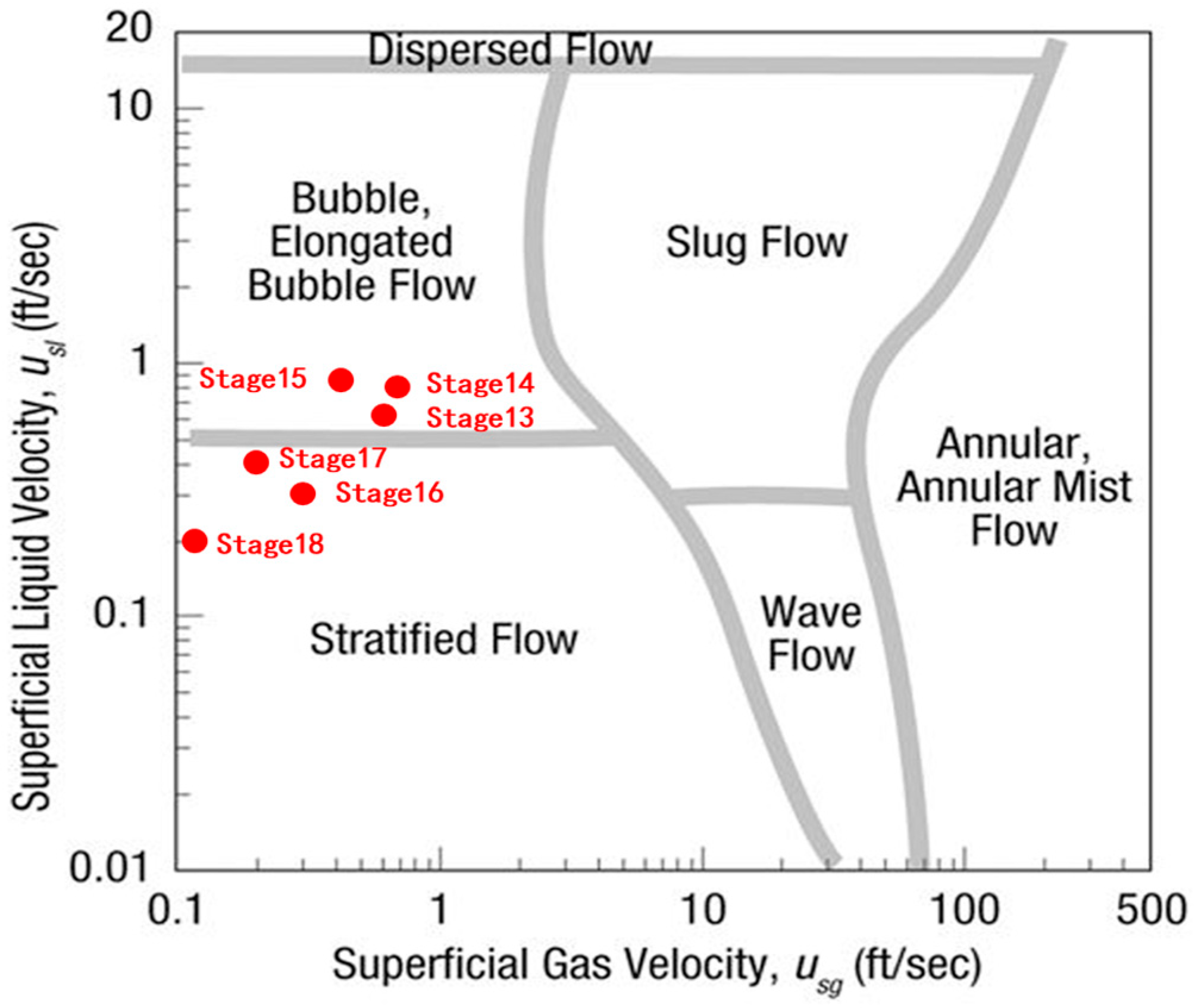
  22. Mandhane, J.M.; Gregory, G.A.; Aziz, K. A flow pattern map for gas—Liquid flow in horizontal pipes. Int. J. Multiph. Flow 1974, 1, 537–553. [Google Scholar] [CrossRef]
  23. Economides, M.J. Petroleum Production Systems; Prentice Hall: Hoboken, NJ, USA, 2013. [Google Scholar]
  24. Chen, J.; Chen, T. Petroleum Gas-Liquid Two-Phase Pipe Flow, 2nd ed.; Energy Science; Petroleum Industry Press: Beijing, China, 2010. (In Chinese) [Google Scholar]
  25. Lighthill, M.J. On sound generated aerodynamically I. General theory. Proceedings of the Royal Society of London. Ser. A. Math. Phys. Sci. 1952, 211, 564–587. [Google Scholar]
  26. Williams, B.J.E.F.; Hawkingst, D.L. Sound generation by turbulence and surfaces in arbitrary motion. Philos. Trans. R. Soc. Lond. Ser. A Math. Phys. Sci. 1969, 264, 321–342. [Google Scholar]
  27. Jianrong, W.; Spek, A.v.d.; Georgi, D.T.; Chace, D.M. Characterizing Sound Generated by Multiphase Flow. In Proceedings of the SPE Annual Technical Conference and Exhibition, Houston, TX, USA, 3–6 October 1999. [Google Scholar]
  28. Sakaida, S.; Pakhotina, I.; Zhu, D.; Hill, A.D. Estimation of Fracture Properties by Combining DAS and DTS Measurements. In Proceedings of the SPE International Hydraulic Fracturing Technology Conference & Exhibition, Muscat, Oman, 11–13 January 2022. [Google Scholar]
Figure 1. Schematic of wellbore fluid flow measurement utilizing fiber optics.
Photonics 11 01049 g001
Figure 2. Mandhane flow pattern diagram [23].
Photonics 11 01049 g002
Figure 3. Steady one-dimensional split-phase flow [24].
Photonics 11 01049 g003
Figure 4. Schematic diagram of horizontal pipe geometry model.
Photonics 11 01049 g004
Figure 5. Observation points in simulation of sound field.
Photonics 11 01049 g005
Figure 6. Gas-phase volume fraction distribution.
Photonics 11 01049 g006
Figure 7. The corresponding position of each case on the Mandhane flow pattern map.
Photonics 11 01049 g007
Figure 8. The simulated velocity distribution in the horizontal pipe for the six cases.
Photonics 11 01049 g008
Figure 9. The simulated pressure distribution in the horizontal pipe for the six cases.
Photonics 11 01049 g009
Figure 10. Acoustic simulation results with different frequencies.
Photonics 11 01049 g010
Figure 11. SPL distribution with different frequencies in the six cases.
Photonics 11 01049 g011
Figure 12. Mean SPL at different locations in the six cases.
Photonics 11 01049 g012
Figure 13. Relationship between sound amplitude, SPL, and frequency for bubbly flow (Case 1 and Case 2).
Photonics 11 01049 g013aPhotonics 11 01049 g013b
Figure 14. Relationship between amplitude, SPL, and frequency for slug flow (Case 3 and Case 4).
Photonics 11 01049 g014
Figure 15. Relationship between amplitude, SPL, and frequency for stratified flow (Case 5 and Case 6).
Photonics 11 01049 g015
Figure 16. Surface production data before and after DAS monitoring.
Photonics 11 01049 g016
Figure 17. Frequency band energy of production well: (a) 5–10 Hz; (b) 10–50 Hz.
Photonics 11 01049 g017
Figure 18. The production profile of the production well.
Photonics 11 01049 g018
Figure 19. Gas–water ratio for stage 13 to stage 18.
Photonics 11 01049 g019
Figure 20. The corresponding position of each stage on the Mandhane flow pattern map.
Photonics 11 01049 g020
Figure 21. Amplitude response for stages with higher gas–water ratios.
Photonics 11 01049 g021
Figure 22. Amplitude response for stages with lower gas–water ratios.
Photonics 11 01049 g022
Table 1. Input parameters of each modeling case.
Case NumberGas Velocity
(m/s)
Water Velocity
(m/s)
Gas–Water
Ratio
Gas Surface
Flow Rate
(104 m3/d)
Water Surface Flow Rate (m3/d)
10.220.12.9864
20.30.60.54.3260
31.51.5121.6650
431343.2430
50.20.0452.918
60.60.06108.626
Disclaimer/Publisher’s Note: The statements, opinions and data contained in all publications are solely those of the individual author(s) and contributor(s) and not of MDPI and/or the editor(s). MDPI and/or the editor(s) disclaim responsibility for any injury to people or property resulting from any ideas, methods, instructions or products referred to in the content.

