Multiplet Network for One-Shot Mixture Raman Spectrum Identification

Abstract

Raman spectroscopy is widely used for material identification, but mixture analysis remains challenging due to noise and fluorescence interference. To tackle this issue, we propose the Multiplet Network, an advanced deep-learning model specifically designed for identifying components in mixtures. This model employs a shared-weight residual network to map both mixture and candidate spectra into a unified feature space, where least-squares regression is utilized to predict the components. Our framework enhances feature extraction and component identification capabilities, outperforming traditional regression methods. Experimental evaluations on the RRUFF dataset showed that our model achieved superior accuracy, especially as the number of candidate spectra increased. Furthermore, it exhibited remarkable robustness against Gaussian noise and baseline variations, maintaining high accuracy under challenging conditions. To assess the real-world applicability, the model was tested on experimentally collected mixture spectra with significant noise and baseline shifts. The results confirmed that it effectively identified major components under complex spectral conditions. Additionally, the unique structure of the model’s feature extraction combined with least squares allowed it to handle varying sizes of spectral libraries, ensuring both flexibility and scalability. Overall, our approach provides a robust and adaptable solution for Raman mixture analysis, with strong potential for complex chemical and material identification in practical applications.

1. Introduction

Raman spectroscopy is a powerful analytical technique that extracts vibrational information from molecules and is commonly used as a fingerprinting technique for identifying sample components. It offers advantages such as rapid analysis, non-destructiveness, and no need for sample preparation, making it widely applicable for unknown material identification across fields such as environmental monitoring [1,2], forensics [3], pharmaceutical screening [4], food safety [5], and public safety [6]. Various methods have been developed for Raman spectral identification, including spectral matching [7,8,9] and deep neural networks (DNNs) [10,11,12]. While these approaches perform well for identifying single-component spectra, challenges remain in recognizing components in mixtures due to spectral overlap and noise interference. To address this challenge, researchers have developed several approaches, such as Spectral Search [13], reverse searching [14], non-negative least squares (NNLS) [14,15], and non-negative elastic nets (NNEN) [16]. Least squares (LS) [17] fits the mixture component coefficients by minimizing the sum of squared residuals, but its results may include negative values, which is unreasonable in spectral analysis. To address this issue, NNLS introduces a non-negativity constraint on top of LS to ensure that the fitted results remain non-negative. However, NNLS is prone to overfitting when handling high-dimensional data. To mitigate this, NNEN combines L1 regularization and L2 regularization while enforcing the non-negativity constraint, effectively reducing the risk of overfitting. However, NNEN remains a linear model, and its performance is limited by the quality of the input features, making it difficult to capture complex nonlinear relationships. Most of these methods rely on spectral similarity or distance metrics. Additionally, they often require extensive spectral preprocessing, including smoothing, denoising, baseline correction, and peak detection, which significantly impact recognition outcomes.

With the advancement of deep learning, DNN-based methods have gained increasing attention for mixture Raman spectrum identification. For instance, Fan et al. [18] proposed deep learning-based component identification (DeepCID), a CNN-based model that predicts the presence of components in mixtures and outperforms traditional methods. However, DeepCID requires training a separate CNN model for each compound in the database, ignoring inter-component relationships and resulting in high computational costs and inefficiencies. To overcome this limitation, Fan et al. introduced DeepRaman [19], which can be applied across different datasets without retraining or transfer learning. DeepRaman employs a Pseudo-Siamese neural network (PSNN) [20] to estimate the similarity between an unknown sample and all candidate spectra in the database, followed by a non-negative elastic net [16] for final component determination. However, if the PSNN fails to select the correct candidate spectra, the final prediction is compromised, and the non-negative elastic net may become the performance bottleneck.

Other significant advancements in the field include ConInceDeep by Zhao et al. [21], which leverages wavelet transforms for feature extraction in complex mixtures, thereby enhancing the accuracy of Raman spectral identification; RamanFormer by Onur Can Koyun et al. [22], which integrates self-attention mechanisms for component recognition and quantification; a novel multi-label DNN by Pan et al. [23] for the identification of palm oil composition; and the cloud-network-end architecture presented by Liang et al. [24], which enables rapid mixture Raman spectral identification using deep learning techniques. Traditional DNNs often rely on large-scale mixed spectra to accurately learn the linear combination coefficients of components. However, in one-shot scenarios, where only a single reference spectrum per class is available, directly training DNNs can lead to overfitting. Additionally, trained DNN models are typically limited to specific databases and require retraining for new datasets, limiting their practical applicability.

To overcome these limitations, this study proposes a Multiplet Network (MN) for component identification in mixtures in Raman spectra. This method is database-independent, eliminating the need for retraining and making it a generalizable solution for mixture Raman spectral recognition. It maintains superior performance even in one-shot scenarios. The Multiplet Network accepts multiple inputs, including the mixture spectrum and all candidate spectra from the database, with shared weights across networks. It efficiently extracts Raman spectral features and applies least-squares regression on the embedded vectors to predict component labels. The performance of the Multiplet Network was evaluated using both simulated mixture datasets from the RRUFF database [25] and experimentally collected mixture spectra, demonstrating outstanding accuracy, adaptability to new datasets, and robust generalization capabilities. The Multiplet Network method provides a versatile and reliable solution for component recognition in complex mixtures of Raman spectra, overcoming previous limitations and challenges.

2. Materials and Methods

2.1. Dataset

(1)

RRUFF Dataset. We utilized data from the RRUFF database (https://rruff.info/, accessed on 16 May 2024) as the source for our training dataset. Developed by Professor Robert Downs at Arizona State University in 2006, this database offers a comprehensive collection of mineral Raman spectra with varying quality. From this database, we selected three datasets, ‘excellent_oriented’, ‘excellent_unoriented’, and ‘unrated_oriented’, comprising 16,998 spectra across 1723 classes. To align with the model’s input requirements, all spectra were interpolated or resampled to a length of 256. The procedure for generating the training spectra was as follows:

Step 1: Randomly select one spectrum from each of the 10 categories in the RRUFF database to form a candidate spectral library, $\mathbf{S}=[{\mathbf{s}}_1,{\mathbf{s}}_2,\dots ,{\mathbf{s}}_{10}]$.

Step 2: Randomly generate a corresponding coefficient vector, $\mathbf{A}$, for the candidate library $\mathbf{S}$, with the dimensions (10,1). The number of non-zero values in $\mathbf{A}$ is between 1 and 3, corresponding to a univariate mixture (pure substance), a binary mixture, or a ternary mixture.

Step 3: Compute the mixture spectrum ${\mathbf{S}}_{\mathrm{mix}}=\mathbf{A}\mathbf{S}+ϵ$, where $ϵ$ is the simulated random noise and fluorescence background noise, and concatenate ${\mathbf{S}}_{\mathrm{mix}}$ with $\mathbf{S}$ to form a Multiplet. The Multiplet is an array of the size (11,256), which serves as the input data for training. Denote this as $X=[{\mathbf{S}}_{\mathrm{mix}},{\mathbf{s}}_1,{\mathbf{s}}_2,\dots ,{\mathbf{s}}_{10}]$. The coefficient vector $\mathbf{A}$ serves as the label for the training data.

Steps 1 through to 3 are repeated to generate a total of $2\times {10}^6$ Multiplets as training samples.

(2)

Experimental Dataset. The Experimental Dataset included the Raman spectra of 28 common organic and inorganic compounds, such as urea and sodium urate, as well as their mixtures. These spectra were acquired using a self-built transmission Raman spectrometer. The dataset was divided into two parts: (1) the Raman spectra of 28 pure compounds, which served as the candidate spectral library, and (2) the Raman spectra of 9 mixtures, which were used as the test set. All spectra had a resolution of 7 cm⁻¹ and covered a wavenumber range of 200–2000 cm⁻¹. The spectra were acquired using an excitation wavelength of 785 nm with an excitation power of 300 mW. The integration time was adjusted between 1 and 10 s based on the Raman scattering intensity of different materials.

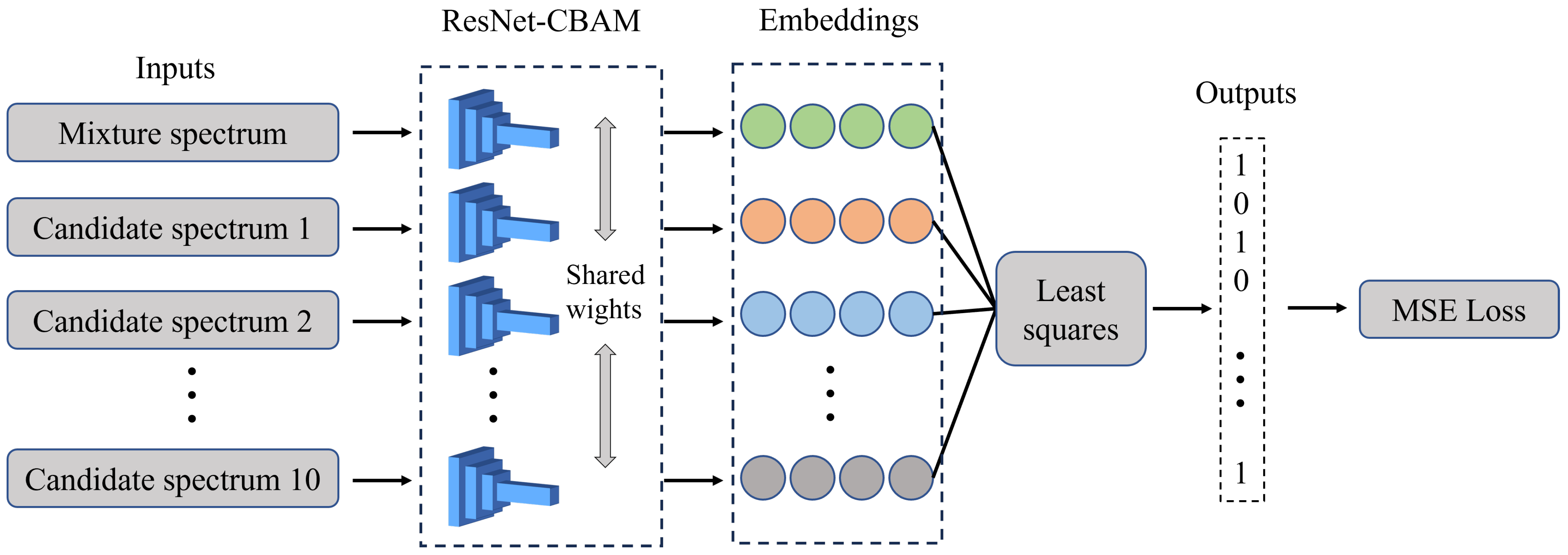
2.2. Multiplet Network

2.2.1. Mathematical Foundations of Mixture Decomposition

The Multiplet Network framework addresses the challenge of identifying chemical components within a mixture Raman spectrum by combining spectral decomposition theory with deep learning. At its core, the problem involves resolving a mixture spectrum, ${\mathbf{S}}_{\mathrm{mix}}$, into contributions from a predefined library of candidate spectral library, $\mathbf{S}=[{\mathbf{s}}_1,{\mathbf{s}}_2,\dots ,{\mathbf{s}}_{10}]$, where each ${\mathbf{s}}_i$ represents the spectrum of a pure substance. The mixture is modeled as a linear combination of these candidate spectral library:

$${\mathbf{S}}_{\mathrm{mix}}=a_1{\mathbf{s}}_1+a_2{\mathbf{s}}_2+\cdots +a_{10}{\mathbf{s}}_{10}=\mathbf{A}·\mathbf{S}$$

where $\mathbf{A}=[a_1,a_2,\dots ,a_{10}]$ encodes the contribution coefficients of each component. In an idealized scenario without noise or interference, solving for $\mathbf{A}$ reduces to a straightforward least-squares problem. By minimizing the reconstruction error $E=\parallel {\mathbf{S}}_{\mathrm{mix}}{-\mathbf{A}·\mathbf{S}\parallel }_2^2$, the coefficients can be calculated directly:

$$\mathbf{A}={\left({\mathbf{S}}^T\mathbf{S}\right)}^{-1}{\mathbf{S}}^T{\mathbf{S}}_{\mathrm{mix}}$$

However, real-world Raman spectra often contain noise, baseline drift, and nonlinear interactions between overlapping peaks, rendering this simplistic approach ineffective. To overcome these limitations, we introduce a learnable feature extraction step using a residual network $f_{\theta }$. This network maps raw spectral data into a latent space where noise is suppressed and discriminative features are emphasized. Specifically, the mixture spectrum and each candidate spectrum are transformed as follows:

$${\mathbf{R}}_{\mathrm{mix}}=f_{\theta }\left({\mathbf{S}}_{\mathrm{mix}}\right),{\mathbf{r}}_i=f_{\theta }\left({\mathbf{s}}_i\right),\mathbf{R}=[{\mathbf{r}}_1,{\mathbf{r}}_2,\dots ,{\mathbf{r}}_{10}]$$

Here, ${\mathbf{R}}_{\mathrm{mix}}$ and $\mathbf{R}$ represent the feature-space projections of the mixture and candidate spectral library, respectively. The coefficient vector $\mathbf{A}$ is then recalculated in this latent space using a modified least-squares formulation:

$$\mathbf{A}={\left({\mathbf{R}}^T\mathbf{R}\right)}^{-1}{\mathbf{R}}^T{\mathbf{R}}_{\mathrm{mix}}$$

By operating in the feature space, the model effectively disentangles overlapping spectral signatures and reduces sensitivity to noise. The training process leverages supervised learning with labeled pairs. Unlike conventional approaches that use fully connected layers to directly predict coefficients, our design decouples feature learning from coefficient estimation. This separation allows the model to generalize to libraries of varying sizes; for instance, it adapts seamlessly when the candidate library contains more or fewer than 10 components. The residual network $f_{\theta }$ is optimized to produce features that satisfy the linear mixture assumption, effectively acting as an adaptive filter that enhances the robustness of the decomposition.

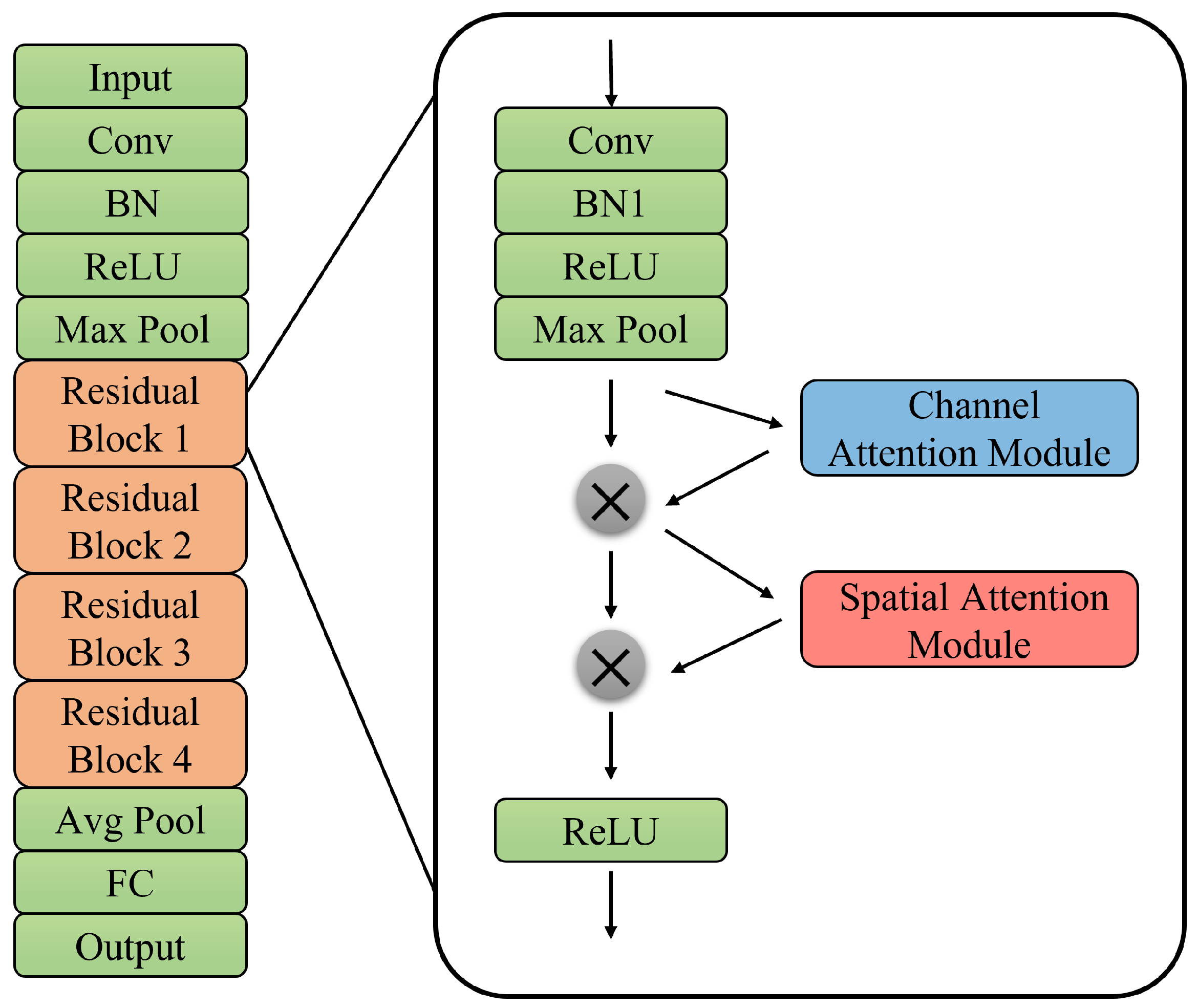
2.2.2. Network Architecture

A novel Multiplet Network is proposed for the component identification of mixtures. This network incorporates a structure similar to Siamese [20] and Triplet networks [26]. A Siamese network is a weight-shared, dual-branch neural network primarily designed to compare the similarity between two inputs. By using a shared feature extractor, the Siamese network ensures that different input spectra are mapped to the same feature space, allowing the calculation of their distance or similarity. The Triplet network further extends the Siamese network by using a Triplet input (Anchor, Positive, Negative), where the Anchor represents a candidate sample, the Positive represents a sample similar to the Anchor, and the Negative represents a sample dissimilar to the Anchor. The Triplet network optimizes the feature space distribution via the Triplet Loss Function, ensuring that the feature distance between similar samples is minimized and the distance between dissimilar samples is maximized.

The proposed Multiplet Network is a weight-shared, multi-branch neural network, where the input consists of a Multiplet (Query, candidate library). The Query represents the spectrum of the mixture, and the candidate library is a collection of spectra from pure substances, which are potential components of the mixture. The core objective of the model is to train an embedding network that effectively extracts spectral features so that the mappings of mixture spectra and candidate spectral library in the feature space better reflect their linear relationships with component labels. Through the weight-shared multi-branch architecture, both the mixture spectrum and spectra from the candidate library are projected into a unified feature space, and the component coefficients are directly computed using least squares. After obtaining the component coefficients, the network introduces a label-based loss function (Root Mean Square Loss, RMSLoss) to directly optimize the matching between the output component coefficients and the true component labels. As shown in Figure 1, the proposed Multiplet Network consists of 11 branch networks, with one branch dedicated to extracting characteristics from the mixture spectrum and the remaining 10 branches used to extract features from each pure substance in the candidate library. The number of branch networks is determined by the size of the candidate library.

The branch network is a ResNet [27] integrated with the Convolutional Block Attention Module (ResNet-CBAM), accepting a spectral sequence of the size (1, 256) as the input and outputting a feature vector of the size (1, 128). ResNet is a deep convolutional neural network (CNN) [28] architecture that addresses the vanishing gradient problem through residual connections, enabling the training of deeper and more stable networks. To enhance the model’s ability to capture important spectral features, we introduce the Convolutional Block Attention Module (CBAM) [29] into a 1D-ResNet10 architecture. As shown in Figure 2, the channel attention module [30] is added after the initial convolutional block and before the first residual block, while the spatial attention module [29] is integrated immediately after the channel attention module. The channel attention mechanism dynamically adjusts the weights of feature channels, emphasizing informative channels and suppressing less relevant ones. Meanwhile, the spatial attention mechanism focuses on the most significant regions of the spectral sequence by assigning higher weights to regions with notable variations. These attention mechanisms enable the model to adaptively extract and improve key features from input spectral data, improving its robustness and accuracy in complex tasks such as identifying mixture components.

After least-squares analysis, the coefficient vector is obtained, followed by binarization using a threshold determined through grid search to find the optimal value. This process generates the predicted vector, where 0 indicates that the component is absent from the mixture and 1 indicates that the component is present. The model was built using the PyTorch framework [31] and trained on a single NVIDIA 2080 Super GPU, with a total training time of 20 h.

2.3. Performance Evaluation

We evaluated the model’s performance in identifying mixture components using accuracy and the Jaccard Score [32,33]. Accuracy is defined as the proportion of samples for which the predicted labels exactly match the true labels, as given by the following formula:

$$\mathrm{Accuracy}={\displaystyle \frac{{\sum }_{i=1}^N\delta \left({\widehat{y}}_i,y_i\right)}{N}}$$

(1)

where N is the total number of samples, $y_i$ is the true label of the i-th sample, ${\widehat{y}}_i$ is the predicted label of the i-th sample, and $\delta$ is the indicator function, which takes a value of 1 if ${\widehat{y}}_i=y_i$ (exact match) and 0 otherwise. This stringent definition considers a sample accurately classified only when all of its sub-labels are correctly predicted. This definition ignores partial matches of labels, which may result in lower accuracy when dealing with sparse label sets. Therefore, we also used the Jaccard Score to assess the model’s performance. The Jaccard Score is based on the ratio of the intersection to the union of the predicted and true labels, which can be expressed by the following formula:

$$\mathrm{Jaccard}\mathrm{Score}={\displaystyle \frac{1}{N}}\sum _{i=1}^N{\displaystyle \frac{\left|{\widehat{y}}_i\cap y_i\right|}{\left|{\widehat{y}}_i\cup y_i\right|}}$$

(2)

where N is the total number of samples, ${\widehat{y}}_i\cap y_i$ is the number of sub-labels in the intersection of the predicted and true labels, and ${\widehat{y}}_i\cup y_i$ is the number of sub-labels in the union of the predicted and true labels. The Jaccard Score allows partial matching (only some labels are correctly predicted), making it more flexible and suitable for multi-label and sparse-label scenarios.

3. Results

Based on the RRUFF dataset, we generated $2\times {10}^6$ Multiplets as training data using the method described in Section 2.1, and the component coefficients of the mixtures were binarized to serve as labels. To ensure the model’s generalization performance and its ability to perform well on unseen datasets, we divided the RRUFF dataset into two subsets based on categories, one for training and one for testing. That is, the spectral categories used in the test set were completely different from those in the training set, which could be regarded as a completely new dataset. To further validate the practicality of the model, we also tested the model’s performance on the Experimental Dataset. During training, we used the Adam optimizer for weight updates, with an initial learning rate set to 0.001, and an exponential decay strategy, reducing the learning rate to 0.1 of the original value every 10 epochs. The batch size was set to 500, with a total of 50 training epochs, while monitoring the validation loss. If the validation loss did not decrease over five consecutive epochs, training was terminated early.

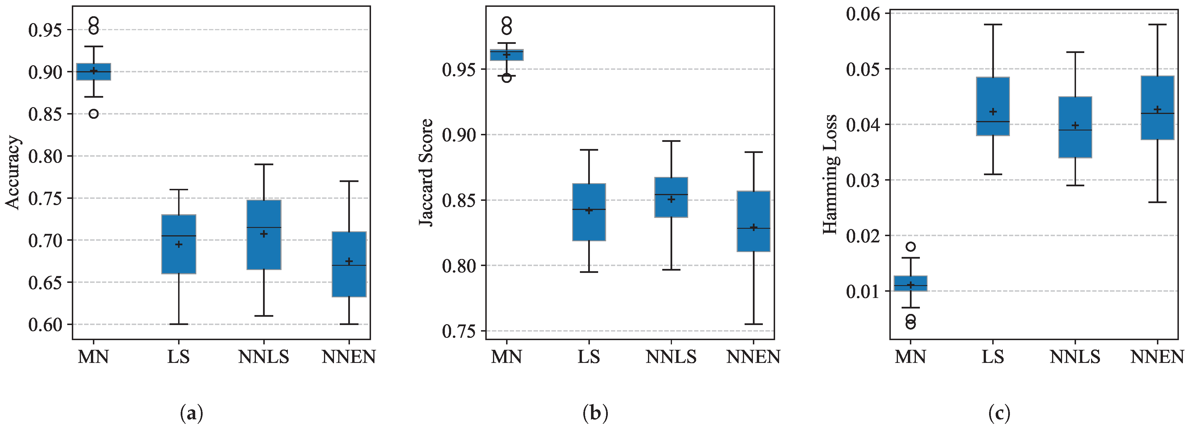
3.1. Performance on the RRUFF Dataset

For the RRUFF dataset, we designed a one-shot mixture identification experiment, treating the candidate spectral library as the support set within a few-shot learning framework. Both the candidate spectra and the spectra of an unknown mixture were fed into the model, which subsequently predicted the component labels of the mixture. As illustrated in Figure 3, we evaluated the overall performance of the model on the mixture component identification task using accuracy, the Jaccard Score, and Hamming Loss [34]. We also compared our approach against conventional methods, including LS, NNLS, and NNEN. The experimental results demonstrated that our proposed model outperformed traditional methods in terms of both accuracy and the Jaccard Score, with a particularly significant improvement in the Jaccard Score. This improvement highlighted the effectiveness of the feature extraction network in decomposing mixture spectra.

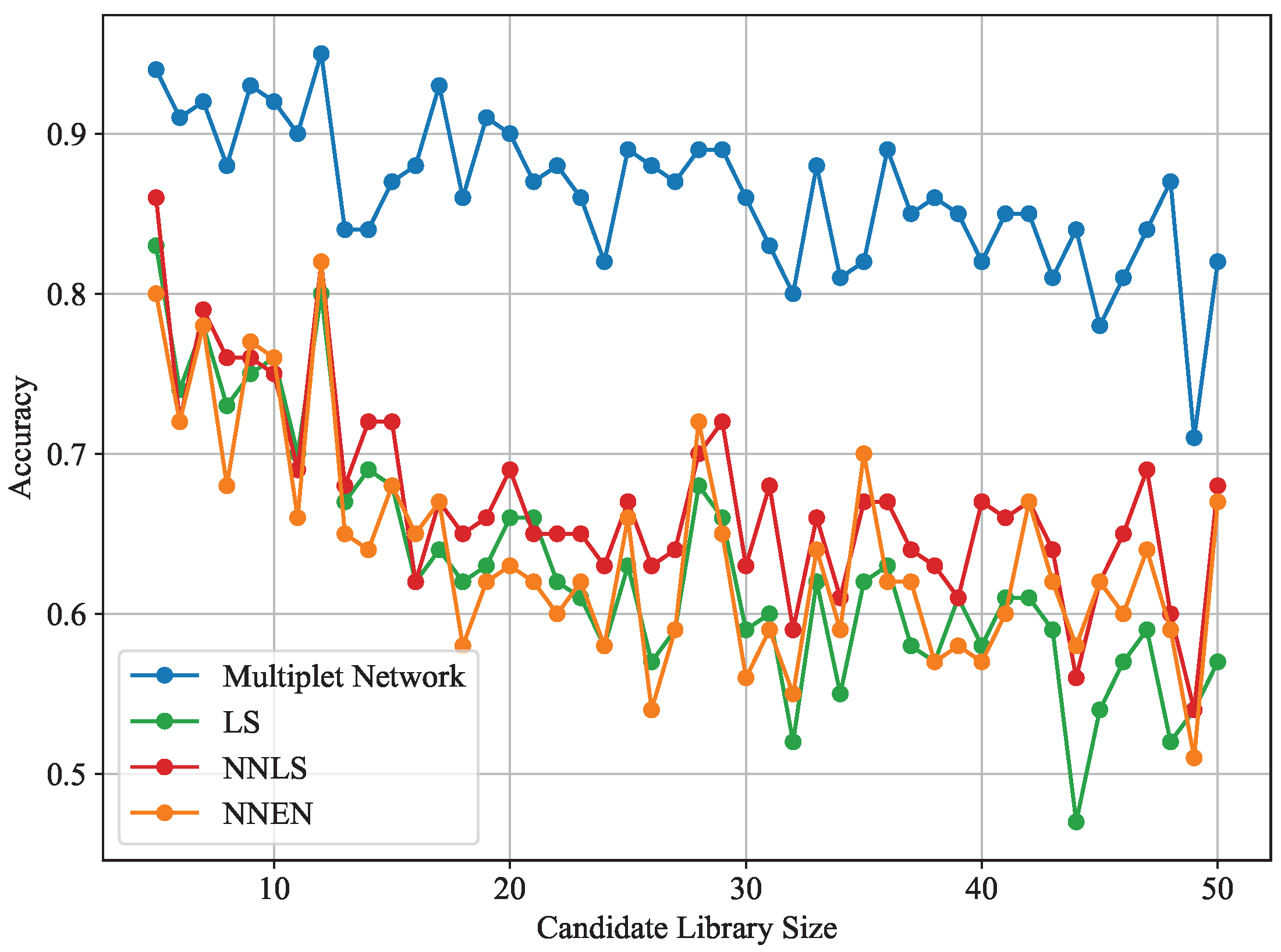
3.2. Impact of Support Set Size

Increasing the number of candidate spectra effectively broadened the possible combination space of spectral compositions. This expansion required the feature extraction network to distinguish spectral characteristics within an enlarged space, increasing the learning difficulty. Higher similarity among different spectra, particularly when specific components exhibited highly overlapping distributions in the feature space, reduced the model’s discriminative ability. To evaluate the model’s performance with a larger candidate spectral library, we analyzed the accuracy trend as a function of the support set size and compared it with those of traditional methods. As depicted in Figure 4, the accuracy of all methods decreased as the support set size increased. Nevertheless, our proposed model maintained a leading accuracy advantage even with a larger support set. This suggests that our model was more effective at extracting useful features from a large number of candidate spectra, mitigating the negative impact of information overload, and maintaining stable component identification performance despite the presence of redundant or noisy information.

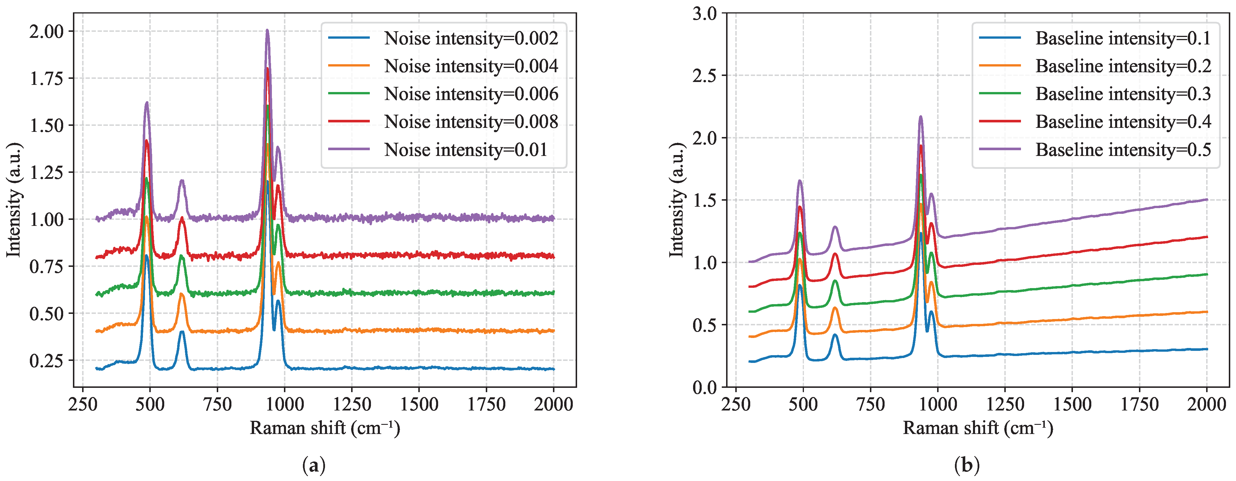
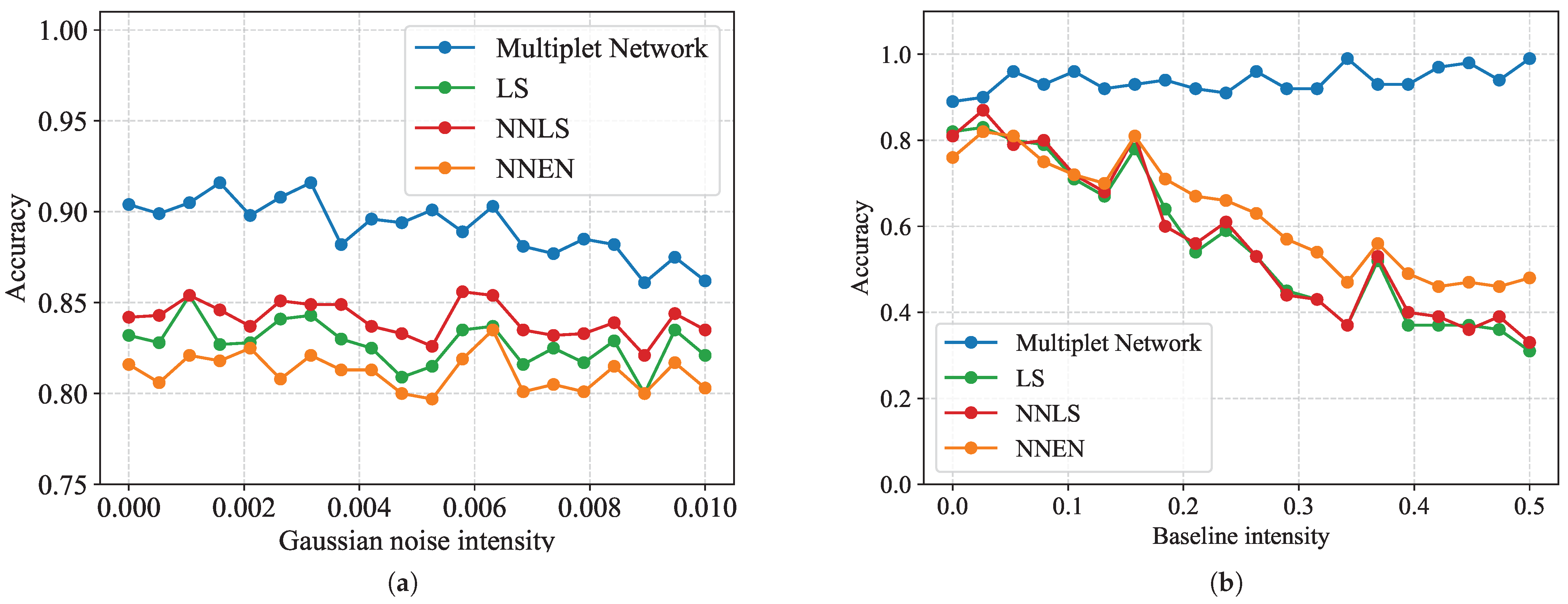
3.3. Robustness to Noise and Baseline Interference

Traditional regression methods, such as least-squares and non-negative least-squares regression, are susceptible to noise and spectral baseline variations in mixture component identification. To assess the robustness of different models under noise and baseline interference, we introduced Gaussian noise and a linear baseline to the spectra being tested (as shown in Figure 5) and evaluated the accuracy variations under different noise levels and baseline shifts. As shown in Figure 6a, while the traditional methods maintained stable accuracy in the presence of Gaussian noise, demonstrating relatively strong noise resistance, this was primarily because Gaussian noise is typically randomly distributed and its impact is spread across different spectral bands. Nevertheless, our proposed model still achieved superior performance under high-noise conditions. Figure 6b illustrates that when linear baseline interference was introduced, the performance of the traditional regression methods deteriorated significantly. In contrast, our model exhibited greater robustness against baseline shifts, maintaining higher accuracy and outperforming traditional methods. This indicated that our model could more effectively extract meaningful spectral features from noisy and baseline-shifted spectra, enhancing its adaptability in complex experimental environments. By leveraging a more powerful feature representation capability, our model could automatically filter out background interference and noise, thereby maintaining stable performance and reliable component identification.

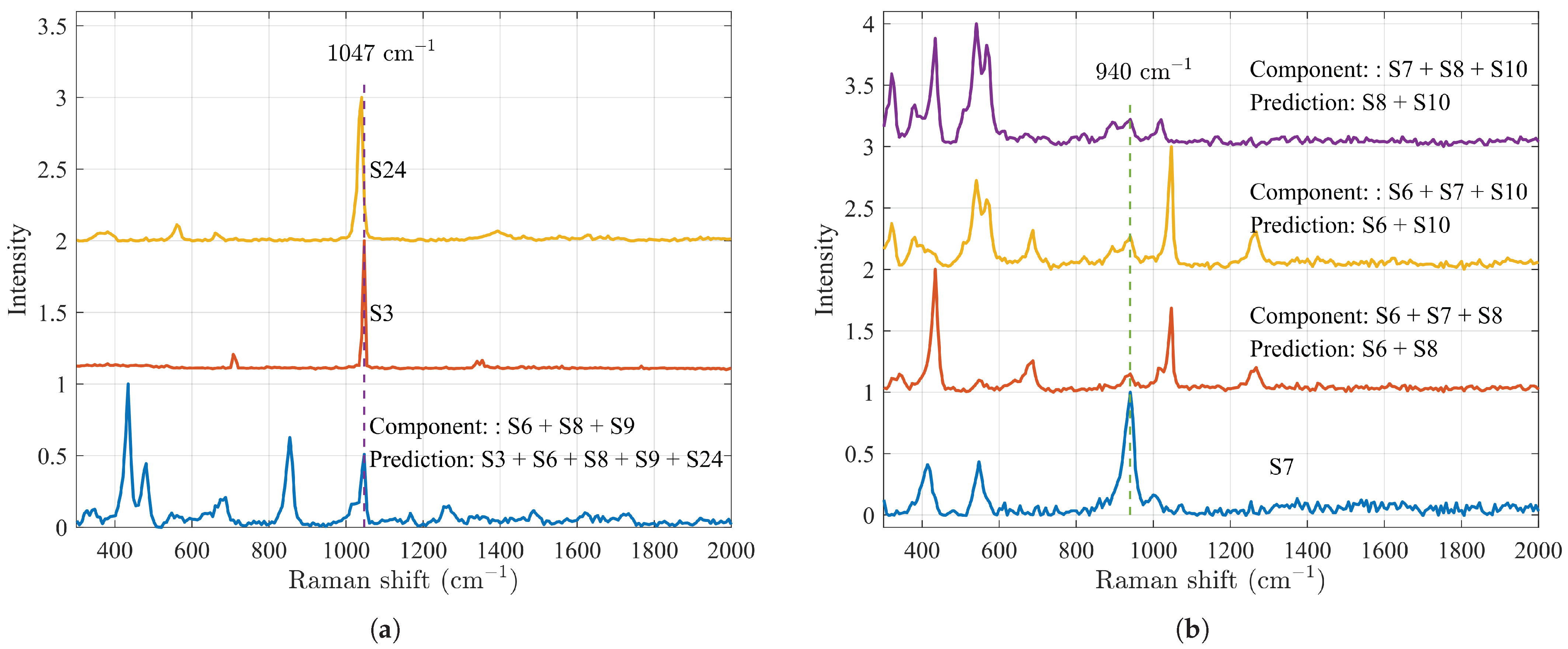
3.4. Performance on Real-World Mixtures

To evaluate the applicability of the model in real-world scenarios, we conducted a performance assessment using experimentally collected spectra of real mixture samples. Compared to the RRUFF dataset, the Experimental Dataset exhibited lower spectral quality, with increased noise, baseline drift, and other non-ideal factors. Moreover, the distribution and proportion of mixture components better reflected practical conditions, providing a more realistic evaluation of the model’s practicality and robustness.

The test mixtures consisted of two types: one set of binary and ternary mixtures obtained through powder blending and another set generated by linearly combining experimentally acquired pure-substance spectra to simulate binary and ternary mixtures. To better approximate real measurement conditions, Gaussian noise and baseline variations were added to the simulated mixtures.

Table 1. The identification results of nine powder mixtures, with a candidate library consisting of spectra from 28 compounds. The confidence represents the probability of the component being present in the mixture.

True Components	Predicted Components	Confidence	Jaccard Score
S1, S3, S5	S1, S5	[0.89, 0.67]	0.67
S1, S3	S1, S3	[0.69, 0.75]	1.00
S2, S5	S2, S5	[0.84, 0.56]	1.00
S4, S5	S4, S5	[0.87, 0.88]	1.00
S1, S5	S1, S5	[0.94, 0.66]	1.00
S6, S7, S8	S6, S8	[0.69, 1.07]	0.67
S6, S7, S10	S6, S10	[0.89, 0.86]	0.67
S6, S8, S9	S3, S6, S8, S9, S24	[0.45, 0.59, 0.85, 0.85, 0.44]	0.6
S7, S8, S10	S8, S10	[0.92, 1.06]	0.67
Mean Jaccard Score:			0.81

S1 = urea; S2 = sodium salicylate; S3 = potassium nitrate; S4 = sulfur; S5 = sodium carbonate; S6 = sodium bicarbonate; S7 = sodium phosphate; S8 = sodium thiosulfate; S9 = oxalic acid; S10 = aluminum hydroxide; S24 = ammonium carbonate.

presents nine real-world mixtures composed of common compounds such as urea, sodium salicylate, potassium nitrate, sulfur, and sodium carbonate; the proposed model effectively identified the main components of these mixtures while maintaining high accuracy. As illustrated in Figure 7, we generated a dataset of 1000 simulated mixtures through linear combinations based on the Experimental Dataset. Four models were tested on this dataset, and the results demonstrated that the proposed model outperformed others in terms of both precision and the Jaccard Score. This performance was primarily attributed to the feature extraction network, which was capable of learning robust spectral representations from complex real-world spectra. Furthermore, the end-to-end optimization process enhances the model’s ability to accurately predict mixture compositions, making it well suited for real-world applications.

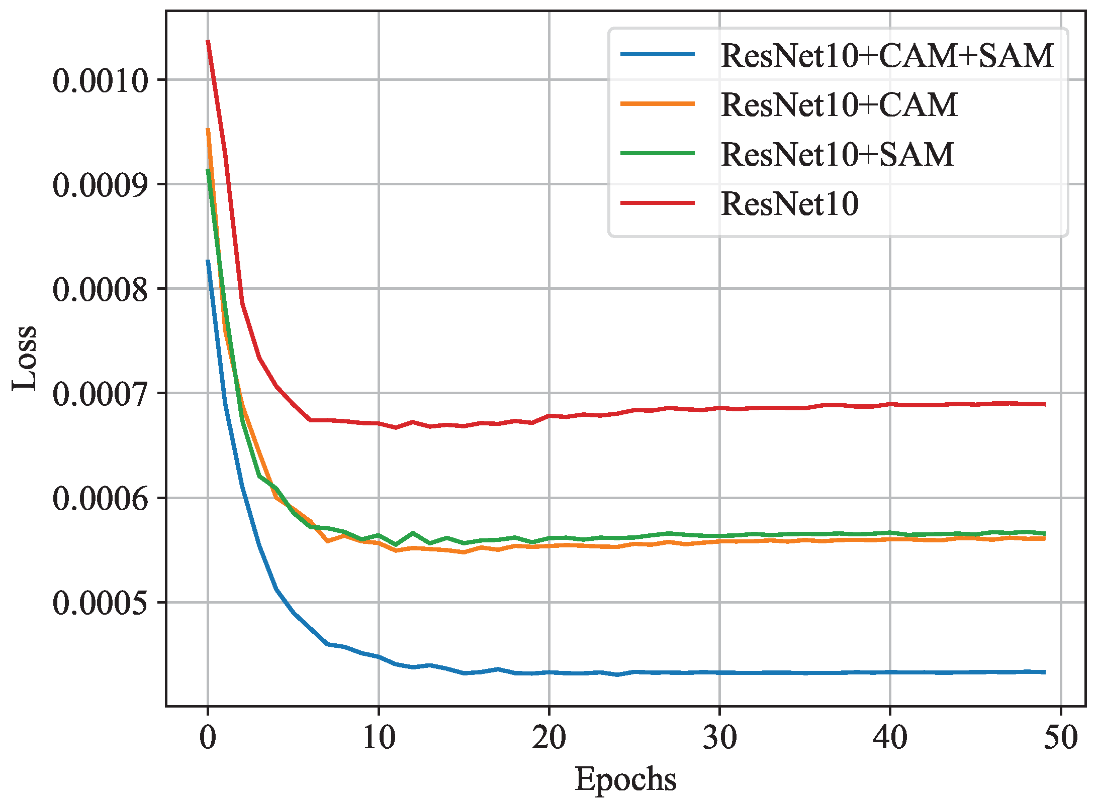
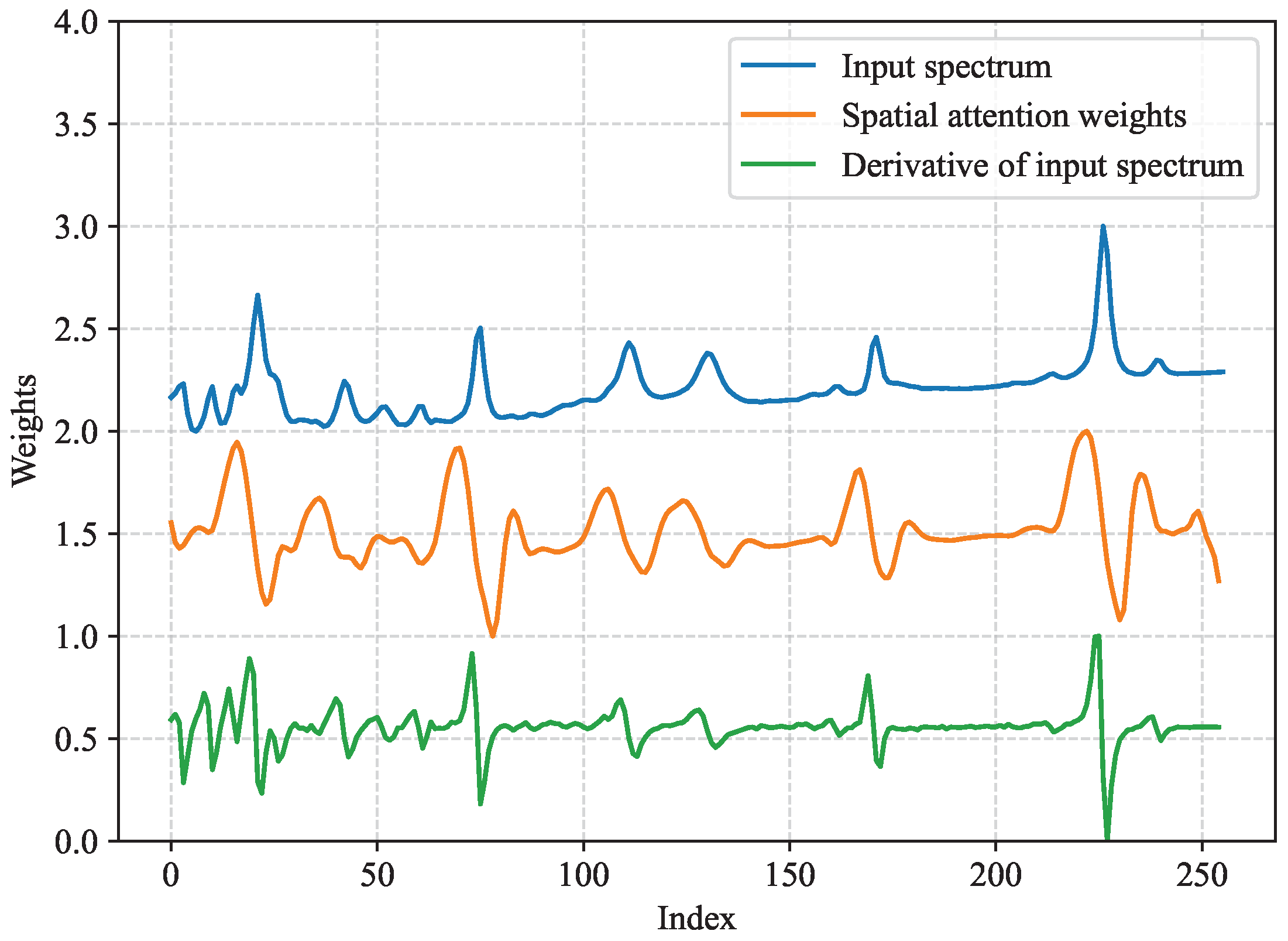
3.5. Effectiveness of Channel and Spatial Attention Modules

To verify the effectiveness of the channel and spatial attention modules, we conducted comparative experiments on four different models used as embedding networks within our Multiplet Network: (1) the baseline model: ResNet10 without any attention mechanisms; (2) the channel attention model: ResNet10 with a channel attention module (CAM); (3) the spatial attention model: ResNet10 with a spatial attention module (SAM); (4) ResNet-CBAM: ResNet10 with both channel and spatial attention modules. In all cases, these models served as the backbone feature extractors for the Multiplet Network, which performed spectral mixture analysis. We trained the models on a dataset containing ${10}^4$ Multiplets, ensuring that all training conditions, including the batch size, learning rate, and optimization strategy, remained consistent across experiments to enable a fair comparison.

Experimental results demonstrated that incorporating attention mechanisms improved classification accuracy and reduced loss, as shown in

Table 2. A performance comparison of different models. The table summarizes the accuracy and loss of the models with and without attention mechanisms. ResNet-CBMA achieved the best performance across both metrics.

Model	Accuracy	Loss
ResNet10	0.77	$6.9\times {10}^{-4}$
ResNet10 + CAM	0.82	$5.6\times {10}^{-4}$
ResNet10 + SAM	0.82	$5.6\times {10}^{-4}$
ResNet10 + CAM + SAM (ResNet-CBMA)	0.87	$4.3\times {10}^{-4}$

. Notably, ResNet-CBMA outperformed other variants, indicating that the combination of channel and spatial attention modules enhanced feature extraction more effectively. Furthermore, as illustrated in Figure 8, the validation loss curves reveal that models with attention mechanisms converged faster and achieved lower final loss values compared to the baseline model. This suggests that attention modules not only enhanced overall model performance but also accelerated convergence and improved generalization capability.

4. Discussion

4.1. Advantages of the Proposed Model

The proposed deep learning-based model demonstrated significant advantages over traditional regression methods in terms of accuracy and the Jaccard Score. This was primarily due to its ability to capture nonlinear relationships and complex spectral feature patterns through multiple layers of nonlinear transformations. Traditional methods, such as Spectral Search [13] and non-negative least squares (NNLS) [14], relied on spectral similarity or distance metrics, which struggled to handle the nonlinear superposition relationships between spectra. Our model’s feature extraction network effectively reduced dimensionality and filtered out noise and non-essential wavelength information while preserving key features that distinguished different components. This capability allowed the model to maintain high precision even in the presence of information overload.

A particularly interesting observation was the remarkable similarity between spatial attention weights and the gradient of the input data. As shown in Figure 9, when the CBAM module was added after the initial convolution layer (conv1) in ResNet, rather than within the residual blocks, the spatial attention weight map of the input data exhibited a high spatial correlation with its gradient map (Pearson correlation coefficient: 0.46; p-value: $1.5\times {10}^{-14}\ll 0.05$), indicating strong consistency. This suggests that the attention mechanism may have allocated weights based on the variation patterns of the input data. Specifically, regions with larger gradients often corresponded to significant changes in the input, and the attention mechanism tended to focus on these areas as they contained more informative features. This phenomenon revealed a potential connection between the attention mechanisms and input data, providing a new perspective on how attention mechanisms function.

4.2. Robustness in Complex Environments

The proposed model exhibited greater robustness to noise and baseline interference compared to traditional methods. While the traditional methods could partially counteract Gaussian noise through averaging, our model further suppressed noise through nonlinear feature enhancement. Additionally, the traditional methods were highly sensitive to uncalibrated linear baseline shifts due to their reliance on baseline correction preprocessing. In contrast, our model automatically removed baseline interference through end-to-end learning, making it more adaptable to instrument drift or sample impurity interference. These characteristics make the proposed model more suitable for rapid retrieval and matching in large-scale spectral libraries, which is critical for accurate multicomponent identification in practical applications.

4.3. Practical Applicability

The strong performance of the proposed model on real-world mixtures highlighted its practical applicability. The Experimental Dataset, which better reflected real-world conditions with lower spectral quality and more realistic component distributions, provided a rigorous test of the model’s robustness. The results demonstrated the model’s ability to accurately identify major components in mixtures, even under increased noise and baseline drift, making it well suited for complex experimental environments. Additionally, the end-to-end optimization process enhanced its capability in mixture composition prediction.

Table 1 presents nine binary and ternary mixtures composed of urea and other common compounds. The model performed well in identifying binary mixtures with high accuracy. However, misidentifications occurred in ternary mixtures. For instance, as shown in Figure 10a, a ternary mixture of S6, S8, and S9 (Figure 10 includes notes indicating the components corresponding to these symbols) was misidentified as containing S3 and S24. Spectral analysis revealed significant overlap between the mixture spectra and those of S3 and S24 at 1047 cm⁻¹, likely leading to false positives. Similarly, Figure 10b shows that S7 was consistently missed in three different mixtures. This may have been due to its weak peak at 940 cm⁻¹, which prevented the model from extracting effective features. The main causes of identification errors in ternary mixtures were likely overlapping spectral features that hindered the differentiation of similar components and weak peak signals that were masked by noise or not effectively extracted.

To enhance model performance, targeted improvements can be implemented. Sensitivity to weak peak signals can be strengthened through specialized training on weak signal data, while detection sensitivity can be improved to better capture weak spectral features. Additionally, introducing sparsity constraints or regularization can help control the number of output components, reducing false positives and improving overall robustness. By adopting these measures, the model’s accuracy in identifying multi-component mixtures, particularly ternary mixtures, is expected to improve significantly.

4.4. Comparison with Existing Methods

Our proposed model distinguishes itself from existing methods in several key aspects. Traditional methods, such as Spectral Search [13] and NNLS [14], rely heavily on spectral similarity metrics and require extensive preprocessing, which can significantly affect recognition outcomes. In contrast, our model leverages deep learning to automatically extract and learn relevant features, reducing the need for manual preprocessing. Compared to DNN-based approaches like DeepCID [18], which requires training a separate CNN model for each compound, our model offers a more efficient and unified framework that captures inter-component relationships. Additionally, unlike DeepRaman [19], which relies on a Pseudo-Siamese neural network and non-negative elastic net, our model integrates attention mechanisms to enhance feature extraction and robustness, eliminating the performance bottleneck associated with the final prediction step. Furthermore, our model’s ability to handle one-shot scenarios, where only a single spectrum per class is available, sets it apart from traditional DNNs that require large-scale mixed spectra for training. This makes our model more practical and adaptable to new datasets without the need for retraining.

5. Conclusions

We proposed a novel model for mixture component identification in Raman spectroscopy, demonstrating superior accuracy and robustness over traditional methods. Specifically, the mixture spectrum and candidate spectra were fed into a feature extractor with shared weights and mapped into a unified feature space using an integrated attention mechanism-based ResNet10 network. In this space, component prediction was performed using least squares, and the model trained the feature extractor by optimizing the loss function, thereby improving identification accuracy. Compared to traditional methods, our deep learning model not only enabled end-to-end feature extraction and component prediction but also captured complex spectral relationships more effectively in the transformed feature space. Furthermore, unlike DNN models that performed direct component identification, our approach first extracted features before predicting mixture components. This allowed our model to adapt to different sizes of candidate spectral libraries and achieve variable-length outputs. On the RRUFF dataset, our model outperformed regression-based approaches, especially in the Jaccard Score, highlighting its effectiveness in spectral analysis. It also maintained a performance advantage as the candidate spectral set expanded and exhibited strong resilience to noise and baseline shifts. On experimentally collected spectra, our model continued to achieve high accuracy despite increased noise and baseline variations, confirming its practical applicability. These results indicate that our approach offers a reliable and adaptable solution for Raman mixture analysis. By effectively capturing complex spectral relationships and adapting to varying conditions, our model stands out as a robust tool for identifying mixture components in Raman spectroscopy.

Moreover, we observed a notable similarity between the spatial attention weights and the derivatives of the input spectral data, indicating a potential link between the attention mechanism and the gradient information of the input. In the future, it would be valuable to explore the explicit integration of gradient information into the design of attention mechanisms. By incorporating a gradient-guided attention module, the model’s ability to capture key features could be further enhanced, potentially boosting its performance in complex tasks.

References

1. Ong, T.T.; Blanch, E.W.; Jones, O.A. Surface Enhanced Raman Spectroscopy in environmental analysis, monitoring and assessment. Sci. Total Environ. 2020, 720, 137601. [Google Scholar] [CrossRef] [PubMed]
2. Sivaprakasam, V.; Hart, M.B. Surface-enhanced Raman spectroscopy for environmental monitoring of aerosols. ACS Omega 2021, 6, 10150–10159. [Google Scholar] [PubMed]
3. Mojica, E.R.; Dai, Z. New Raman spectroscopic methods’ application in forensic science. Talanta Open 2022, 6, 100124. [Google Scholar] [CrossRef]
4. Bērziņš, K.; Boyd, B.J. Surface-Enhanced, Low-Frequency Raman Spectroscopy: A Sensitive Screening Tool for Structural Characterization of Pharmaceuticals. Anal. Chem. 2024, 96, 17100–17108. [Google Scholar] [CrossRef]
5. Petersen, M.; Yu, Z.; Lu, X. Application of Raman spectroscopic methods in food safety: A review. Biosensors 2021, 11, 187. [Google Scholar] [CrossRef]
6. Dong, R.; Wang, J.; Weng, S.; Yuan, H.; Yang, L. Field determination of hazardous chemicals in public security by using a hand-held Raman spectrometer and a deep architecture-search network. Spectrochim. Acta Part A Mol. Biomol. Spectrosc. 2021, 258, 119871. [Google Scholar]
7. Samuel, A.Z.; Mukojima, R.; Horii, S.; Ando, M.; Egashira, S.; Nakashima, T.; Iwatsuki, M.; Takeyama, H. On selecting a suitable spectral matching method for automated analytical applications of Raman spectroscopy. ACS Omega 2021, 6, 2060–2065. [Google Scholar] [CrossRef]
8. Carey, C.; Boucher, T.; Mahadevan, S.; Bartholomew, P.; Dyar, M. Machine learning tools formineral recognition and classification from Raman spectroscopy. J. Raman Spectrosc. 2015, 46, 894–903. [Google Scholar] [CrossRef]
9. Tan, X.; Chen, X.; Song, S. A computational study of spectral matching algorithms for identifying Raman spectra of polycyclic aromatic hydrocarbons. J. Raman Spectrosc. 2017, 48, 113–118. [Google Scholar] [CrossRef]
10. Liu, J.; Osadchy, M.; Ashton, L.; Foster, M.; Solomon, C.J.; Gibson, S.J. Deep convolutional neural networks for Raman spectrum recognition: A unified solution. Analyst 2017, 142, 4067–4074. [Google Scholar] [CrossRef]
11. Hu, J.; Zou, Y.; Sun, B.; Yu, X.; Shang, Z.; Huang, J.; Jin, S.; Liang, P. Raman spectrum classification based on transfer learning by a convolutional neural network: Application to pesticide detection. Spectrochim. Acta Part A Mol. Biomol. Spectrosc. 2022, 265, 120366. [Google Scholar] [CrossRef] [PubMed]
12. Cao, Z.; Pan, X.; Yu, H.; Hua, S.; Wang, D.; Chen, D.Z.; Zhou, M.; Wu, J. A deep learning approach for detecting colorectal cancer via Raman spectra. BME Front. 2022, 2022, 9872028. [Google Scholar] [CrossRef] [PubMed]
13. Vignesh, T.; Shanmukh, S.; Yarra, M.; Botonjic-Sehic, E.; Grassi, J.; Boudries, H.; Dasaratha, S. Estimating probabilistic confidence for mixture components identified using a spectral search algorithm. Appl. Spectrosc. 2012, 66, 334–340. [Google Scholar] [CrossRef]
14. Zhang, Z.M.; Chen, X.Q.; Lu, H.M.; Liang, Y.Z.; Fan, W.; Xu, D.; Zhou, J.; Ye, F.; Yang, Z.Y. Mixture analysis using reverse searching and non-negative least squares. Chemom. Intell. Lab. Syst. 2014, 137, 10–20. [Google Scholar] [CrossRef]
15. Zhao, X.; Liu, C.; Zhao, Z.; Zhu, Q.; Huang, M. Performance Improvement of Handheld Raman Spectrometer for Mixture Components Identification Using Fuzzy Membership and Sparse Non-Negative Least Squares. Appl. Spectrosc. 2022, 76, 548–558. [Google Scholar] [PubMed]
16. Zeng, H.T.; Hou, M.H.; Ni, Y.P.; Fang, Z.; Fan, X.Q.; Lu, H.M.; Zhang, Z.M. Mixture analysis using non-negative elastic net for Raman spectroscopy. J. Chemom. 2020, 34, e3293. [Google Scholar]
17. Van de Sompel, D.; Garai, E.; Zavaleta, C.; Gambhir, S.S. A hybrid least squares and principal component analysis algorithm for Raman spectroscopy. PLoS ONE 2012, 7, e38850. [Google Scholar]
18. Fan, X.; Ming, W.; Zeng, H.; Zhang, Z.; Lu, H. Deep learning-based component identification for the Raman spectra of mixtures. Analyst 2019, 144, 1789–1798. [Google Scholar]
19. Fan, X.; Wang, Y.; Yu, C.; Lv, Y.; Zhang, H.; Yang, Q.; Wen, M.; Lu, H.; Zhang, Z. A universal and accurate method for easily identifying components in Raman spectroscopy based on deep learning. Anal. Chem. 2023, 95, 4863–4870. [Google Scholar]
20. Bromley, J.; Guyon, I.; LeCun, Y.; Säckinger, E.; Shah, R. Signature verification using a “siamese” time delay neural network. Adv. Neural Inf. Process. Syst. 1993, 7, 25. [Google Scholar]
21. Zhao, Z.; Liu, Z.; Ji, M.; Zhao, X.; Zhu, Q.; Huang, M. ConInceDeep: A novel deep learning method for component identification of mixture based on Raman spectroscopy. Chemom. Intell. Lab. Syst. 2023, 234, 104757. [Google Scholar] [CrossRef]
22. Koyun, O.C.; Keser, R.K.; Şahin, S.O.; Bulut, D.; Yorulmaz, M.; Yücesoy, V.; Toreyin, B.U. RamanFormer: A Transformer-Based Quantification Approach for Raman Mixture Components. ACS Omega 2024, 9, 23241–23251. [Google Scholar] [CrossRef] [PubMed]
23. Pan, L.; Pipitsunthonsan, P.; Daengngam, C.; Channumsin, S.; Sreesawet, S.; Chongcheawchamnan, M. Identification of complex mixtures for Raman spectroscopy using a novel scheme based on a new multi-label deep neural network. IEEE Sensors J. 2021, 21, 10834–10843. [Google Scholar] [CrossRef]
24. Liang, J.; Mu, T. Recognition of big data mixed Raman spectra based on deep learning with smartphone as Raman analyzer. Electrophoresis 2020, 41, 1413–1417. [Google Scholar] [CrossRef]
25. Lafuente, B.; Downs, R.T.; Yang, H.; Stone, N.; Armbruster, T.; Danisi, R.M. The power of databases: The RRUFF project. Highlights Mineral. Crystallogr. 2015, 1, 25. [Google Scholar]
26. Hoffer, E.; Ailon, N. Deep metric learning using triplet network. In Proceedings of the Similarity-Based Pattern Recognition: Third International Workshop, SIMBAD 2015, Copenhagen, Denmark, 12–14 October 2015; Proceedings 3. Springer: Berlin/Heidelberg, Germany, 2015; pp. 84–92. [Google Scholar]
27. He, K.; Zhang, X.; Ren, S.; Sun, J. Deep residual learning for image recognition. In Proceedings of the IEEE Conference on Computer Vision and Pattern Recognition, Las Vegas, NV, USA, 26 June–1 July 2016; pp. 770–778. [Google Scholar]
28. LeCun, Y.; Bottou, L.; Bengio, Y.; Haffner, P. Gradient-based learning applied to document recognition. Proc. IEEE 1998, 86, 2278–2324. [Google Scholar] [CrossRef]
29. Woo, S.; Park, J.; Lee, J.Y.; Kweon, I.S. Cbam: Convolutional block attention module. In Proceedings of the European Conference on Computer Vision (ECCV), Munich, Germany, 8–14 September 2018; pp. 3–19. [Google Scholar]
30. Hu, J.; Shen, L.; Sun, G. Squeeze-and-excitation networks. In Proceedings of the IEEE Conference on Computer Vision and Pattern Recognition, Salt Lake City, UT, USA, 18–23 June 2018; pp. 7132–7141. [Google Scholar]
31. Paszke, A.; Gross, S.; Massa, F.; Lerer, A.; Bradbury, J.; Chanan, G.; Killeen, T.; Lin, Z.; Gimelshein, N.; Antiga, L.; et al. Pytorch: An imperative style, high-performance deep learning library. Adv. Neural Inf. Process. Syst. 2019, arXiv:1912.01703. [Google Scholar]
32. Jaccard, P. Étude comparative de la distribution florale dans une portion des Alpes et des Jura. Bull. Soc. Vaudoise Sci. Nat. 1901, 37, 547–579. [Google Scholar]
33. Jaccard, P. The distribution of the flora in the alpine zone. 1. New Phytol. 1912, 11, 37–50. [Google Scholar] [CrossRef]
34. Hamming, R.W. Error detecting and error correcting codes. Bell Syst. Tech. J. 1950, 29, 147–160. [Google Scholar] [CrossRef]
Figure 1. Multiplet Network for mixture Raman spectrum identification.
Photonics 12 00295 g001
Figure 2. The architecture of CBAM-ResNet, where a channel attention module and a spatial attention module are incorporated into each residual block to enhance feature representation.
Photonics 12 00295 g002
Figure 3. Performance comparison of different models in one-shot mixture spectra identification: (a) accuracy, (b) Jaccard Score, (c) Hamming Loss.
Photonics 12 00295 g003
Figure 4. The accuracy of four models at different candidate library sizes. As the candidate library size increased from 5 to 50, the performance of all models declined, but the MN still maintained a superior performance.
Photonics 12 00295 g004
Figure 5. The spectra of potassium chlorate as an example, with Gaussian noise and baseline added: (a) different levels of Gaussian noise added; (b) different levels of baseline shift added.
Photonics 12 00295 g005
Figure 6. The accuracy of four models at different noise and baseline intensities. Gaussian noise with varying intensities (determined by the standard deviation) and linear baselines with varying intensities were introduced to the mixed spectra.
Photonics 12 00295 g006
Figure 7. A comparison of accuracy and the Jaccard Score for four models tested on simulated mixture Raman spectra synthesized from experimental data, with the candidate library size set to 10 and random Gaussian noise and baseline shift added to the mixture spectra.
Photonics 12 00295 g007
Figure 8. Validation loss curves of different models.
Photonics 12 00295 g008
Figure 9. A comparison of the original spectrum, spatial attention weights, and spectral derivative. All curves are scaled and vertically offset for better visualization.
Photonics 12 00295 g009
Figure 10. (a) Displays the spectrum of a mixture composed of S6, S8, and S9, along with its false positive predicted components, S3 and S24. (b) shows that S7 was not identified in any of the three mixture components, and the spectrum of S7 is displayed. (S3 = potassium nitrate; S6 = sodium bicarbonate; S7 = sodium phosphate; S8 = sodium thiosulfate; S9 = oxalic acid; S10 = aluminum hydroxide; S24 = ammonium carbonate).
Photonics 12 00295 g010