Abstract
Compared to traditional mechanical zoom lenses, tunable lenses driven by dielectric elastomers provide clear advantages in zoom range, response speed, and lightweight design. However, these lenses generally employ planar dielectroelastomer actuation, resulting in redundant structures. Additionally, the viscoelastic properties of dielectroelastomer materials often make precise control of focal length difficult. To overcome this issue, this paper introduces a compact, spherical dielectroelastomer-driven tunable lens with a radial size of 20 mm and an effective aperture of 8 mm. A dual-sided actuation structure allows for a 55% adjustment in focal length. Using thermodynamic principles and a spring–viscoelastic rheological model, static and dynamic models of the system have been developed. Experimental results demonstrate that the proposed model accurately predicts the lens’s dynamic response, with a root-mean-square error of less than 0.135, thereby providing a reliable theoretical basis for achieving high-precision focal length control.
1. Introduction
With the widespread use of optical imaging technology in consumer electronics, industrial automation, medical devices, and basic scientific research, traditional systems that rely on mechanical movement of multiple lens groups for zoom and focus have faced challenges in meeting increasing demands for miniaturization, integration, and high performance due to issues like large size, complex structure, and slow response. In this context, tunable lens technology—enabling mechanical-motion-free adjustment through physical field manipulation—has emerged as a new solution for lightweighting and functional integration in optical systems [1]. By directly or indirectly changing lens curvature or refractive index using electrical, thermal, or environmental stimuli, it provides zoom functions without mechanical movement, greatly simplifying system design [2]. Refractive index-modulated lenses (such as liquid crystal lenses) alter the orientation of optical media through external electric fields to produce gradient refractive index distributions [3,4]. Lenses that change curvature mainly utilize liquids or flexible solids. They achieve zoom by directly or indirectly modifying the shape of interfaces or membranes through methods like electro-wetting, shape memory alloy actuation, piezoelectric actuation, or dielectric elastomer actuator (DEA) actuation [5,6].
Dielectric elastomers (DEs) are a type of flexible polymer material, such as silicone rubber and acrylic elastomers, whose operation relies on Maxwell stress generated by electric fields. When voltage is applied, the electrostatic pressure from polarization causes the film to compress in thickness and expand in area, resulting in large strain outputs. Dielectric elastomer-driven tunable lenses (DETLs) offer benefits such as quick response, lightweight design, vibration resistance, low power consumption, and high energy density, demonstrating significant potential in optical systems [7].
Compactness is a key metric for evaluating DETL performance, referring to achieving an extensive focal length range while maintaining a small physical size. Currently, displacement-type zoom DETLs offer a wide zoom range but have a substantial overall length, whereas deformation-type zoom DETLs typically require larger drive areas to achieve increased magnification. Precise control over DETL focal length greatly enhances flexibility and adaptability, and developing mathematical models that accurately describe DETL dynamics is fundamental to achieving such control. However, the dynamic characteristics of liquid-medium DETLs are influenced by multiple factors, including hysteresis, creep, and rate-dependent properties of the dielectroelastomer material, as well as the viscosity of the filling liquid and variations in cavity pressure. These coupled effects significantly increase the difficulty of precisely regulating the lens focal length. Currently, modeling approaches for DEA dynamics can be broadly classified into two types: mechanism-based models and phenomenological models. Mechanism models derive constitutive relationships for stress, electric field, and other variables by treating the DEA as an open thermodynamic system. Starting from the first and second laws of continuum mechanics and irreversible thermodynamics, they construct the Helmholtz free energy (as a function of strain, electric displacement, and internal variables) and incorporate dissipation inequalities. This approach allows for the coupling of multiple physical fields—mechanical, electrical, and thermal—and provides strong physical interpretability. Phenomenological models, however, do not explore underlying mechanisms. Instead, they fit material responses directly by selecting suitable mathematical forms based on macroscopic experimental observations. Their flexible forms and easily identifiable parameters from experiments make them ideal for engineering design and rapid prototyping [8]. Additionally, since fluids are typically treated as incompressible, the hemispherical DEA filled with liquid is constrained by a rigid frame. Modeling requires simultaneously solving two boundary condition sets, volume conservation and surface contour, which further complicates modeling and numerical solutions. Furthermore, current DETL modeling primarily focuses on establishing static models, with limited research dedicated to creating dynamic models that accurately predict DETL’s dynamic behavior [9].
The key points of this work are as follows: First, a spherical dielectric elastic liquid lens driven by a dielectric elastic body was designed and fabricated. The outer electrode of this lens uses a carbon nanotube film. At the same time, the inner side is filled with a glycerol solution containing sodium chloride, which functions as both the lens medium and an electrode. This compact structure offers excellent optical transparency, achieving 84% transmittance across the 380–780 nm wavelength range. By driving one side of the DEA, the focal length can be increased or decreased. Through optimization using the particle swarm algorithm, the focal length variation range reaches 55%. Second, based on thermodynamic theory, hyperelastic material models, and viscoelastic rheological models, nonlinear static and dynamic models for the lens focal length were established, followed by a systematic parameter identification process. Finally, the models were validated through imaging performance and static/dynamic response experiments. Results show that the root mean square error (RMSE) for the static model is 0.0118. For phenomena such as creep, hysteresis, and rate-dependent behavior, the RMSE of model predictions does not exceed 0.135. This validation confirms that the established model effectively describes the static and dynamic behavior of the DETL system, providing a reliable theoretical foundation for model-based, precise focal length control and controller design.
2. Design and Fabrication
The integrated device comprises a lens frame, a dielectric elastomer film, and a glycerol–sodium chloride mixture encapsulated within the cavity, as illustrated schematically in Figure 1a. A carbon nanotube film functions as the electrode on the outer surface of the lens film, combining excellent electrical conductivity with high light transmittance. The glycerol–sodium chloride solution filling the lens cavity is drawn out via a syringe needle, serving both as an optical medium and an electrode, thereby simplifying the device fabrication process. The lens features non-uniform apertures on both sides, with its operating principle illustrated in Figure 1b: Where VS and VL represent the drive voltages applied to the dielectric elastic film on the small aperture side and large aperture side, respectively. In the initial state, VS = VL = 0 V, with the large aperture film, small aperture film, and liquid pressure in equilibrium. When a voltage of magnitude VON is applied to the DEA on the large aperture side (VS = 0 V, VL = VON), the area of the large aperture side film increases while its contraction force on the liquid decreases. This causes the volume of the spherical crown on the large aperture side to expand, reducing its curvature radius. Since the liquid within the cavity is nearly incompressible and total volume is conserved, the volume of the spherical crown on the small aperture side correspondingly decreases, increasing its curvature radius. This ultimately results in an increase in the lens focal length compared to the initial state. Conversely, when voltage is applied to the small aperture side DEA (VS = VON, VL = 0 V), the lens focal length will decrease relative to the initial state. By precisely adjusting the electric field strength on both sides of the DEA, continuous and controllable focal length tuning can be achieved in the zoom direction.
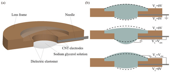
Figure 1.
DETL Schematic Diagram: (a) Structural Schematic; (b) Drive Schematic.
The device fabrication process is shown in Figure 2. First, a carbon nanotube dispersion (Nanjing XFNANO Materials Tech. (Nanjing, China)) was diluted at a 1:200 ratio and filtered under vacuum to create a uniform carbon nanotube electrode film. Next, VHB4905 (3M Company (St. Paul, MN, USA)) was selected as the dielectric elastomer substrate. It was pre-stretched by 250% to enhance driving performance, and the carbon nanotube electrode was transferred to one side of the elastomer film. The prepared DEA was then attached to both sides of the lens frame to form the driving unit. Finally, a glycerol–sodium chloride solution (10 by mass, 0.1) was carefully injected through side holes using a syringe to seal the cavity, ensuring the stable retention of the filling fluid.
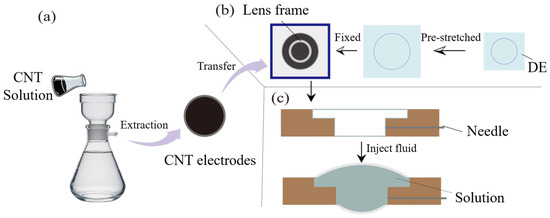
Figure 2.
Flowchart of DETL fabrication process: (a) CNT electrode preparation; (b) DEA preparation; (c) Liquid filling and DETL preparation.
Resistivity was measured using the four-probe method, revealing a resistivity of approximately 2.5 × 10⁶ Ω·m for pure glycerol. Upon addition of NaCl, the resistivity decreased to about 8.9 × 10⁴ Ω·m (measured at 25 °C), meeting the electrode conductivity requirements. Using a refractometer (Abbemat 3200, Anton Paar, Graz, Austria) at a wavelength of 589 nm, the refractive index of the mixed solution was measured as n = 1.455, representing a decrease of approximately 1.2% compared to pure glycerol (n = 1.473). Translated with DeepL.com (free version) The prepared DETL device is shown in Figure 3. It features a distinct double-convex shape and good light transmittance. Measurements using a transmittance meter (CT25, CHN Spec, Hangzhou, China) indicate a transmittance of up to 84% across the 380–780 nm wavelength range, making it suitable for use in optical application equipment.
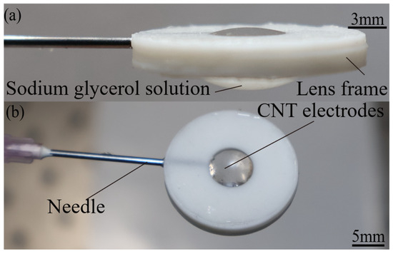
Figure 3.
Physical diagram of DETL: (a) Side view; (b) Top view.
3. Static and Dynamic Models
Due to the influence of material mechanical properties, electro-deformation mechanisms, and viscoelastic effects, the electro-deformation focal length dynamics model of spherical dielectric elasticity-driven tunable lenses exhibits complex nonlinear characteristics. To conduct in-depth research on the focal length variation characteristics of dielectric elasticity-driven tunable lenses under voltage drive, it is necessary to establish systematic static and dynamic models that accurately describe the relationship between the applied voltage u and the focal length f.
First, a force analysis of the spherical DEA based on its lens structure is performed to clarify its mechanical response patterns under applied voltage. Due to the device’s small size, gravitational effects are ignored in this study. Because the force analysis methods for both large-aperture and small-aperture films are identical, only one side of the film is examined, as shown in Figure 4.
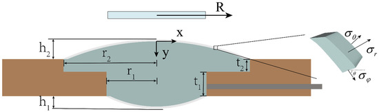
Figure 4.
Schematic diagram of three-axis loading on a lens microelement.
Among these, h1 and h2 represent the crown heights on the small aperture side and large aperture side, respectively; t1 and t2 denote the frame structure thicknesses on the small aperture side and large aperture side of the lens, respectively; r1 and r2 denote the crown radii on the small aperture side and large aperture side, respectively; is the radial strain of the film; is the angle between the tangent direction at point R and the horizontal direction under deformation. Initially, the film thickness is T, and R can describe the position of a microelement on the film. After undergoing isotropic pre-stretching by a factor of , the radius expands to R0. After injecting a liquid volume V0, the film takes on a spherical cap shape. A coordinate system is set with the vertex of the spherical cap as the origin, and the internal cavity pressure p0 is assumed to be evenly distributed. From geometric relationships, we obtain:
By solving dx and dy, the contour curve of the thin film can be obtained, where the stretch ratio in the latitude direction is:
The force balance between the film in the y-direction and the latitude direction can be expressed as follows [10,11]:
Among them, is the thickness of the film after deformation, , is the stress generated in the film in the radial direction, and p is the internal pressure of the cavity. Assuming that the material is incompressible, then . Equations (1)–(3) can be obtained from Equations (4) and (5):
Combining the hyperelastic constitutive model of dielectric elastomers, the stresses and in the radial and transverse directions of the film can be expressed by the free energy density Ws and the constitutive parameters and of the material. Ignoring the stress across the thickness of the film, the relationship between the stress of the dielectric elastomer and the constitutive parameters is [12]:
Among them, ε is the dielectric constant of the dielectric elastic body, , and u is the magnitude of the applied drive voltage. In this paper, the Gent model is selected as the deformation free energy function of the dielectric elastic body:
Among these, μ represents the shear modulus of the elastomer, while Jlim denotes a dimensionless material constant associated with ultimate tensile strength. Solving the differential equations using combinations (1)–(3) and (6)–(9) yields the profiles of the spherical crowns on both sides of the lens under different voltages.
Although the static model effectively describes the hyperelastic behavior and electromechanical coupling effects of dielectroelastomer-driven tunable lenses, both experimental data and literature evidence show that dielectroelastomer materials also display significant hysteresis and creep characteristics. This viscoelastic behavior significantly affects the accuracy and long-term stability of the lenses’ dynamic response [13]. To systematically incorporate these viscoelastic effects into the model, this paper introduces a generalized Maxwell model. Specifically, the total stress in the dielectric elastomer is decomposed into mechanical elastic stress and viscoelastic stress , as illustrated in Figure 5.
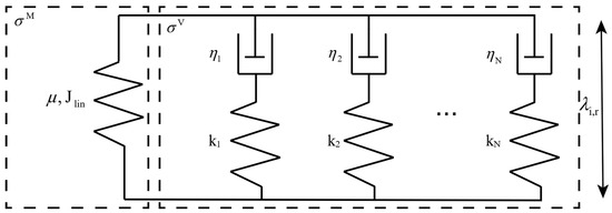
Figure 5.
Schematic Diagram of the Dielectric Elastomer Dynamic Model.
Among these, is described by the Gent hyperelastic constitutive relationship, while is given by the superposition of several spring-damper elements within the generalized Maxwell model. Its dynamic equations are characterized by the strain rate and the spring stiffness and damping coefficients of each branch [14,15]:
In this model, i = , , j = 1,…,N, where N denotes the number of parallel spring–viscoelastic units, represents the internal viscoelastic strain, kj and are the model parameters representing the stiffness coefficient and damping coefficient of each unit, respectively, and is the electric drive strain ratio. This decomposition ensures that the model maintains physical consistency with the hyperelastic static response while capturing hysteresis, creep, and frequency-dependent dynamic characteristics through a set of identifiable parameters. This provides a reliable theoretical foundation for accurately simulating the dynamic behavior of metalenses and designing controllers. By combining the viscoelastic stress with the hyperelastic mechanical stress, a comprehensive dynamic stress expression is formed, leading to the viscoelastic dynamic model of the dielectric elastic body:
Based on the lens configuration, it is evident that at the origin of the coordinate system, x = y = = 0, and the edge of the frame at x = r2. Since the fluid can be considered incompressible, the volume of liquid inside the lens stays constant:
where Vsmall, Vlarge, and Vframe represent the volumes of the small-aperture-side spherical crown, the large-aperture-side spherical crown, and the lens frame, respectively. Among these, t1 and t2 represent the frame structure thicknesses on the large aperture side and small aperture side of the lens, respectively. Under the specified boundary conditions, first set the radial strain ratio estimate at the coordinate origin and the initial liquid pressure estimate p0_guess. Using the established model and applying the target-hitting method for iterative solutions, the actual radial strain ratio of the thin film and the proper pressure distribution of the liquid are ultimately determined, thereby defining the final contour of the lens. Based on the structural parameters of the lens, the curvature radii of the two spherical halves were calculated using the formula:
Here, h and r denote the radius and thickness of the spherical cap, respectively. Subsequently, its focal length can be calculated using the formula for thick lenses [16]:
Here, n denotes the refractive index of the injected liquid, while R1 and R2 represent the radii of curvature for the spherical caps on the small-aperture side and large-aperture side, respectively.
4. Result and Discussion
4.1. Structural Optimization
Based on the established static model of the focal length, a particle swarm optimization algorithm is used to optimize three parameters—aperture radius on both sides of the lens and filling liquid volume—with the maximum focal length variation range as the objective function. The iterative update formula is as follows:
Among these, and represent the predicted value and increment of the jth component of the ith particle at the kth iteration, respectively. w denotes the inertia weight, while c1 and c2 denote the individual and population learning factors, respectively. r1 and r2 are random numbers distributed within [0,1], and pbesti,j and gbestj denote the individual and global optimal values, respectively. Based on the above iterative strategy, particle positions and velocities are updated to approach the optimal solution progressively.
During optimization, the pre-stretch ratio was set to 2.5, with material parameters and Jlim set to 14.78 kPa and 244, respectively. The frame structure thicknesses t1 and t2 on the small-aperture and large-aperture sides of the lens were 2 mm and 1 mm, respectively. The iterative solution yielded the following optimal design parameters: small aperture side radius r1 = 4.03 mm, large aperture side radius r2 = 7.50 mm, and filling liquid volume V0 = 0.57 mL.
4.2. Experimental Platform
To thoroughly and precisely verify the performance of the proposed DETL, an experimental platform was built as shown in Figure 6a. The platform includes two high-voltage amplifiers, a control module, a laser displacement sensor, and the DETL under test. The drive signal output from the control module regulates the output voltage of the high-voltage amplifier, thereby altering the electric field distribution across the DEA and adjusting the lens focal length.
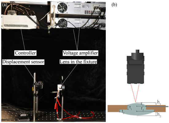
Figure 6.
Diagram of the experimental platform and measurement principle: (a) Physical diagram of the experimental platform; (b) Measurement schematic.
The specific measurement method is shown in Figure 6b, where a laser displacement sensor is used to monitor in real time the height difference h1 between the top and bottom of the spherical crown on the small aperture side of the lens. The structural parameters t1, t2, r1, and r2 of the lens frame are known constants. Combining this with Equation (12), the lens frame volume Vframe is also a constant. Based on the measurement data, the real-time volume Vsmall of the small-aperture-side spherical crown can be calculated. Since the filling liquid is approximately incompressible, the total cavity volume V0 remains constant. The volume of the large-aperture-side spherical crown can be derived from Equation (12). Furthermore, the height h2 of the large-aperture-side spherical crown can be obtained from Equation (12). Finally, using Equation (13) to calculate the curvature radii of both spherical halves, and combining this with the thick lens focal length formula in Equation (14), the real-time focal length f of the lens can be obtained [17].
4.3. Performance Testing
To thoroughly assess the dynamic response and zoom capability of the proposed DETL, this study performed tests for imaging performance, zoom range, response time, and power consumption. Since the designed device can operate stably under a 2 kV DC drive, the test voltage range was set to 0–2 kV.
To verify the device’s suitability in imaging systems, the DETL was placed within the optical path, and a camera captured the changes in images of the same target under different drive voltages. The resulting images are shown in Figure 7a. When the voltage on the small aperture side was zero and the voltage on the large aperture side was gradually increased, the target characters “DE” progressively enlarged on the camera screen. Conversely, when the voltage on the large aperture side was set to zero and the voltage on the small aperture side was gradually increased, the character image shrank. To characterize the resolution of the tunable lens, imaging tests were conducted with the USAF Resolution Target (USAF 1951) positioned in front of the lens. Voltages of 0.5 kV, 1.0 kV, 1.5 kV, and 2.0 kV were applied to the DEA on both the large-aperture side and the small-aperture side. A CCD camera was used in conjunction with the tunable lens to record the imaging results. The experimental results are shown in Figure 7b: Under optimal imaging conditions, the lens achieved a minimum resolution of the first element in the fifth group, corresponding to 32 lp/mm. The imaging experiments demonstrate that the DETL exhibits excellent focal length adjustment capability and imaging clarity, though certain aberrations remain. This may stem from distortion caused by non-uniform stretching of the film and chromatic aberration resulting from refractive index variations across different wavelengths in the liquid lens material. Subsequent work will involve precise measurement of these aberrations and implementing strategies such as real-time correction through computational imaging and digital post-processing algorithms, optimizing the film pre-stretching process and electrode distribution to enhance surface accuracy, and introducing compensatory optical elements to improve imaging quality [18,19].
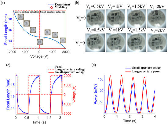
Figure 7.
Zoom Performance Testing: (a) Zoom Effect and Model Validation; (b) Resolution Testing; (c) Response Time Testing; (d) Power Testing.
During zoom range testing, a step drive voltage was applied to the large and small aperture DEAs, with the voltage increasing from 0 V to 2 kV in 400 V increments of 2 s. The experimentally measured focal lengths at different drive voltages (red dots) were compared with the simulation results from the established model (blue line), as shown in Figure 7a. The dashed red box and solid red box represent the experimental and simulation results for the large-aperture side and small-aperture side drive, respectively. Test results indicate that the lens exhibits a focal length variation of up to 55% (12.66 mm–19.66 mm) and a refractive power variation of up to 28 D. The root mean square error (RMSE) of the static model’s prediction for the focal length-voltage relationship is 0.0118, demonstrating high accuracy within the static range.
In response time measurements, a square wave drive signal with a frequency of 1 Hz, a duty cycle of 50%, and an amplitude of 2 kV was applied to the DEA on both the large-aperture and small-aperture sides. The phase difference between the two sides was set to 500 ms. The dynamic response, as shown in Figure 7c, typically comprises two stages: a rapid rise and a slow creep. The rapid stage represents the transient electrodynamic deformation of the dielectric elastomer film under voltage, primarily driven by the elastic stress term in Equation (8). The slow stage is mainly attributed to the viscoelastic behavior of the material, whose contribution is reflected in the viscoelastic stress terms of Equations (10) and (11). The rise time (from minimum to maximum focal length) was calculated using the 90% criterion of the change in amplitude; similarly, the fall time (from maximum to minimum focal length) was also calculated using the 90% criterion [20]. Experimental results indicate that the rise time of this device is approximately 280 ms, and the fall time is approximately 180 ms.
In the power consumption test, a cosine voltage with an amplitude of 1 kV, a bias of 1 kV, and a frequency of 1 Hz was applied to the large-aperture and small-aperture DEAs. The drive current was measured through the current monitoring interface of the high-voltage source, and the real-time power was calculated accordingly. The power variation over time is shown in Figure 7d. The average powers of the large-aperture and small-aperture DEAs were 64.215 mW and 49.88 mW, respectively, with a peak power of 166.84 mW [21].
4.4. Dynamic Model Validation
To accurately determine the parameters of the DETL kinetic model, a range of drive voltages with various amplitudes and frequencies was applied to both the large and small aperture sides during the experiment. The specific signal forms included as follows [22]:
In this context, i = 1, 2, 3, 4, 5, j = 1, 2, …, 10, Ai,j represents the signal amplitude, ti,j denotes the starting time of the time interval, fi = 0.1i signifies the signal frequency, and T indicates the half-period length. By simultaneously acquiring the drive voltage and laser displacement sensor output under the aforementioned conditions, parameter identification is conducted on the established DETL dynamic model. The parameters to be identified include the elasticity and viscosity-related coefficients: k1, k2, k3, k4, , , , and . Based on the collected training data, systematic parameter identification was carried out using least-squares fitting and time-series optimization techniques. The results of the parameter identification are shown in Table 1.

Table 1.
Identification table for parameters on the large-aperture and small-aperture sides.
After completing the parameter identification, validation experiments were conducted using drive signals at various frequencies. The validation data included 25-s drive signals at 0.2, 0.4, 0.6, 0.8, and 1.0 Hz, each with amplitude variations. To quantitatively assess the model’s prediction accuracy, the root mean square error erms and maximum tracking error em are introduced as performance metrics:
fe and fm represent the experimentally measured focal length and the model-predicted focal length, respectively, where N denotes the total number of sampling points. The experimental results are shown in Table 1 and Figure 8. The findings are summarized in Table 2 and Figure 8. The results indicate that under small-aperture side-drive conditions, the model-predicted root mean square error does not exceed 0.1350; under large-aperture side-drive conditions, the root mean square error does not exceed 0.0974.
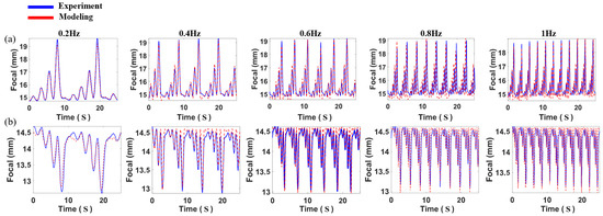
Figure 8.
Comparison of model and experimental results under drive signals with different frequencies and amplitude values: (a) Large aperture side drive; (b) Small aperture side drive.
Table 2.
erms and em driven by large aperture/small aperture at different frequencies.
Although the established dynamic model can predict the trend of DETL’s dynamic response to some extent, prediction errors still occur. These errors primarily arise from the following factors: First, the model’s force analysis assumptions overlook fluid inertia effects and gravitational influences, which become significant at higher frequencies, leading to deviations in phase and amplitude predictions. Second, during parameter identification, although the generalized Maxwell model parameters were derived from dynamic experimental data at various frequencies and amplitudes, they may not fully represent the material’s viscoelastic behavior across all frequency ranges. Future work will further enhance the model by incorporating equations for gravity and fluid dynamics to improve its accuracy.
5. Conclusions
This paper introduces and validates a spherical dielectroelastically driven liquid lens along with its modeling method. First, a compact spherical DE-driven liquid lens was constructed. Its outer surface utilizes a carbon nanotube film as a transparent electrode. At the same time, the interior is filled with a glycerol–sodium chloride solution, serving as both the optical medium and the electrode, thereby simplifying device fabrication. By actuating the DEAs on opposite sides, reversible adjustments of the focal length can be achieved. Structural optimization using particle swarm optimization yielded a measured zoom range of 55%. Second, a nonlinear static–dynamic coupled model for the lens’s focal length was developed based on irreversible thermodynamics, hyperelastic constitutive models, and generalized Maxwell rheology. Experimental data were systematically used to determine model parameters, ensuring the model remains physically consistent with static hyperelastic responses while accurately describing the viscoelastic behavior of the material. Validation was performed through imaging performance tests and static/dynamic response experiments. The root-mean-square error for the static model was 0.0118, while the errors for dynamic behaviors, such as creep, hysteresis, and rate dependence, did not exceed 0.135. Results show that the model effectively captures both static and dynamic behaviors of the DETL system. This work advances device design and dynamic modeling of DETL. The model provides a solid theoretical basis for developing precise focal length control strategies and controllers. It also offers a technical solution for applying DE-driven adjustable lenses in portable imaging, adaptive optics, and other compact zoom applications. However, the accuracy of the lens’s aberration and dynamic models still needs improvement. In the future, the model will be further refined by integrating gravity and fluid dynamics models. Active control of focal length and aberration will be implemented to further improve the performance of the DETL.
Author Contributions
Conceptualisation, Z.H. and H.H.; methodology, Z.H., Z.L. and H.H.; investigation, Z.H., M.Z., Z.G. and J.L.; writing—original draft preparation, Z.H., M.Z. and Z.G.; software, Z.H. and J.L.; writing—review and editing, M.Z. and Z.G.; visualisation, Z.H. and Z.L.; supervision, H.H.; project administration, M.Z. and Z.G.; funding acquisition, H.H. and M.Z. All authors have read and agreed to the published version of the manuscript.
Funding
This research received no external funding.
Institutional Review Board Statement
Not applicable.
Informed Consent Statement
Not applicable.
Data Availability Statement
The raw data supporting the conclusions of this article will be made available by the authors on request.
Conflicts of Interest
The authors declare no conflicts of interest.
References
- Land, M.F. The Evolution of Lenses. Ophthalmic Physiol. Opt. 2012, 32, 449–460. [Google Scholar] [CrossRef]
- Ren, H.; Wu, S.-T. Introduction to Adaptive Lenses-2012-Ren; Wiley: Hoboken, NJ, USA, 2012; ISBN 978-1-118-01899-6. [Google Scholar]
- Tian, L.-L.; Hu, W.; Zhou, H.-Z.; Yu, L.; Li, L.; Li, L. SRGAN Algorithm-Assisted Electrically Controllable Zoom System Based on Pancharatnam-Berry Liquid Crystal Lens for VR/AR Display. ACS Photonics 2024, 11, 2787–2796. [Google Scholar] [CrossRef]
- Yu, L.; Jiang, X.-K.; Hu, W.; Guo, Z.; Li, Y.; Zeng, Y.-M.; Tian, L.-L. Large Aperture Liquid Crystal Lens Array Based on Integrated Composite Electrodes for 2D/3D Switchable Displays. Displays 2024, 81, 102612. [Google Scholar] [CrossRef]
- Liu, C.; Zheng, Y.; Yuan, R.; Jiang, Z.; Xu, J.; Zhao, Y.; Wang, X.; Li, X.; Xing, Y.; Wang, Q. Tunable Liquid Lenses: Emerging Technologies and Future Perspectives. Laser Photonics Rev. 2023, 17, 2300274. [Google Scholar] [CrossRef]
- Chen, L.; Ghilardi, M.; Busfield, J.J.C.; Carpi, F. Electrically Tunable Lenses: A Review. Front. Robot. AI 2021, 8, 678046. [Google Scholar] [CrossRef] [PubMed]
- Chen, Y.; Zhao, H.; Mao, J.; Chirarattananon, P.; Helbling, E.F.; Hyun, N.P.; Clarke, D.R.; Wood, R.J. Controlled Flight of a Microrobot Powered by Soft Artificial Muscles. Nature 2019, 575, 324–329. [Google Scholar] [CrossRef] [PubMed]
- Li, Z.; Chen, G.; Xu, H.; Chen, X.; Shan, J.; Zhang, X. A review of modeling and control methods for dielectric elastomer actuator systems (Chinese). Control. Decis. 2023, 38, 2283–2300. [Google Scholar] [CrossRef]
- Hu, Z.; Zhang, M.; Gan, Z.; Lv, J.; Lin, Z.; Hong, H. Tuneable Lenses Driven by Dielectric Elastomers: Principles, Structures, Applications, and Challenges. Appl. Sci. 2025, 15, 6926. [Google Scholar] [CrossRef]
- Li, T.; Keplinger, C.; Baumgartner, R.; Bauer, S.; Yang, W.; Suo, Z. Giant Voltage-Induced Deformation in Dielectric Elastomers near the Verge of Snap-through Instability. J. Mech. Phys. Solids 2013, 61, 611–628. [Google Scholar] [CrossRef]
- Wang, F.; Yuan, C.; Lu, T.; Wang, T.J. Anomalous Bulging Behaviors of a Dielectric Elastomer Balloon under Internal Pressure and Electric Actuation. J. Mech. Phys. Solids 2017, 102, 1–16. [Google Scholar] [CrossRef]
- He, T.; Cui, L.; Chen, C.; Suo, Z. Nonlinear Deformation Analysis of a Dielectric Elastomer Membrane–Spring System. Smart Mater. Struct. 2010, 19, 85017. [Google Scholar] [CrossRef]
- Gu, G.-Y.; Gupta, U.; Zhu, J.; Zhu, L.-M.; Zhu, X. Modeling of Viscoelastic Electromechanical Behavior in a Soft Dielectric Elastomer Actuator. IEEE Trans. Robot. 2017, 33, 1263–1271. [Google Scholar] [CrossRef]
- Rizzello, G.; Naso, D.; York, A.; Seelecke, S. Modeling, Identification, and Control of a Dielectric Electro-Active Polymer Positioning System. IEEE Trans. Contr. Syst. Technol. 2015, 23, 632–643. [Google Scholar] [CrossRef]
- Li, Y.; Oh, I.; Chen, J.; Zhang, H.; Hu, Y. Nonlinear Dynamic Analysis and Active Control of Visco-Hyperelastic Dielectric Elastomer Membrane. Int. J. Solids Struct. 2018, 152–153, 28–38. [Google Scholar] [CrossRef]
- Hecht, E. Optics, 4th ed.; International, Ed.; Addison-Wesley: Reading, MA, USA, 2002; ISBN 978-0-8053-8566-3. [Google Scholar]
- Pieroni, M.; Lagomarsini, C.; De Rossi, D.; Carpi, F. Electrically Tunable Soft Solid Lens Inspired by Reptile and Bird Accommodation. Bioinspir. Biomim. 2016, 11, 65003. [Google Scholar] [CrossRef] [PubMed]
- Liu, Z. Research on Image Quality Enhancement Method for Compact Liquid-Zoom Vision Systems Based on Computational Imaging Technology. Opt. Laser Technol. 2025, 192, 113692. [Google Scholar] [CrossRef]
- Zhan, T.; Zou, J.; Xiong, J.; Liu, X.; Chen, H.; Yang, J.; Liu, S.; Dong, Y.; Wu, S.-T. Practical Chromatic Aberration Correction in Virtual Reality Displays Enabled by Cost-effective Ultra-broadband Liquid Crystal Polymer Lenses. Adv. Opt. Mater. 2020, 8, 1901360. [Google Scholar] [CrossRef]
- Lv, J.; Hong, H.; Gan, Z.; Zhang, M.; Liu, Z.; Hu, Z. Dielectric Elastomer-Driven Liquid Prism Enabling Two-Dimensional Beam Control. Opt. Express 2024, 32, 21517. [Google Scholar] [CrossRef] [PubMed]
- Du, B.; Tang, C.; Jiang, S.; Wang, Y.; Liu, X.-J.; Zhao, H. High-speed Rotary Motor for Multidomain Operations Driven by Resonant Dielectric Elastomer Actuators. Adv. Intell. Syst. 2023, 5, 2300243. [Google Scholar] [CrossRef]
- Huang, P.; Ye, W.; Wang, Y. Dynamic Modeling of Dielectric Elastomer Actuator with Conical Shape. PLoS ONE 2020, 15, e0235229. [Google Scholar] [CrossRef] [PubMed]


Disclaimer/Publisher’s Note: The statements, opinions and data contained in all publications are solely those of the individual author(s) and contributor(s) and not of MDPI and/or the editor(s). MDPI and/or the editor(s) disclaim responsibility for any injury to people or property resulting from any ideas, methods, instructions or products referred to in the content. |
© 2025 by the authors. Licensee MDPI, Basel, Switzerland. This article is an open access article distributed under the terms and conditions of the Creative Commons Attribution (CC BY) license (https://creativecommons.org/licenses/by/4.0/).