Article

High-Performance 3D Point Cloud Image Distortion Calibration Filter Based on Decision Tree

The School of Artificial Intelligence, Hubei University, Wuhan 430062, China
Photonics 2025, 12(10), 960; https://doi.org/10.3390/photonics12100960 (registering DOI)
Submission received: 18 August 2025 / Revised: 15 September 2025 / Accepted: 15 September 2025 / Published: 28 September 2025

Abstract

Structured Light LiDAR is susceptible to lens scattering and temperature fluctuations, resulting in some level of distortion in the captured point cloud image. To address this problem, this paper proposes a high-performance 3D point cloud Least Mean Square filter based on Decision Tree, which is called the D−LMS filter for short. The D−LMS filter is an adaptive filtering compensation algorithm based on decision tree, which can effectively distinguish the signal region from the distorted region, thus optimizing the distortion of the point cloud image and improving the accuracy of the point cloud image. The experimental results clearly demonstrate that our proposed D−LMS filtering algorithm significantly improves accuracy by optimizing distorted areas. Compared with the 3D point cloud least mean square filter based on SVM, the accuracy of the proposed D−LMS filtering algorithm is improved from 86.17% to 92.38%, the training time is reduced by 1317 times and the testing time is reduced by 1208 times.

1. Introduction

Structural Light LiDAR faces multiple challenges when capturing point cloud images, with lens scattering and temperature variations standing out prominently among the adverse factors. These factors often result in imperfect data acquisition by the LiDAR system [1,2,3].
Specifically, lens scattering causes the laser beam to scatter during the transmission process, which will affect the accuracy results of structural light lidar in measuring the distance and position of the target object. In addition, temperature variations can cause fluctuations in the performance of internal optical components of structural light lidar, further affecting the stability of data collection. The combination of these factors leads to significant distortion in the final point cloud image, particularly around the edges. This distortion not only reduces the accuracy and reliability of the image, but also poses considerable challenges for subsequent data analysis and processing [4,5]. In addition, limited statistical frame data and atmospheric sheltering can also lead to significant backscattering, which substantially limits the depth imaging capability of LiDAR systems in strong scattering environments [6,7,8,9,10]. Therefore, effectively addressing these challenges is crucial for improving the performance of structured light lidar.
To address these challenges, researchers have designed various point cloud distortion correction methods. In the process of calibrating the data collected by Kinect sensor [11,12,13,14,15], Kourosh Khoshelham established a mathematical model of depth measurement, and analyzed the systematic error and random error [16]. However, traditional error models assume a homogeneous noise distribution, whereas the noise in structured-light LiDAR follows a Poisson-Gaussian hybrid model with spatially varying parameters [17,18,19], thereby invalidating classical calibration approaches in edge regions. As the distance between the target and the sensor increases, the measurement error will also increase. Among them, the correction of systematic error is the prerequisite for aligning depth data and color data, while random error is crucial in further processing depth data [20]. In order to reduce the negative impact of image distortion, Hong-Xiang Chen proposed a distortion-tolerant omnidirectional depth estimation algorithm using a dual-cubemap [21]. By introducing a distortion-aware module and a plug-and-play spherical perception weight matrix, the algorithm addresses the issue of uneven distribution of regions projected from a sphere, helping to reduce the supervision deviation caused by distortion. In solving geometric distortion problems such as rotation, scaling, and translation, Navnath S. Narawade proposed a method for correcting geometric distortion in images based on pixel and size [22]. This method effectively enhances the ability to correct geometric distortion by combining spy pixel technology and size geometric distortion correction module. In the scanning process of precision instruments, hysteresis and thermal drift can cause the actual position of the scanning points to deviate from the expected position, thereby significantly affecting imaging results [23,24]. To address this issue, Yinan Wu designed a hysteresis compensation algorithm based on B-spline curve fitting to correct the distortion region. In addition, the team proposed a novel off-line drift correction algorithm based on cross diagonal scanning to rectify the captured distorted images [24].
When depth images are compressed, severe boundary distortion may occur. Linear filtering can result in excessive smoothing of the edges in depth images, while non-linear filtering can preserve edge features through non-linear operations. For example, De Silva proposed a bilateral filter with adaptive filtering parameters, which can preserve the edge features by non-linear combination of adjacent pixel values through spatial distance and pixel similarity [25,26]. Additionally, Shujie Liu proposed a trilateral filtering method, which takes into account the spatial correlation and luminance similarity of the depth image and the color image [27]. Furthermore, Kwan-Jung Oh put forward a depth boundary reconstruction filter, which can be used as an in-loop filter for depth video coding [28]. Xuyuan Xu presented a low-complexity adaptive deep truncation filter that can significantly reduce compression artifacts in depth images [29]. However, a drawback of this method is the distortion and deformation it may cause in certain uneven regions, such as slope distortion and surface deformation. Considering that the previous work only utilizing spatial correlation and statistic property of local windows [30], Lijun Zhao proposed a global approach to address the problem of generating high-resolution range images by Markov Random Field (MRF) model, which can be used to eliminate artifacts in discontinuous regions of distorted depth images [31].
The above distortion calibration algorithms are overly complex, and the majority of them focus on two-dimensional image distortion calibration. To overcome these challenges, this paper proposes a high-performance 3D point cloud least mean square filter based on decision tree, which is called D−LMS filter for short. Firstly, the decision tree model can be used to extract features from the point cloud image, complete the segmentation of signal region and distortion region, and detect the positions of all points in the distortion region. Secondly, the adaptive least mean square filter is implemented to correct the points in the distorted region, thereby optimizing the distortion of the point cloud image and enhancing its accuracy.
To sum up, the D−LMS filter combines the classification and prediction ability of decision tree and the optimization performance of the adaptive least mean square filter, which makes it more accurate and robust when dealing with complex non-linear signals. In addition, the D−LMS filter has strong adaptive capabilities, and can automatically adjust the filtering parameters according to the changes in signals, resulting in even better filtering performance.
The rest of this paper is organized as follows: Section 2 lays out the principle of the proposed high-performance 3D point cloud Least Mean Square filter based on Decision Tree. Section 3 analyzes the training time and testing time of the D−LMS filtering model. Section 4 describes the performance of point cloud image distortion calibration in the experiment. Finally, conclusions are drawn.

2. High-Performance 3D Point Cloud Least Mean Square Filter Based on Decision Tree

The logic of the proposed high-performance 3D point cloud least mean square filter based on decision tree is outlined in Figure 1, which encompasses two primary phases: the training phase and the testing phase.
In the training phase, the proposed D−LMS algorithm utilizes a decision tree model to learn and identify the distorted regions in 3D point cloud images. The ultimate goal of this learning process is to divide the point cloud image into signal region and distortion region, so as to extract the corresponding point data. In the testing phase, an adaptive least mean squares (LMS) filter is used to refine the points within the distorted region. This process aims to reduce distortion present in the point cloud image, thereby significantly enhancing its overall accuracy and fidelity.

2.1. Training Phase

In the training phase, this article introduces a decision tree model to complete the training process of point cloud data. The decision tree is a supervised learning algorithm used for classification and regression tasks. It makes decisions based on a tree structure and has a very fast classification speed [32].
The algorithm primarily consists of three key steps: feature selection, where important variables are identified; decision tree generation, where the structure of tree is constructed based on these variables; and decision tree pruning, where the tree is optimized for better performance and simpler interpretation. These steps work together to create a powerful tool that can help solve complex problems in various fields. In our background, it is used to classify points in 3D point cloud into signal regions or distorted regions.
Assuming that the training dataset contains m point cloud images, with each image having p points, the training dataset D can be represented as
D = x 1 , y 1 , x 2 , y 2 , , x M , y M
where x i (i = 1, 2…, M) is a column vector containing three-dimensional coordinates and intensity values, y i is the corresponding signal label or distortion label, and M = m p is the number of points included in the training dataset D .
The attribute set A defined in this paper includes the following five core features:
(1)
Point Density: ρ p i = N π r 2 . It reflects the richness of data in local regions, where distorted areas typically exhibit abnormal density due to sensor errors.
(2)
The normal vector: θ p i = 1 N j = 1 N c o s n i ,   n j . The normal vectors in signal regions tend to be consistent, whereas those in distorted regions tend to be scattered.
(3)
Neighborhood Variance: σ 2 p i = 1 N j = 1 N z j z ¯ 2 . The variance in distorted regions is significantly higher than that in signal regions due to noise interference.
(4)
Local Curvature: κ ρ i = λ 3 λ 1 + λ 2 + λ 3 . The curvature in signal regions tends to be close to zero, whereas regions along edges or areas with distortion exhibit higher curvature values.
(5)
Intensity Gradient: I p i = I x 2 + I y 2 + I z 2 . Abnormal fluctuations in reflection intensity may occur in distortion areas due to sensor errors.
Algorithm 1 lays out the main principle of the decision tree model. Initially, the information gain of all features is calculated from the root node, and the feature with the largest information gain is selected as the feature of the node. Then, a child node is established according to the feature result, and the above method is called recursively for the child node. Finally, a decision tree is constructed until all features are selected. The goal is to construct a decision tree model T according to the given training dataset D , so that it can correctly classify the target point cloud into signal point cloud and distorted point cloud, and the loss function needs to be minimized in the learning process.
To prevent the degradation of generalization performance caused by overfitting to noisy data during the training process of the decision tree model, this paper adopts a strategy that combines pre-pruning and post-pruning to optimize the tree structure.
During the growth process of the decision tree, pre-pruning terminates branch expansion in advance based on the following criteria. The purpose is to limit the depth of the tree to prevent over-fitting, while preserving the key features (such as high curvature and high variance) in the distorted regions of the point cloud.
(1)
Minimum sample size threshold: the splitting is stopped when the number of samples contained in the current node is less than τ m i n .
(2)
Information gain threshold: If the information gain after splitting is less than τ g a i n , the split is rejected.
For post-pruning, Cost-Complexity Pruning can be used to prune the subtree recursively after the decision tree has fully grown. Post-pruning can address the issue of underfitting that may result from pre-pruning, particularly in scenarios where the boundary between the distorted area and the normal area is ambiguous. Throughout the entire process, it is necessary to calculate the cost complexity difference C before and after pruning, followed by traversing all non-leaf nodes from bottom to top. If C > 0 , pruning is performed, and then the subtree with the lowest cost is retained.
Algorithm 1 The Decision Tree Model
Input: Training dataset D = x 1 , y 1 , x 2 , y 2 , , x M , y M
Attribute set A = a 1 ,   a 2 ,   ,   a d
Process :   Function   T r e e G e n e r a t e D ,   A
Output :   The   decision   tree   T
1: Generating node.
2: if the samples in D all belong to the same category C  then
3:  Mark the node as a C-class leaf node.
4: end if
5: if  A =  or  the   samples   in   D   have   the   same   value   on   A  then
6:  Mark the node as a leaf node.
7:  Mark its category as the class with the largest number of samples in D .
8: end if
9: Select the optimal partition attribute a * from A .
10: for a * v  in  a *  do
11:  Generate a branch for node.
12:  Let D v represent a subset of samples in D that take the value a * v .
13:  if  D v =  then
14:    Mark a branch node as a leaf node.
15:    Mark its category as the class with the largest number of samples in D .
16:  else
17:    Take T r e e G e n e r a t e D v ,   A \ a * as a branch node.
18:  end if
19: end for
20: Output a decision tree with node as the root node.

2.2. Testing Phase

In the testing phase, it is necessary to apply the trained decision tree model to accurately classify the point cloud data in the testing dataset, and then complete the detailed segmentation of signal region and distortion region.
Specifically, we can efficiently extract key features from point cloud images by using the branching structure of decision trees, laying a crucial foundation for accurately distinguishing between signal regions and distortion regions. Through the classification ability of decision tree, we can accurately identify the signal regions in point cloud images, which are those areas that are not affected by distortion or have a low degree of distortion, as well as distorted areas, which experience significant changes in shape, position, color, and other attributes due to various factors.
Among them, the points in the distorted region can be expressed as
Z = z 1 ,   z 2 , , z τ
where z i (i = 1, 2…, τ ) is a column vector containing three-dimensional coordinates and intensity values, and τ is the number of points included in the distorted region.
After successfully segmenting the distorted regions of the point cloud, we introduce the Adaptive Least Mean Square (ALMS) filter to accurately correct the points in the distorted regions [33,34,35]. ALMS is well-known for its exceptional optimization performance, allowing for automatic adjustment of filtering parameters based on the actual distribution of distortion points to achieve optimal distortion correction.
Algorithm 2 lays out the main principle of the adaptive least mean square filter.
Algorithm 2 The Adaptive Least Mean Square (ALMS) filter
Input :   The   point   cloud   dataset   Z in the distorted region
The filter order K
Step factor μ
Output :   The   corrected   point   cloud   dataset   Z
1 : Set   an   initial   weight   coefficient   W k .
2: for  z k   in   Z  do
3:   z k = i = 0 τ 1 W k · z k i
4:   e k = θ k z k
5:   J W k = E e k 2 = E θ k z k 2
6:   J W k = e k 2 W k
7:   W k + 1 = W k 1 2 μ J W k
8: end for
9 : Output   the   correct   point   cloud   dataset   Z .
Set an initial weight coefficient W k , where k = 1,2 , , τ , and the initial weight coefficient is 0. Then, the input signal z k becomes the output signal z k after being processed by a digital filter with adjustable parameters. The output signal z k can be expressed as:
z k = W k · i = 0 τ 1 z k i .
Next, the error signal is the difference between the expected response θ k and the output signal z k , which can be expressed as
e k = θ k z k .
Afterwards, the filter parameters are dynamically adjusted using an adaptive filtering algorithm, ultimately leading to the minimization of E e k 2 . The weight coefficient and the output of the filter are recalculated, and this process is iteratively repeated until the termination condition is satisfied.
Finally, the corrected point cloud dataset can be obtained:
Z = z 1 ,   z 2 , , z τ
where z i (i = 1, 2…, τ ) is a column vector corrected by the ALMS filter.
Throughout the entire process, the filter order k determines the number of preceding iterations utilized in the adaptive filtering process. A higher k incorporates more historical data, which can enhance estimation accuracy but also increases computational complexity. Conversely, a lower k reduces latency but may compromise performance in highly dynamic environments.
During the noise reduction process for LiDAR point clouds, the k value is typically set within the range of 20 to 100. This parameter requires dynamic adjustment based on the characteristics of the point cloud data, the types of noise present, and the available hardware conditions.
The step factor μ controls the adaptation rate of the ALMS algorithm. A larger μ accelerates convergence but may result in overshooting or instability, whereas a smaller μ ensures stability at the expense of reduced adaptation speed. In general, the μ value can be set to 0.001 in the experiment, which ensures convergence in real-world scenarios while maintaining the capability for rapid adaptation.
Through the fine processing of the ALMS filter, the points in the distorted region will be effectively pulled back to their proper positions, thus significantly optimizing the overall quality of the point cloud image and improving its accuracy and reliability.

3. Complexity Analysis

In this section, we delve into the complexity analysis of the 3D point cloud least mean square filter based on SVM and the proposed 3D point cloud least mean square (D−LMS) filter based on decision tree. The computer processor is an Intel(R) Core (TM) i7-14700KF, operating at a frequency of 3400 MHZ. This powerful processor boasts an array of 20 cores and 28 logical processors, delivering exceptional computational capabilities. The Graphics Processing Unit (GPU) is the GeForce RTX 4070 SUPER, which is a high-end graphics card device released by NVIDIA on 17 January 2024. With such a robust configuration, it enables us to handle complex computations and large datasets with ease.
Table 1 compares the complexities of different point cloud distortion calibration methods in the detection area 1.9 m away from lidar. Compared with the 3D point cloud least mean square filter based on SVM, the proposed D−LMS filtering algorithm reduces the model training time by 1317 times and the testing time by 1208 times. These results highlight the excellent efficiency and effectiveness of the proposed D−LMS method in processing and correcting point cloud distorted data.

4. Performance Analysis

In our experiment, we used a structured light LiDAR to collect point cloud depth images at 30 different distances. These images were utilized to create a comprehensive training dataset. Furthermore, we prepared a testing dataset consisting of point cloud depth images captured at specific distances of 0.6 m, 0.9 m, 1.2 m, 1.6 m, and 1.9 m, ensuring diverse and representative evaluation of the performance of our proposed method. In order to ensure the stability of data acquisition, we adopt a temperature-controlled environment to reduce the influence of temperature fluctuation on the performance of LiDAR.
Figure 2 presents an overview of part of our training dataset, which consists of 14 meticulously captured point cloud depth images. The distances between these point clouds and the structured light LiDAR vary across a range of 0.6 m to 1.9 m, with each image corresponding to a distance interval of 0.1 m. In these images, the left side of the image is the original point cloud depth image, and the right side of the image is the point cloud depth image segmented by the decision tree model, in which the red-marked regions represent signal point clouds that require no filtering or correction. Conversely, the green-marked regions indicate distorted areas composed of incorrect point cloud data. The experiment has a total of five test datasets, each with a different distance from the structured light LiDAR. The number of points in the signal region and distortion region for these test datasets can be found in Table 2.
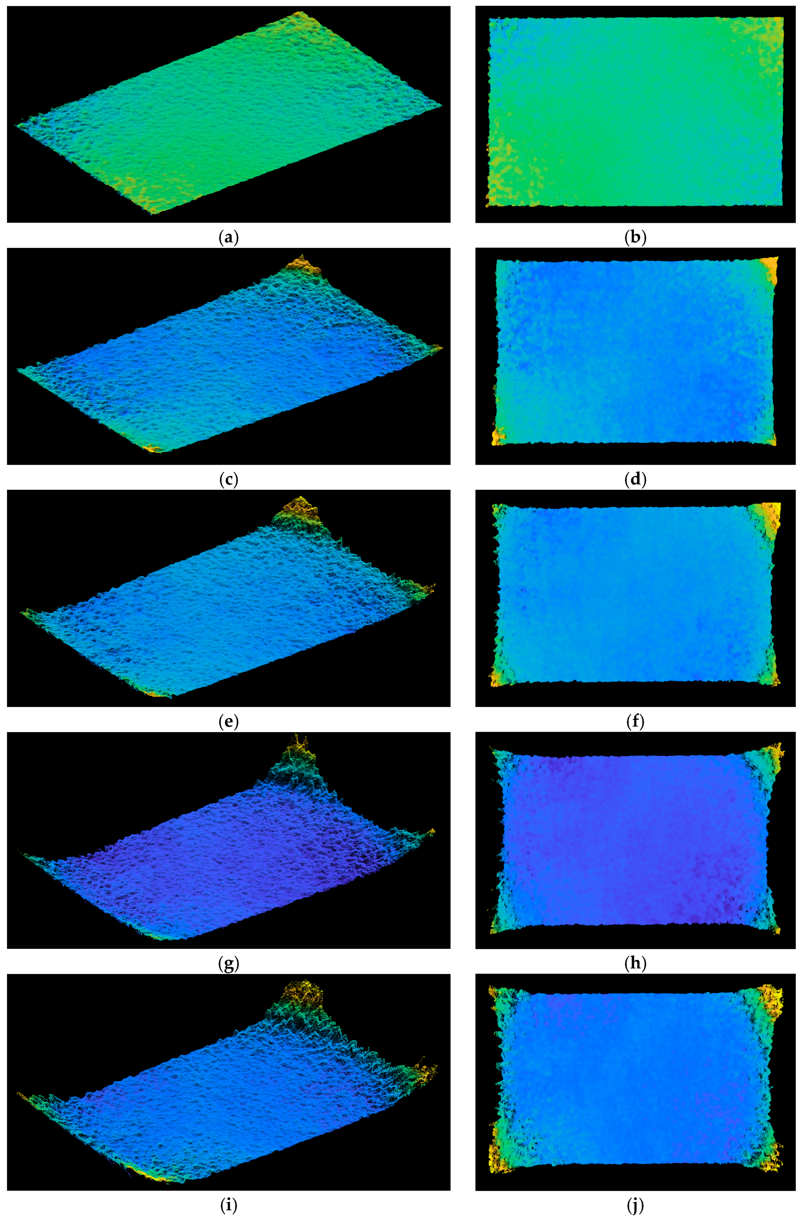
Figure 3 displays the original point cloud images of the five test datasets, revealing that the distortion around the edges becomes increasingly severe as the distance from the structured light LiDAR increases. Specifically, the contour edge of the object in the point clouds exhibit increasing distortion, highlighting the challenges of maintaining data accuracy in areas far from the sensor.
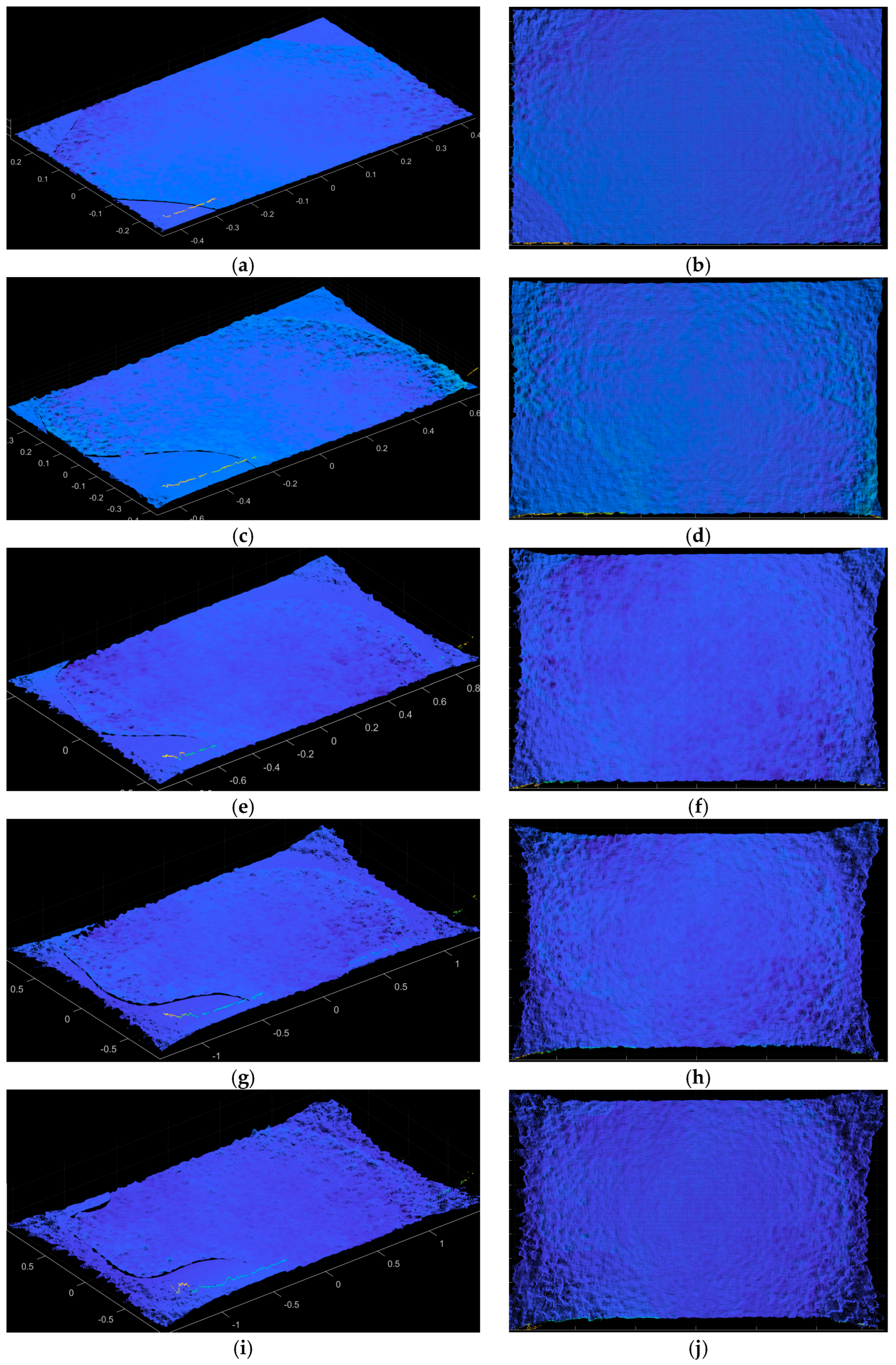
Figure 4 shows the point cloud images of five test datasets corrected by the 3D point cloud least mean square filter based on SVM. Through observation, it can be found that the SVM model only draws two boundaries between the signal region and the distorted region, which is rough and fails to accurately distinguish each point, meaning it cannot identify which points are signal points and which ones are distortion points.
Figure 5 shows the point cloud images of five test datasets corrected by the proposed D−LMS filtering algorithm. Under the guidance of the decision tree model for partitioning, the signal regions and distorted regions are intricately interleaved, allowing for precise identification of all distorted point clouds. Subsequently, these distorted point clouds can be accurately corrected using the adaptive least mean squares filter, ultimately yielding a high-precision point cloud image.
Table 3 summarizes the accuracy of different methods under five testing datasets. In this context, accuracy is defined as the ratio of the number of correct points to the total number of points. It takes into account both the original signal points that were accurately retained and the distorted points that were successfully corrected to their true positions. This provides a comprehensive measure of how well each method performs in terms of accuracy.
The experimental result shows that the D−LMS filtering algorithm can effectively improve the accuracy of point cloud images under five testing datasets, which demonstrates the superiority of the D−LMS filtering algorithm in terms of its ability to accurately correct point cloud data. Compared with the original point cloud image without algorithm processing, the accuracy of the proposed D−LMS filtering algorithm is improved from 72.69% to 92.38%. Compared with the 3D point cloud least square filter based on SVM, the accuracy of the proposed D−LMS filtering algorithm is improved from 86.17 to 92.38%. These results emphasize the effectiveness and efficiency of D−LMS filtering algorithm, which indicates that it can be widely used in the field of distortion calibration of 3D point cloud images.

5. Conclusions

In summary, this paper proposes a high-performance 3D point cloud Least Mean Square filter based on Decision Tree, which can address the challenges of distortion in point cloud images captured by Structured Light LiDAR. The proposed D−LMS filtering algorithm can effectively address the problems of lens scattering and temperature fluctuation, which are the primary factors causing distortion in the collected data. By utilizing the classification and prediction capabilities of the decision tree model, the D−LMS filtering algorithm can accurately differentiate between signal regions and distortion regions, and can automatically adjust its filtering parameters through the adaptive least mean square filter to accurately correct the distortion point. Compared with the original point cloud image, the D−LMS filter has significantly improved the accuracy of the point cloud image from 72.69% to 92.38%, which represents a significant advancement in the field of 3D point cloud image distortion calibration. Its high performance, adaptability and robustness make it a promising solution to improve the accuracy of point cloud data obtained by structured light lidar system.

Funding

This research received no external funding, and the article processing charge (APC) was funded by Yao Duan, the corresponding author of this article.

Institutional Review Board Statement

The study did not require ethical approval.

Informed Consent Statement

Not applicable.

Data Availability Statement

The datasets generated or analyzed during this study are not publicly available due to commercial confidentiality and proprietary restrictions. However, they may be obtained from the corresponding author upon reasonable request.

Conflicts of Interest

The authors declare that there are no conflicts of interest related to this article.

References

  1. Tu, D.; Cui, H.; Shen, S. PanoVLM: Low-Cost and accurate panoramic vision and LiDAR fused mapping. ISPRS J. Photogramm. Remote Sens. 2023, 206, 149–167. [Google Scholar] [CrossRef]
  2. Tachella, J.; Altmann, Y.; Mellado, N.; McCarthy, A.; Tobin, R.; Buller, G.S.; Tourneret, J.-Y.; McLaughlin, S. Real-time 3D reconstruction from single-photon lidar data using plug-and-play point cloud denoisers. Nat. Commun. 2019, 10, 4984. [Google Scholar] [CrossRef]
  3. Vines, P.; Kuzmenko, K.; Kirdoda, J.; Dumas, D.C.S.; Mirza, M.M.; Millar, R.W.; Paul, D.J.; Buller, G.S. High performance planar germanium-on-silicon single-photon avalanche diode detectors. Nat. Commun. 2019, 10, 1086. [Google Scholar] [CrossRef]
  4. Le Gentil, C.; Vidal-Calleja, T.; Huang, S. 3D Lidar-IMU Calibration Based on Upsampled Preintegrated Measurements for Motion Distortion Correction. In Proceedings of the 2018 IEEE International Conference on Robotics and Automation (ICRA), Brisbane, Australia, 21–25 May 2018; pp. 2149–2155. [Google Scholar]
  5. Han, Y.; Salido-Monzú, D.; Butt, J.A.; Schweizer, S.; Wieser, A. A feature selection method for multimodal multispectral LiDAR sensing. ISPRS J. Photogramm. Remote Sens. 2024, 212, 42–57. [Google Scholar] [CrossRef]
  6. Zhang, Y.; Li, S.; Sun, J.; Zhang, X.; Zhou, X.; Zhang, H. Noise-tolerant depth image estimation for array Gm-APD LiDAR through atmospheric obscurants. Opt. Laser Technol. 2024, 175, 110706. [Google Scholar] [CrossRef]
  7. Wu, M.; Lu, Y.; Li, H.; Mao, T.; Guan, Y.; Zhang, L.; He, W.; Wu, P.; Chen, Q. Intensity-guided depth image estimation in long-range lidar. Opt. Lasers Eng. 2022, 155, 107054. [Google Scholar] [CrossRef]
  8. Ni, H.; Sun, J.; Ma, L.; Liu, D.; Zhang, H.; Zhou, S. Research on 3D image reconstruction of sparse power lines by array GM-APD lidar. Opt. Laser Technol. 2024, 168, 109987. [Google Scholar] [CrossRef]
  9. Peng, Z.; Wang, H.; She, X.; Xue, R.; Kong, W.; Huang, G. Marine remote target signal extraction based on 128 line-array single photon LiDAR. Infrared Phys. Technol. 2024, 143, 105592. [Google Scholar] [CrossRef]
  10. Chen, M.; Rao, P.R.; Venialgo, E. Depth estimation in SPAD-based LiDAR sensors. Opt. Express 2024, 32, 3006–3030. [Google Scholar] [CrossRef] [PubMed]
  11. Gottfried, J.M.; Fehr, J.; Garbe, C.S. Computing Range Flow from Multi-Modal Kinect Data. In Proceedings of the Advances in Visual Computing: 7th International Symposium, ISVC 2011, Las Vegas, NV, USA, 26–28 September 2011; Part I 7. Springer: Berlin/Heidelberg, Germany, 2011; pp. 758–767. [Google Scholar]
  12. Zhang, Z. Microsoft kinect sensor and its effect. IEEE Multimed. 2012, 19, 4–10. [Google Scholar] [CrossRef]
  13. Han, J.; Shao, L.; Xu, D.; Shotton, J. Enhanced computer vision with microsoft kinect sensor: A review. IEEE Trans. Cybern. 2013, 43, 1318–1334. [Google Scholar] [CrossRef]
  14. Diego-Mas, J.A.; Alcaide-Marzal, J. Using Kinect™ sensor in observational methods for assessing postures at work. Appl. Ergon. 2014, 45, 976–985. [Google Scholar] [CrossRef]
  15. DiFilippo, N.M.; Jouaneh, M.K. Characterization of different Microsoft Kinect sensor models. IEEE Sens. J. 2015, 15, 4554–4564. [Google Scholar] [CrossRef]
  16. Khoshelham, K.; Elberink, S.O. Accuracy and resolution of Kinect depth data for indoor mapping applications. Sensors 2012, 12, 1437–1454. [Google Scholar] [CrossRef] [PubMed]
  17. Bähler, N.; El Helou, M.; Objois, É.; Okumuş, K.; Süsstrunk, S. Pogain: Poisson–Gaussian image noise modeling from paired samples. IEEE Signal Process. Lett. 2022, 29, 2602–2606. [Google Scholar] [CrossRef]
  18. Mannam, V.; Zhang, Y.; Zhu, Y.; Nichols, E.; Wang, Q.; Sundaresan, V.; Zhang, S.; Smith, C.; Bohn, P.W.; Howard, S.S. Real-time image denoising of mixed Poisson–Gaussian noise in fluorescence microscopy images using Image. Optica 2022, 9, 335–345. [Google Scholar] [CrossRef]
  19. Bahador, F.; Gholami, P.; Lakestani, M. Mixed Poisson–Gaussian noise reduction using a time–space fractional differential equations. Inf. Sci. 2023, 647, 119417. [Google Scholar] [CrossRef]
  20. Rusinkiewicz, S.; Levoy, M. Efficient variants of the ICP algorithm. In Proceedings of the Third International Conference on 3-D Digital Imaging and Modeling, Quebec City, QC, Canada, 28 May–1 June 2001; IEEE: Piscataway, NJ, USA, 2001; pp. 145–152. [Google Scholar]
  21. Chen, H.-X.; Li, K.; Fu, Z.; Liu, M.; Chen, Z.; Guo, Y. Distortion-aware monocular depth estimation for omnidirectional images. IEEE Signal Process. Lett. 2021, 28, 334–338. [Google Scholar] [CrossRef]
  22. Narawade, N.S.; Kanphade, R.D. Geometric distortion correction in images using proposed spy pixel and size. In Proceedings of the 2014 International Conference on Advances in Computing, Communications and Informatics (ICACCI), Delhi, India, 24–27 September 2014; IEEE: Piscataway, NJ, USA, 2014; pp. 1413–1417. [Google Scholar]
  23. Yothers, M.P.; Browder, A.E.; Bumm, L.A. Real-space post-processing correction of thermal drift and piezoelectric actuator nonlinearities in scanning tunneling microscope images. Rev. Sci. Instrum. 2017, 88, 013705. [Google Scholar] [CrossRef]
  24. Wu, Y.; Fan, Z.; Fang, Y.; Liu, C. An effective correction method for AFM image distortion due to hysteresis and thermal drift. IEEE Trans. Instrum. Meas. 2020, 70, 1–12. [Google Scholar] [CrossRef]
  25. Van de Weijer, J.; Van den Boomgaard, R. Local mode filtering. In Proceedings of the 2001 IEEE Computer Society Conference on Computer Vision and Pattern Recognition, CVPR 2001, Kauai, HI, USA, 8–14 December 2001; IEEE: Piscataway, NJ, USA, 2001; Volume 2, p. II-II. [Google Scholar]
  26. He, K.; Sun, J.; Tang, X. Guided image filtering. IEEE Trans. Pattern Anal. Mach. Intell. 2012, 35, 1397–1409. [Google Scholar] [CrossRef]
  27. Liu, S.; Lai, P.; Tian, D.; Gomila, C.; Chen, C.W. Joint trilateral filtering for depth map compression. In Proceedings of the Visual Communications and Image Processing 2010, Huangshan, China, 11–14 July 2010; SPIE: Bellingham, WA, USA, 2010; Volume 7744, pp. 132–141. [Google Scholar]
  28. Oh, K.J.; Vetro, A.; Ho, Y.S. Depth coding using a boundary reconstruction filter for 3-D video systems. IEEE Trans. Circuits Syst. Video Technol. 2011, 21, 350–359. [Google Scholar] [CrossRef]
  29. Xu, X.; Po, L.M.; Cheung, T.C.H.; Cheung, K.W.; Feng, L.; Ting, C.W.; Ng, K.H. Adaptive depth truncation filter for MVC-based compressed depth image. Signal Process. Image Commun. 2014, 29, 316–331. [Google Scholar] [CrossRef]
  30. Zhao, L.; Wang, A.; Zeng, B.; Wu, Y. Candidate value-based boundary filtering for compressed depth images. Electron. Lett. 2015, 51, 224–226. [Google Scholar] [CrossRef]
  31. Zhao, L.; Bai, H.; Wang, A.; Zhao, Y.; Zeng, B. Two-stage filtering of compressed depth images with Markov random field. Signal Process. Image Commun. 2017, 54, 11–22. [Google Scholar] [CrossRef]
  32. Charbuty, B.; Abdulazeez, A. Classification based on decision tree algorithm for machine learning. J. Appl. Sci. Technol. Trends 2021, 2, 20–28. [Google Scholar] [CrossRef]
  33. Karchi, N.; Kulkarni, D.; Pérez de Prado, R.; Divakarachari, P.B.; Patil, S.N.; Desai, V. Adaptive least mean square controller for power quality enhancement in solar photovoltaic system. Energies 2022, 15, 8909. [Google Scholar] [CrossRef]
  34. Nagabushanam, M.; Chakrasali, S.; Gangadharaiah, S.L.; Patel, S.H.; Ramaiah, G.; Basak, R. An Optimized VLSI Implementation of the Least Mean Square (LMS) Adaptive Filter Architecture on the Basis of Distributed Arithmetic Approach. J. Inst. Eng. India Ser. B 2024, 106, 861–870. [Google Scholar] [CrossRef]
  35. Rosalin; Rout, N.K.; Das, D.P. Adaptive Exponential Trigonometric Functional Link Neural Network Based Filter Proportionate Maximum Versoria Least Mean Square Algorithm. J. Vib. Eng. Technol. 2024, 12, 8829–8837. [Google Scholar] [CrossRef]
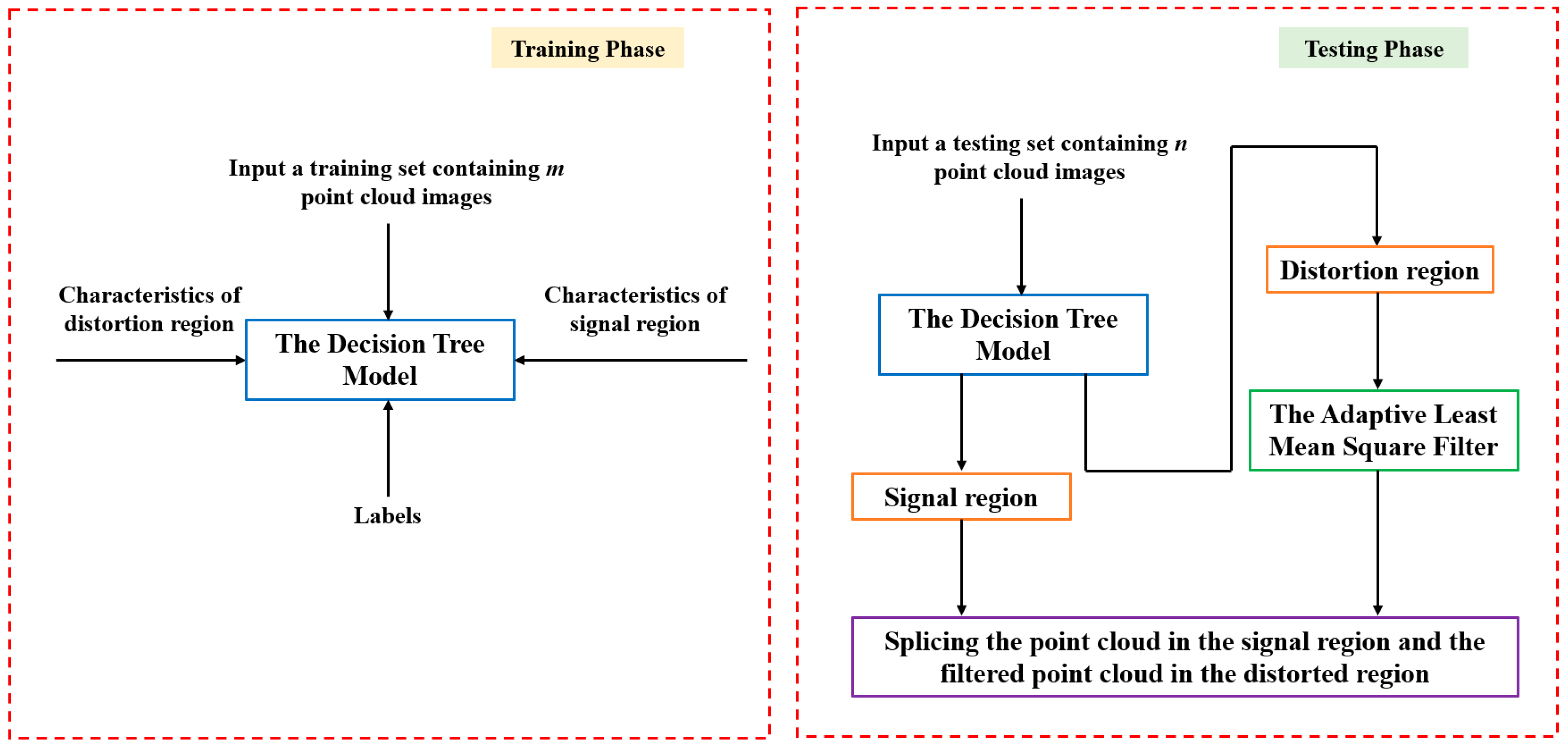
Figure 1. The outline of the proposed D−LMS filter.
Photonics 12 00960 g001
Figure 2. An overview of some training datasets.
Photonics 12 00960 g002
Figure 3. The original point cloud images of the five test datasets: (a,b) are the full view and front view of dataset 1, (c,d) are the full view and front view of dataset 2, (e,f) are the full view and front view of dataset 3, (g,h) are the full view and front view of dataset 4, and (i,j) are the full view and front view of dataset 5.
Photonics 12 00960 g003
Figure 4. The point cloud images of five test datasets corrected by the 3D point cloud least mean square filter based on SVM: (a,b) are the full view and front view of dataset 1, (c,d) are the full view and front view of dataset 2, (e,f) are the full view and front view of dataset 3, (g,h) are the full view and front view of dataset 4, and (i,j) are the full view and front view of dataset 5.
Photonics 12 00960 g004
Figure 5. The point cloud images of five test datasets corrected by the proposed D−LMS filtering algorithm: (a,b) are the full view and front view of dataset 1, (c,d) are the full view and front view of dataset 2, (e,f) are the full view and front view of dataset 3, (g,h) are the full view and front view of dataset 4, and (i,j) are the full view and front view of dataset 5.
Photonics 12 00960 g005
Table 1. Complexity Analysis of Different Methods.
AlgorithmTraining TimeTesting Time
3D point cloud least mean square filter based on SVM1726.25 s72.52 s
The proposed D−LMS filtering algorithm1.31 s0.06 s
Table 2. The number of points in the signal region and the distortion region for different test datasets.
The Testing DatasetDistanceNumber of Points in Signal RegionNumber of Points in Distorted Region
Dataset 10.6 m231,6519646
Dataset 20.9 m211,05129,800
Dataset 31.2 m199,53641,316
Dataset 41.6 m175,47364,782
Dataset 51.9 m172,82964,940
Table 3. The accuracy of different methods under five testing datasets.
AlgorithmDataset 1Dataset 2Dataset 3Dataset 4Dataset 5
Without algorithm processing96.00%87.63%82.85%73.04%72.69%
3D point cloud least mean square filter based on SVM98.87%95.78%92.39%87.54%86.17%
The proposed D−LMS filtering algorithm99.52%97.25%95.03%93.55%92.38%
Disclaimer/Publisher’s Note: The statements, opinions and data contained in all publications are solely those of the individual author(s) and contributor(s) and not of MDPI and/or the editor(s). MDPI and/or the editor(s) disclaim responsibility for any injury to people or property resulting from any ideas, methods, instructions or products referred to in the content.